A central limit theorem for scaled eigenvectors of random dot product graphs

Abstract

We prove a central limit theorem for the components of the largest eigenvectors of the adjacency matrix of a finite-dimensional random dot product graph whose true latent positions are unknown. In particular, we follow the methodology outlined in Sussman et al. (2014) to construct consistent estimates for the latent positions, and we show that the appropriately scaled differences between the estimated and true latent positions converge to a mixture of Gaussian random variables. As a corollary, we obtain a central limit theorem for the first eigenvector of the adjacency matrix of an Erdös-Renyi random graph.

1 Introduction

Spectral analysis of the adjacency and Laplacian matrices for graphs is of both theoretical (Chung, 1997) and practical (Luxburg, 2007) significance. For instance, the spectrum can be used to characterize the number of connected components in a graph and various properties of random walks on graphs, and the eigenvector corresponding to the second smallest eigenvalue of the Laplacian is used in the solution to a relaxed version of the min-cut problem (Fiedler, 1973). In our current work, we investigate the second-order properties of the eigenvectors corresponding to the largest eigenvalues of the adjacency matrix of a random graph. In particular, we show that under the random dot product graph model (Young and Scheinerman, 2007), the components of the eigenvectors are asymptotically normal and centered around the true latent positions (see Section 4). We consider only undirected, loop-free graphs in which the expected number of edges grows as $\Theta(n^{2})$. However, the results contained here can be extended to sparse graphs.

This paper is organized as follows: in Section 2 we provide background and give a brief overview of related work. In Section 3 we prove a central limit theorem for the difference between the estimated and true latent positions for the one-dimensional random dot product graph. We present the proof of the one-dimensional case first because it illustrates, in a simpler setting, the main ideas of the proof in higher dimensions. We then note two corollaries for special cases of random dot product graphs. In Section 4 we derive the central limit theorem for multi-dimensional random dot product graphs, and in Section 5 we demonstrate our results via simulation. Finally we conclude the paper in Section 6 with further discussion.

2 Background and Related Work

This work is concerned with the eigenvectors corresponding to the largest eigenvalues of the adjacency matrix of a random dot product graph. Random dot product graphs are a specific example of latent position random graphs (Hoff et al., 2002), in which each vertex is associated with a latent position and, conditioned on the latent positions, the presence or absence of all edges in the graph are independent. The edge presence probability is based on link function, which is a symmetric function of the two latent positions.

We note briefly that, in a strong sense, latent position graphs are identical to exchangeable random graphs (Aldous, 1981; Hoover, 1979), with the key unifying ingredient being the conditional independence of the edges. A fundamental result on exchangeable graphs is the notion of a graph limit which is constructed via subgraph counts (Diaconis and Janson, 2008). The work of Diaconis and Janson has important consequences in statistical inference, for instance the method of moments for subgraph counts (Bickel et al., 2011). In a similar spirit, our current results provide asymptotic distributions for spectral statistics that have the promise to improve current statistical methodology for random graphs (see § 5).

Statistical analysis for latent position random graphs has received much recent interest: see Goldenberg et al. (2010) and Fortunato (2010) for reviews of the pertinent literature. Some fundamental results are found in Bickel et al. (2011); Bickel and Chen (2009); Choi et al. (2012) among many others. In the statistical analysis of latent position random graphs, a common strategy is to first estimate the latent positions based on some specified link function. For example, in random dot product graphs (Young and Scheinerman, 2007), the link function is the dot product: namely, the edge probabilities are the dot products of the latent positions. Sussman et al. (2014) show that spectral decompositions of the adjacency matrix for a random dot product graphs provide accurate estimates of the underlying latent positions. In this work, we extend the analysis in Sussman et al. (2014) to show a distributional convergence of the residuals between the estimated and true latent positions.

Our work is also influenced by the analysis of the spectra of random graphs (Chung, 1997). Of special note is the classic paper of Füredi and Komlós (1981), in which the authors show that for an Erdös-Rényi graph with parameter $p$, the appropriately scaled largest eigenvalue of the adjacency matrix converges in law to a normal distribution. Other results of this type are proved for sparse graphs in both the independent edge model (Krivelevich and Sudakov, 2003) and the $d$-regular random graph model (Janson, 2005). More recently, general bounds for the operator norm of the difference between the adjacency matrix and its expectation have been proved in Oliveira (2010) and Tropp (2011) (see Proposition 3.2, Eq. (3.5)).

We would, of course, be remiss not to mention important recent results in random matrix theory. In particular, a recent result by Tao and Vu (2012) proves a central limit theorem for the eigenvectors of a mean zero random symmetric matrix with independent entries. Tao and Vu (2012) prove a result for eigenvectors corresponding to the bulk of the spectra and Knowles and Yin (2011) prove a similar result for eigenvectors near the “edge” of the spectra. A material difference between these results and our present work, however, is that we consider random matrices whose entries have nonzero mean. For mean zero matrices, the eigenvalues and eigenvectors that are most readily studied are not the largest in magnitude but those in the “bulk” of the spectra, while in our setting, the structure of the mean matrix eases the study of the largest eigenvalues and their corresponding eigenvectors.

As will be seen in Section 3, the key step in our work is to apply the power method to the adjacency matrix, with the initial vector the true latent position. Conditioned on the true latent position, this produces a vector whose components are asymptotically normally distributed. Furthermore, the difference between this vector and the true eigenvector of the adjacency matrix is asymptotically negligible, due to a large gap between the largest eigenvalue and the remaining eigenvalues.

Finally, we note that a recent paper of Yan and Xu (2013) which provides a proof of the asymptotic normality for maximum likelihood estimates of the parameters of a related model, i.e. the logistic $\beta$-model, and derived the associated Fisher information matrix. The $\beta$-model also belongs to the class of latent position models. It is thus of potential interests to derive the Fisher information for the random dot product graph model as considered in this work.

3 Central limit theorem for one-dimensional random dot product graphs

In this section, we state and prove a central limit theorem for a one-dimensional random dot product graph, defined as follows.

Definition 3.1 (Random Dot Product Graph ($d$=1)).

For a distribution $F$ on $[0,1]$, we say that $(X,A)\sim\mathrm{RDPG}(F)$ if the following hold. Let $X_{1},\dotsc,X_{n}{\sim}F$ be independent random variables and define

$$X=[X_{1},\dotsc,X_{n}]^{\top}\in\mathbb{R}^{n\times 1}\text{ and }P=XX^{\top}\in[0,1]^{n\times n}.$$ (3.1)

The $X_{i}$’s are the latent positions for the random graph with adjacency matrix $A$, where $A\in\{0,1\}^{n\times n}$ is defined to be a symmetric, hollow matrix such that for all $i<j$, conditioned on $X_{i}$ and $X_{j}$,

$$A_{ij}\stackrel{{\scriptstyle ind}}{{\sim}}\mathrm{Bern}(X_{i}X_{j}).$$ (3.2)

We remark that this one-dimensional model is a slight modification of the rank 1 inhomogeneous random graph model studied as an example in Bollobás et al. (2007).

Given $A$, it is often important to estimate $X$. Our estimate for $X$, which we denote $\widehat{X}$, is defined by $\widehat{X}=\widehat{\lambda}^{1/2}\widehat{V}$, where $\widehat{\lambda}=\lambda_{1}(A)$ is the largest eigenvalue of $A$ and $\widehat{V}$ its associated eigenvector, normalized to be of unit length. We define $V=X/\|X\|$, so $V$ is the normalized true latent positions. Let $\delta=\mathbb{E}[X_{1}^{2}]$ be the second moment of the latent positions.

Throughout this work, we will need explicit control on the differences, in Frobenius norm, between $X$ and $\widehat{X}$ and $V$ and $\widehat{V}$. We state here the necessary bounds in the one-dimensional case. These bounds are special cases of the more general bounds in the finite-dimensional setting of § 4. The proofs for the finite-dimensional bounds are given in Sussman et al. (2014) and Oliveira (2010).

Proposition 3.2.

Let $\delta=\mathbb{E}[X_{1}^{2}]$, $V=X/\|X\|$ and $\widehat{V}=\widehat{X}/\|\widehat{X}\|$. Let $c>0$ be arbitrary. There exists a constant $n_{0}(c)$ such that if $n>n_{0}$, then for any $\eta$ satisfying $n^{-c}<\eta<1/2$, the following bounds hold with probability greater than $1-\eta$,

$$\|X-\widehat{X}\| \leq 4\delta^{-1}\sqrt{2\log(n/\eta)},$$ (3.3)

$$\|V-\widehat{V}\| \leq 4\delta^{-1}\sqrt{\frac{\log(n/\eta)}{n}},$$ (3.4)

$$\text{ and }\|XX^{\top}-A\| \leq 2\sqrt{n\log{(n/\eta)}}.$$ (3.5)

Hence, the above bounds imply that for $n$ sufficiently large, with probability greater than $1-\eta$,

$$\frac{\delta n}{2}\leq\|P\|\leq n,\quad\frac{\delta n}{2}\leq\|A\|\leq n.$$ (3.6)

where $\|\cdot\|$ represents the spectral norm for matrices and the $\ell_{2}$ vector norm for vectors.

We emphasize that a number of our subsequent arguments focus on events that occur with probability at least $1-\eta$; it is assumed that $c$ is suitably chosen and $n$ is sufficiently large to ensure that $n^{-c}\leq\eta\leq 1/2$.

Our aim in this section is to prove the following limit theorem.

Theorem 3.3.

Let $(X,A)\sim\mathrm{RDPG}(F)$ and let $\widehat{X}$ be our estimate for $X$. Let $\Phi(z,\sigma^{2})$ denote the normal cumulative distribution function, with mean zero and variance $\sigma^{2}$, evaluated at $z$. Then for each component $i$ and any $z\in\mathbb{R}$,

$$\mathbb{P}\Bigl{\{}\sqrt{n}\bigl{(}\widehat{X}_{i}-X_{i}\bigr{)}\leq z\Bigr{\}}\rightarrow\int\Phi(z,\delta^{-2}\sigma^{2}(x_{i}))dF(x_{i})$$

where $\sigma^{2}(x_{i})=x_{i}\mathbb{E}[X_{1}^{3}]-x_{i}^{2}\mathbb{E}[X_{1}^{4}]$ and $\delta=\mathbb{E}[X_{1}^{2}].$ That is, the sequence of random variables $\sqrt{n}(\widehat{X}_{i}-X_{i})$ converges in distribution to a mixture of normals. We denote this mixture by $\mathcal{N}(0,\delta^{-2}\sigma^{2}(X_{i}))$.

As an immediate consequence, we obtain the following corollary for the eigenvectors of an Erdös-Rényi random graph. For the Erdös-Renyi graph, the $X_{i}$ have a degenerate distribution; namely, there is some $p\in(0,1)$ such that $X_{i}=\sqrt{p}$ for all $i$.

Corollary 3.4.

For an Erdös-Renyi ($p$) graph, the following central limit theorem holds:

$$\sqrt{n}(\widehat{X}_{i}-\sqrt{p})\stackrel{{\scriptstyle\mathcal{L}}}{{\longrightarrow}}\mathcal{N}(0,1-p).$$

To prove Theorem 3.3, we will need Proposition 3.2 and a succession of simpler lemmas. To begin, we apply one step of the power method, with initial vector $V$. In particular, let $Y=\widehat{\lambda}^{-1/2}AV$ be the vector in $\mathbb{R}^{n}$ with components $Y_{i}=\widehat{\lambda}^{-1/2}\sum_{j=1}^{n}A_{ij}V_{j}$.

Proposition 3.5.

Taking $X_{i}=x_{i}$ as given, we have

$$\sqrt{n}\Bigl{(}Y_{i}-\frac{\|X\|}{\widehat{\lambda}^{1/2}}x_{i}\Bigr{)}\stackrel{{\scriptstyle\mathcal{L}}}{{\longrightarrow}}\mathcal{N}(0,\delta^{-2}\sigma^{2}(x_{i}))$$

where $\sigma^{2}(\cdot)$ and $\delta$ are as in Theorem 3.3.

Proof.

Observe that

$$\sqrt{n}\Bigl{(}Y_{i}-\frac{\|X\|}{\widehat{\lambda}^{1/2}}x_{i}\Bigr{)} =\frac{\sqrt{n}}{\widehat{\lambda}^{1/2}}\Bigl{(}\sum_{j=1}^{n}A_{ij}V_{j}-\|X\|x_{i}\Bigr{)}$$

$$=\frac{\sqrt{n}}{\widehat{\lambda}^{1/2}\|X\|}\Bigl{(}\sum_{j=1}^{n}A_{ij}X_{j}-x_{i}\|X\|^{2}\Bigr{)}$$

$$=\frac{n}{\widehat{\lambda}^{1/2}\|X\|}\ast\frac{1}{\sqrt{n}}\Bigl{[}\Bigl{(}\sum_{j\neq i}(A_{ij}-x_{i}X_{j})X_{j}\Bigr{)}-x_{i}^{3}\Bigr{]}$$

The scaled sum

$$\frac{1}{\sqrt{n}}\Bigl{(}\sum_{j\neq i}(A_{ij}-x_{i}X_{j})X_{j}\Bigr{)}$$

is a sum of independent, identically distributed random variables each with mean zero and variance

$$\sigma^{2}(x_{i})=x_{i}\mathbb{E}[X_{j}^{3}]-x_{i}^{2}\mathbb{E}[X_{j}^{4}].$$

The classical Lindeberg-Feller central limit theorem and Slutsky’s Theorem (Chung, 2001, Theorem 7.2.1 and Theorem 4.4.6) imply that

$$\frac{1}{\sqrt{n}}\Bigl{[}\Bigl{(}\sum_{j\neq i}(A_{ij}-x_{i}X_{j})X_{j}\Bigr{)}-x_{i}^{3}\Bigr{]}\stackrel{{\scriptstyle\mathcal{L}}}{{\longrightarrow}}\mathcal{N}(0,\sigma^{2}(x_{i})).$$ (3.7)

Furthermore, the Strong Law implies that $\|X\|^{2}/n\rightarrow\delta$, and (3.5) and (3.6) in Proposition 3.2, along with the Borel-Cantelli Lemma, imply that $n/(\widehat{\lambda}^{1/2}\|X\|)$ converges almost surely to $\delta^{-1}$. Finally, another application of Slutsky’s Theorem allows us to conclude that

$$\sqrt{n}\Bigl{(}Y_{i}-\frac{\|X\|}{\widehat{\lambda}^{1/2}}x_{i}\Bigr{)}\stackrel{{\scriptstyle\mathcal{L}}}{{\longrightarrow}}\mathcal{N}(0,\delta^{-2}\sigma^{2}(x_{i}))$$

as desired. ∎

We remark that Proposition 3.2 and the Borel-Cantelli Lemma imply that $n/(\widehat{\lambda}^{1/2}\|X\|)\rightarrow\delta^{-1}$ with probability one, but we will need additional control of the rate of this convergence. We use the notation $Y_{n}=O_{\mathbb{P}}(\alpha(n))$ to denote that the sequence of random variables $Y_{n}/\alpha(n)$ is bounded in probability; and $Y_{n}=o_{\mathbb{P}}(\alpha(n))$ to denote that the sequence of random variables $Y_{n}/\alpha(n)$ converges to zero in probability. The next lemma shows that the factor $(1-\|X\|/\widehat{\lambda}^{1/2})=o_{\mathbb{P}}(1/\sqrt{n})$ . As a remark, for ease of exposition, some of the subsequent results and proofs in this paper, e.g., Proposition 3.8, will contain bounds with universal but hidden constants that do not depend on the parameters—that is, they do not depend on $n$, $\eta$ or $\delta$. We use the convention that these hidden constants are all denoted by a generic symbol $C$ and can change from line to line in the paper.

Lemma 3.6.

In the setting of Theorem 3.3, $\sqrt{n}\Bigl{(}1-\widehat{\lambda}^{-1/2}\|X\|\Bigr{)}\stackrel{{\scriptstyle p}}{{\longrightarrow}}0$.

Proof.

First, we have

$$1-\frac{\|X\|}{\widehat{\lambda}^{1/2}}=\frac{\widehat{\lambda}-\|X\|^{2}}{\widehat{\lambda}^{1/2}(\|X\|+\widehat{\lambda}^{1/2})}.$$ (3.8)

By Proposition 3.2, the denominator of Eq. (3.8) is bounded by

$$\widehat{\lambda}^{1/2}(\|X\|+\widehat{\lambda}^{1/2})\geq\frac{\delta n}{2}$$

with probability at least $1-\eta$. Since

$$\|X\|^{2}=\lambda_{1}(P)=V^{\top}PV\textrm{ and }\widehat{\lambda}=\widehat{V}^{\top}A\widehat{V},$$

it follows that

$$\Bigl{|}\|X\|^{2}-\widehat{\lambda}\Bigr{|}\leq|V^{\top}PV-V^{\top}AV|+|V^{\top}AV-\widehat{V}^{\top}A\widehat{V}|.$$ (3.9)

For the second term on the right-hand-side of (3.9), first observe that

$$|V^{\top}AV-\widehat{V}^{\top}A\widehat{V}| =|(V-\widehat{V})^{\top}A(V-\widehat{V})+2(V-\widehat{V})^{\top}A\widehat{V}|$$

$$=|(V-\widehat{V})^{\top}A(V-\widehat{V})+2\widehat{\lambda}(V-\widehat{V})^{\top}\widehat{V}|$$

$$\leq|(V-\widehat{V})^{\top}A(V-\widehat{V})|+|2\widehat{\lambda}(V-\widehat{V})^{\top}\widehat{V}|$$

$$\leq\widehat{\lambda}\|V-\widehat{V}\|^{2}+2\widehat{\lambda}|(V-\widehat{V})^{\top}\widehat{V}|$$

Now observe that

$$|\widehat{V}^{\top}(V-\widehat{V})|=\frac{1}{2}|\widehat{V}^{\top}V-\widehat{V}^{\top}\widehat{V}+V^{\top}\widehat{V}-V^{\top}V|=\frac{1}{2}\|V-\widehat{V}\|^{2}$$ (3.10)

and this implies that with probability at least $1-\eta$,

$$|V^{\top}AV-\widehat{V}^{\top}A\widehat{V}|\leq 2\widehat{\lambda}\|V-\widehat{V}\|^{2}\leq\frac{C\log(n/\eta)}{\delta^{2}},$$ (3.11)

for some constant $C$, by Proposition 3.2. For the first term in Eq. 3.9, we have

$$\begin{split}|V^{\top}AV-V^{\top}PV|&=|\sum_{i,j}(A_{ij}-P_{ij})V_{i}V_{j}|\\ &\leq|2\sum_{i<j}(A_{ij}-P_{ij})V_{i}V_{j}+\sum_{i}P_{ii}V_{i}^{2}|\\ &\leq|2\sum_{i<j}(A_{ij}-P_{ij})V_{i}V_{j}+\sum_{i}V_{i}^{2}|\\ &\leq|2\sum_{i<j}(A_{ij}-P_{ij})V_{i}V_{j}+1|\end{split}$$ (3.12)

The term $2\sum_{i<j}(A_{ij}-P_{ij})V_{i}V_{j}$ in Eq.(4.10) is the sum of $\binom{n}{2}$ independent random variables and we can use Hoeffding’s inequality to conclude that

$$\begin{split}\mathbb{P}[|\sum_{i<j}2(A_{ij}-P_{ij})V_{i}V_{j}|\geq t]&\leq 2\exp\Bigl{(}\frac{-2t^{2}}{\sum_{i<j}(2V_{i}V_{j})^{2}}\Bigr{)}\\ &\leq 2\exp\Bigl{(}\frac{-t^{2}}{\sum_{i=1}^{n}\sum_{j=1}^{n}(V_{i}V_{j})^{2}}\Bigr{)}\\ &\leq 2\exp(-t^{2}).\end{split}$$

where the last line follows from the fact that $V$ is a unit vector. Therefore, this bound is independent of the choice of $V$. Hence, the first term in Eq.(3.9) satisfies

$$\mathbb{P}[|V^{\top}(A-P)V|\leq C\sqrt{\log(1/\eta)}+1]\geq 1-\eta.$$

Putting together the bounds on the two terms in Eq. (3.9) yields the bound

$$|\|X\|^{2}-\widehat{\lambda}|\leq\frac{C\log{(n/\eta)}}{\delta^{2}}$$

with probabilty at least $1-\eta$. We therefore have $1-\widehat{\lambda}^{-1/2}\|X\|=O_{\mathbb{P}}(1/n)$ and the claim in Lemma 3.6 follows. ∎

Remark 3.7.

The proof of the previous lemma shows that with high probability, $|\widehat{\lambda}-\|X\|^{2}|\leq C\log n$ for some $C$ depending only on the distribution $F$. This bound is similar in kind to the central limit theorem, proved in Füredi and Komlós (1981), for the largest eigenvalue of an Erdös-Rényi random graph. Alon et al. (2002) also provide similar concentration rates for the first eigenvalue, namely that $|\lambda-\mathbb{E}[\lambda]|$ can be tightly controlled, which is somewhat different from our result. This result also greatly improves on the bound one obtains using only the operator norm bound of Oliveira (2010) (see Proposition 3.2).

Finally, we prove a bound on the $\ell_{2}$ distance between $\widehat{\lambda}^{-1/2}AV$ and $\widehat{X}$.

Proposition 3.8.

Let $Y=\widehat{\lambda}^{-1/2}AV$. Provided the events in Theorem  3.2 occur, we have

$$\|Y-\widehat{X}\|\leq\frac{C\log(n/\eta)}{\sqrt{n\delta^{3}}}.$$

Proof.

Let $E=A-P=A-XX^{\top}$. We have

$$\begin{split}\|Y-\widehat{X}\|&=\widehat{\lambda}^{-1/2}\|A(V-\widehat{V})\|\\ &=\widehat{\lambda}^{-1/2}\|(\widehat{\lambda}\widehat{V}\widehat{V}^{\top}+E)(V-\widehat{V})\|\\ &\leq\widehat{\lambda}^{1/2}|\widehat{V}^{\top}(V-\widehat{V})|+\widehat{\lambda}^{-1/2}\|E(V-\widehat{V})\|\end{split}$$

Using Eq. (3.10) and $\sqrt{\delta n}/2\leq\widehat{\lambda}^{1/2}\leq 2\sqrt{\delta n}$, the term $\widehat{\lambda}^{1/2}|\widehat{V}^{\top}(V-\widehat{V})|$ is bounded above by $C\delta^{-3/2}n^{-1/2}\log(n/\eta)$. By Proposition 3.2, $\|E\|\leq 2\sqrt{n\log(n/\eta)}$, and therefore

$$\begin{split}\widehat{\lambda}^{-1/2}\|E(V-\widehat{V})\|&\leq\widehat{\lambda}^{-1/2}\|E\|\ast\|(V-\widehat{V})\|\leq\frac{C\log{(n/\eta)}}{\sqrt{n\delta^{3}}}\end{split}$$

from which the desired bound follows. ∎

We are now equipped to prove our limit theorem:

Proof of Theorem 3.3.

Integrating over the possible realizations of $X_{i}$ in Proposition 3.5 and applying the dominated convergence theorem, we deduce that

$$\mathbb{P}\Bigl{\{}\sqrt{n}\Bigl{(}Y_{i}-\frac{\|X\|}{\widehat{\lambda}^{1/2}}X_{i}\Bigr{)}\leq z\Bigr{\}}\rightarrow\int\Phi(z,\delta^{-2}\sigma^{2}(x_{i}))dF(x_{i}).$$

This establishes that

$$\sqrt{n}\Bigl{(}Y_{i}-\frac{\|X\|}{\widehat{\lambda}^{1/2}}X_{i}\Bigr{)}\rightarrow\mathcal{N}(0,\delta^{-2}\sigma^{2}(X_{i})).$$

Markov’s inequality, the exchangeability of $\{Y_{i}-\widehat{X}_{i}\}_{i=1}^{n}$, and the bounds in Prop. 3.8 allow us to conclude that

$$\mathbb{P}[\sqrt{n}|Y_{i}-\widehat{X}_{i}|>\epsilon]\leq\frac{\mathbb{E}[n(Y_{i}-\widehat{X}_{i})^{2}]}{\epsilon^{2}}=\frac{\mathbb{E}[\|Y-\widehat{X}\|^{2}]}{\epsilon^{2}}\leq\frac{C\log^{2}{n}}{\epsilon^{2}n}.$$

for some constant $C$ that is independent of $n$ and $\epsilon$. Hence $\sqrt{n}(Y_{i}-\widehat{X}_{i})$ converges to zero in probability. Observe that

$$\sqrt{n}\Bigl{(}\widehat{X}_{i}-\frac{\|X\|}{\widehat{\lambda}^{1/2}}X_{i}\Bigr{)}=\sqrt{n}(\widehat{X}_{i}-Y_{i})+\sqrt{n}\Bigl{(}Y_{i}-\frac{\|X\|}{\widehat{\lambda}^{1/2}}X_{i}\Bigr{)},$$

and Theorem 3.3 follows from the convergence to zero in probability of the first summand, the convergence in distribution to a Gaussian mixture of the second summand, and Lemma 3.6. ∎

3.1 Corollaries

In this section, we prove three corollaries, each of which is either a special case or an extension of Theorem 3.3. First, we demonstrate that in the stochastic blockmodel, if we condition on $X_{i}=x$, the residuals converge to the correct mixture component; second, we prove a similar result in the case where the latent position distribution has a density and we condition on $X_{i}$ belonging to any set of positive $F$-measure, where $F$ is the distribution of the latent positions; and finally, we prove a central limit theorem for the distribution of any fixed number $k$ of the residuals, $\sqrt{n}(\widehat{X}_{i}-X_{i})$, for $1\leq i\leq k$. We begin with the first corollary, in which we obtain appropriate convergence to the correct mixture component for the stochastic blockmodel, as defined in the statement of Corollary 3.9 below.

Corollary 3.9.

In the setting of Theorem 3.3, let $\mathcal{X}=\mathrm{supp}(F)\subset[0,1]$ be the support of the distribution of the $X_{i}$ and suppose that $|\mathcal{X}|=m<\infty$. Suppose for each $x\in\mathcal{X}$, we have that $\mathbb{P}[X_{i}=x]=\pi_{x}>0$. Then for all $x\in\mathcal{X}$, if we condition on $X_{i}=x$, we obtain

$$\mathbb{P}\Bigl{\{}n^{1/2}(\widehat{X}_{i}-x)\leq z\mid X_{i}=x\Bigr{\}}{\longrightarrow}\Phi(z,\delta^{-2}\sigma^{2}(x))$$ (3.13)

where $\sigma^{2}(\cdot)$ and $\delta$ are as in Theorem 3.3.

Proof.

Let $p_{n}(x,\epsilon)=\mathbb{P}(n^{1/2}|\widehat{X_{i}}-Y_{i}|>\epsilon\mid X_{i}=x)$ where $Y=\widehat{\lambda}^{-1/2}AV$ is as in Proposition 3.8. By Proposition 3.5 and Slutsky’s Theorem, we need only show that for all $\epsilon>0$ and $x\in\mathcal{X}$,

$$p_{n}(x,\epsilon)\to 0\textrm{ as }n\to\infty,$$ (3.14)

because this yields

$$n^{1/2}\Bigl{(}\widehat{X}_{i}-\frac{\|X\|}{\widehat{\lambda}^{1/2}}x\Bigr{)}\stackrel{{\scriptstyle\mathcal{L}}}{{\longrightarrow}}\mathcal{N}(0,\delta^{-2}\sigma^{2}(x)).$$ (3.15)

First, by Markov’s inequality, Proposition 3.8 , and the exchangeability of the sequence $\widehat{X}_{i}-Y_{i}$, we have

$$\mathbb{P}\Bigl{(}n^{1/2}|\widehat{X_{i}}-Y_{i}|>\epsilon\Bigr{)}\leq\frac{\mathbb{E}[\|X-Y\|^{2}]}{\epsilon^{2}}\leq\frac{C\log^{2}n}{n\epsilon^{2}}$$

for some $C>0$ depending only on the distribution $F$. Let $\pi_{\min}=\min_{x\in\mathcal{X}}\pi_{x}$. We then have

$$\mathbb{P}\Bigl{(}n^{1/2}|\widehat{X_{i}}-Y_{i}|>\epsilon\Bigr{)}=\sum_{x^{\prime}\in\mathcal{X}}\pi_{x^{\prime}}p_{n}(x^{\prime},\epsilon)\geq\pi_{\min}p_{n}(x,\epsilon)$$

for all $x\in\mathcal{X}$. This implies

$$p_{n}(x,\epsilon)\leq\frac{C\log^{2}n}{n\pi_{\min}\epsilon^{2}},$$

which proves Eq. (3.14). ∎

This next corollary has essentially the same proof as the previous one; here, however, the set of possible latent positions need not be finite. We condition, instead, on the true position belonging to a fixed set $\mathcal{B}$ for which $P(X_{i}\in\mathcal{B})$ is arbitrarily small but strictly positive.

Corollary 3.10.

In the setting of Theorem 3.3, let $\mathcal{B}\subset[0,1]$ be such that $\mathbb{P}[X_{i}\in\mathcal{B}]>0$. If we condition on the event $\{X_{i}\in\mathcal{B}\}$, we obtain

$$\mathbb{P}\Bigl{\{}n^{1/2}(\widehat{X}_{i}-X_{i})\leq z\mid X_{i}\in\mathcal{B}\Bigr{\}}{\longrightarrow}\frac{1}{\mathbb{P}\Bigl{(}X_{i}\in\mathcal{B}\Bigr{)}}\int_{\mathcal{B}}\Phi(z,\delta^{-2}\sigma^{2}(x))dF(x_{i})$$ (3.16)

where $\sigma^{2}(\cdot)$ and $\delta$ are as in Theorem 3.3.

In other words, if we condition on an event of positive probability, the convergence in distribution is to a mixture of normals where the mixture is over only the conditioned event. Our last corollary asserts that our main theorem can be extended to distributional convergence of any finite collection of estimated latent positions. Indeed, we prove that for any finite collection $\{i_{1},\dotsc,i_{K}\}$, the residuals $n^{1/2}(\widehat{X}_{i_{k}}-X_{i_{k}})$ are asymptotically jointly normal and asymptotically uncorrelated, and hence asymptotically independent.

Corollary 3.11.

Suppose $X$ and $\widehat{X}$ are as in Theorem 3.3. Let $k\in\mathbb{N}$ be any fixed positive integer; let $i_{1},\dotsc,i_{K}\in\mathbb{N}$ be any fixed set of indices and let $z_{1},z_{2},\cdots,z_{K}\in\mathbb{R}$ be fixed. Then

$$\lim\limits_{n\rightarrow\infty}\mathbb{P}\Bigl{[}\bigcap_{k=1}^{K}\{n^{1/2}(\widehat{X}_{i_{k}}-X_{i_{k}})\leq z_{k}\}\Bigr{]}=\prod_{k=1}^{K}\int_{\mathcal{X}}\Phi(z_{k},\delta^{-1}\sigma^{2}(x_{k}))dF(x_{k})$$ (3.17)

where $\Phi(\cdot,\sigma^{2})$ denotes the cumulative distribution function (cdf) for a normal with mean zero and variance $\sigma^{2}$. Again, $\sigma^{2}(\cdot)$ and $\delta$ are as in Theorem 3.3.

In other words, for any finite collection of indices, the residuals between $\widehat{X}$ and $X$ converge to independent mixtures of multivariate normals which we will denote $\mathcal{N}(0,\delta^{-2}\sigma^{2}(X_{j}))$:

$$\begin{pmatrix}n^{1/2}(\widehat{X}_{i_{1}}-X_{i_{1}})\\ n^{1/2}(\widehat{X}_{i_{2}}-X_{i_{2}})\\ \vdots\\ n^{1/2}(\widehat{X}_{i_{K}}-X_{i_{K}})\end{pmatrix}\stackrel{{\scriptstyle\mathcal{L}}}{{\longrightarrow}}\bigotimes_{k=1}^{K}\mathcal{N}(0,\delta^{-1}\sigma^{2}(X_{i_{k}}))\text{ as }n\to\infty.$$ (3.18)

sketch.

The proof essentially follows from an application of the Cramér-Wold theorem. For ease of notation, we consider the $K=2$ case, where we can take $i\neq i^{\prime}$ and condition on $X_{i}=x_{i}$ and $X_{i^{\prime}}=x_{i}$; the case for general $K$ follows similarly. This simplifies the covariance computation to the following:

$$\mathrm{cov}\Bigl{\{}\frac{1}{n^{1/2}}\Bigl{(}-x_{i}^{3}+\sum_{j\neq i}^{n}\xi_{ij}\Bigr{)},\frac{1}{n^{1/2}}\Bigl{(}-x_{i^{\prime}}^{3}+\sum_{j^{\prime}\neq i^{\prime}}^{n}\xi_{i^{\prime}j^{\prime}}\Bigr{)}\Bigr{\}}=\frac{1}{n}\sum_{j=1}^{n}\sum_{j^{\prime}=1}^{n}\mathrm{cov}(\xi_{ij},\xi_{i^{\prime}j^{\prime}})$$

where $\xi_{ij}=(A_{ij}-x_{i}X_{j})X_{j}$. Now, if $j,j^{\prime}\notin\{i,i^{\prime}\}$, the summand is zero because the terms are independent. This leaves only $4$ possible non-zero summands, so the covariance is bounded by $4/n$. The remainder of the proof follows mutatis mutandis as a consequence of Slutsky’s Theorem and the bounds established in Proposition 3.2 and Proposition 3.8. ∎

4 Central limit theorem for finite-dimensional random dot product graphs

In this section, we consider general finite-dimensional random dot product graphs and prove a central limit theorem for the scaled differences between the estimated and true latent positions. We begin with the construction of our estimate for the underlying latent positions.

Definition 4.1 (Random Dot Product Graph ($d$-dimensional)).

Let $F$ be a distribution on a set $\mathcal{X}\subset\mathbb{R}^{d}$ satisfying $\langle x,x^{\prime}\rangle\in[0,1]$ for all $x,x^{\prime}\in\mathcal{X}$. We say $(X,A)\sim\mathrm{RDPG}(F)$ if the following hold. Let $X_{1},\dotsc,X_{n}{\sim}F$ be independent random variables and define

$$X=[X_{1},\dotsc,X_{n}]^{\top}\in\mathbb{R}^{n\times d}\text{ and }P=XX^{\top}\in[0,1]^{n\times n}.$$ (4.1)

The $X_{i}$ are the latent positions for the random graph. The matrix $A\in\{0,1\}^{n\times n}$ is defined to be a symmetric, hollow matrix such that for all $i<j$, conditioned on $X_{i},X_{j}$,

$$A_{ij}\stackrel{{\scriptstyle ind}}{{\sim}}\mathrm{Bern}(X_{i}^{\top}X_{j}).$$ (4.2)

As in Section 3, we seek to demonstrate an asymptotically normal estimate of $X$, the matrix of latent positions $X_{1},\dotsc,X_{n}$. However, the model as specified above is non-identifiable: if $W\in\mathbb{R}^{d\times d}$ is orthogonal, then $XW$ generates the same distribution over adjacency matrices. As a result, we will often consider uncentered principal components (UPCA) of $X$.

Definition 4.2 (UPCA).

Let $X$ and $P$ be as in Definition 4.1. Then $P$ is symmetric and positive semidefinite and has rank at most $d$. Hence, $P$ has an spectral decomposition $P=VSV^{\top}$ where $V\in\mathbb{R}^{n\times d}$ has orthonormal columns and $S$ is diagonal with positive decreasing entries along the diagonal. The UPCA of $X$ is then $VS^{1/2}$ and $VS^{1/2}=XW_{n}$ for some random orthogonal matrix $W_{n}\in\mathbb{R}^{d\times d}$. We will denote the UPCA of $X$ as $\widetilde{X}$.

Remark 4.3.

We denote the second moment matrix for $X_{i}$ by $\Delta=\mathbb{E}[X_{i}X_{i}^{\top}]$. We assume, without loss of generality, that $\Delta=\mathrm{diag}(\delta_{1},\dotsc,\delta_{d})$, i.e., $\Delta$ is diagonal. For the remainder of this work we will assume that the eigenvalues of $\Delta$ are distinct and positive, so that $\Delta$ has a strictly decreasing diagonal. This is a mild restriction, and we impose it for technical reasons; namely, it is sufficient to ensure the requisite bounds in Lemma 4.7 below.

Our estimate for $X$, or specifically our estimate for the UPCA of $X$, is a spectral embedding defined below, which is once again motivated by the observation that $A$ is essentially a noisy version of $P$.

Definition 4.4 (Embedding of $A$).

Suppose that $A$ is as in Definition 4.1. Let $A=U_{A}S_{A}U_{A}^{\top}$ be the (full) spectral decomposition of $A$. Then our estimate for the UPCA of $X$ is $\widehat{X}=\widehat{V}\widehat{S}^{1/2}$, where $\widehat{S}\in\mathbb{R}^{d\times d}$ is the diagonal matrix with the $d$ largest eigenvalues (in magnitude) of $A$ and $\widehat{V}\in\mathbb{R}^{n\times d}$ is the matrix with orthonormal columns of the corresponding eigenvectors.

Similar to the one-dimensional case, we will again need explicit control on the differences, in Frobenius norm, between $\widetilde{X}$ and $\widehat{X}$, as well as $\widehat{V}$ and $V$. These are the finite-dimensional analogues of the bounds in Proposition 3.2 and are proven in Sussman et al. (2014) and Oliveira (2010).

Proposition 4.5.

Suppose $X$, $A$, $\widetilde{X}$ and $\widehat{X}$ are as defined above. Recall that $\delta_{d}$ denotes the smallest eigenvalue of $\Delta=\mathbb{E}[X_{1}X_{1}^{\top}]$ . Let $c$ be arbitrary. There exists a constant $n_{0}(c)$ such that if $n>n_{0}$, then for any $\eta$ satisfying $n^{-c}<\eta<1/2$, the following bounds hold with probability greater than $1-\eta$,

$$\|\widehat{X}-\widetilde{X}\|_{F}=\|\widehat{V}\widehat{S}^{1/2}-VS^{1/2}\|_{F} \leq 4\delta_{d}^{-1}\sqrt{2d\log(n/\eta)},$$ (4.3)

$$\|\widehat{V}-V\|_{F} \leq 4\delta_{d}^{-1}\sqrt{\frac{2d\log(n/\eta)}{n}},$$ (4.4)

$$\text{ and }\|XX^{\top}-A\| \leq 2\sqrt{n\log(n/\eta)}.$$ (4.5)

Hence, for $n$ sufficiently large, the events above imply that with probability greater than $1-\eta$,

$$\frac{\delta_{d}n}{2}\leq\|S\|\leq n\text{ and }\frac{\delta_{d}n}{2}\leq\|\widehat{S}\|\leq n.$$ (4.6)

We also need the following extension to Lemma 3.6 for bounding the difference between the $d$ largest eigenvalues of $A$ and the corresponding eigenvalues of $P$.

Theorem 4.6.

In the setting of Proposition 4.5, with probability greater than $1-2\eta$

$$\|S-\widehat{S}\|_{F} \leq C\delta_{d}^{-2}d\log(n/\eta)$$

Proof.

First, consider that we can write $\widehat{S}=\widehat{V}^{\top}A\widehat{V}$ and $S=V^{\top}PV$. We therefore have

$$\|S-\widehat{S}\|_{F}\leq\|V^{\top}PV-\mathrm{diag}(V^{\top}AV)\|_{F}+\|\mathrm{diag}(V^{\top}AV)-\widehat{V}^{\top}A\widehat{V}\|_{F},$$ (4.7)

where $\mathrm{diag}$ denotes the operation of making off-diagonal elements zero. As $\mathrm{diag}(\widehat{V}^{\top}AV)=\mathrm{diag}(V^{\top}A\widehat{V})$, for the second term in the right hand side of Eq. (4.7), we have

$$\begin{split}\|\mathrm{diag}(V^{\top}AV)-\widehat{V}^{\top}A\widehat{V}\|_{F}&=\|\mathrm{diag}(V^{\top}AV-\widehat{V}^{\top}A\widehat{V})\|_{F}\\ &=\Bigl{\|}\mathrm{diag}((V-\widehat{V})^{\top}A(V-\widehat{V})-2(\widehat{V}-V)^{\top}A\widehat{V})\Bigr{\|}_{F}\\ &\leq\|\mathrm{diag}\bigl{(}(V-\widehat{V})^{T}A(V-\widehat{V})\bigr{)}\|_{F}+2\|\mathrm{diag}\bigl{(}(\widehat{V}-V)^{\top}A\widehat{V}\bigr{)}\|_{F}\\ &\leq\|\widehat{S}\|\ast\|V-\widehat{V}\|_{F}^{2}+2\|\mathrm{diag}\bigl{(}(\widehat{V}-V)^{\top}\widehat{V}\widehat{S}\bigr{)}\|_{F}\\ &\leq\|\widehat{S}\|\ast\|V-\widehat{V}\|_{F}^{2}+2\|\widehat{S}\|\ast\|\mathrm{diag}\bigl{(}(\widehat{V}-V)^{\top}\widehat{V}\bigr{)}\|_{F}\\ \end{split}$$

Furthermore, we have

$$\mathrm{diag}(\widehat{V}^{\top}(V-\widehat{V})) =\frac{1}{2}\mathrm{diag}\Bigl{(}\widehat{V}^{\top}V-\widehat{V}^{\top}\widehat{V}-V^{\top}V+V^{\top}\widehat{V}\Bigr{)}$$

$$=\frac{1}{2}\mathrm{diag}\Bigl{(}(V-\widehat{V})^{\top}(V-\widehat{V})\Bigr{)}$$ (4.8)

and this thus implies

$$\begin{split}\|\mathrm{diag}(V^{\top}AV)-\widehat{V}^{\top}A\widehat{V}\|_{F}&\leq\|\widehat{S}\|\ast\|V-\widehat{V}\|_{F}^{2}+\|\widehat{S}\|\ast\|\mathrm{diag}\bigl{(}(\widehat{V}-V)^{\top}\widehat{V}\bigr{)}\|_{F}\\ &\leq 2\|\widehat{S}\|\ast\|\widehat{V}-V\|_{F}^{2}\\ &\leq C\delta_{d}^{-2}d\log(n/\eta).\end{split}$$

with probability at least $1-\eta$.

Now, let us denote by $V_{\cdot k}$ the $k$th column of $V$ and by $V_{k\cdot}$ the $k$th row of $V$. We point out that matrix operations (such as transposition and inversion) are assumed to be done first, and the indexing of rows or columns last. Thus, for example, $V_{k\cdot}^{T}$ represents the $k$th row of $V^{T}$. Now, for the first term in the right hand side of Eq. (4.7), we have

$$\begin{split}\|\mathrm{diag}(V^{\top}(A-P)V)\|_{F}^{2}&=\sum_{k=1}^{d}\Bigl{(}V_{k\cdot}^{T}(A-P)V_{\cdot k}\Bigr{)}^{2}\\ &=\sum_{k=1}^{d}\Bigl{(}\sum_{i,j}(A_{ij}-P_{ij})V_{ik}V_{jk}\Bigr{)}^{2}\\ &=\sum_{k=1}^{d}\Bigl{(}\sum_{i<j}2(A_{ij}-P_{ij})V_{ik}V_{jk}-\sum_{i=1}^{n}P_{ii}V_{ik}^{2}\Bigr{)}^{2}\end{split}$$ (4.9)

We thus have

$$\begin{split}\|\mathrm{diag}(V^{\top}(A-P)V)\|_{F}&\leq\sum_{k=1}^{d}\Bigl{|}\sum_{i<j}2(A_{ij}-P_{ij})V_{ik}V_{jk}-\sum_{i}P_{ii}V_{ik}^{2}\Bigr{|}\\ &\leq\sum_{k=1}^{d}\Bigl{(}\Bigl{|}\sum_{i<j}2(A_{ij}-P_{ij})V_{ik}V_{jk}\Bigr{|}+1\Bigr{)}\end{split}$$ (4.10)

as $\sum_{i}P_{ii}V_{ik}^{2}\leq 1$ because $V$ is orthogonal and the entries of $P_{ii}$ are in $[0,1]$. The term $\sum_{i<j}(A_{ij}-P_{ij})V_{ik}V_{jk}$ in Eq.(4.10) is once again the sum of $\binom{n}{2}$ independent random variables and we have, by Hoeffding’s inequality, that

$$\begin{split}\mathbb{P}[|\sum_{i<j}2(A_{ij}-P_{ij})V_{ik}V_{jk}|\geq t]&\leq 2\exp\Bigl{(}\frac{-2t^{2}}{\sum_{i<j}(2V_{ik}V_{jk})^{2}}\Bigr{)}\\ &\leq 2\exp\Bigl{(}\frac{-t^{2}}{\sum_{i=1}^{n}\sum_{j=1}^{n}(V_{ik}V_{jk})^{2}}\Bigr{)}\\ &\leq 2\exp(-t^{2}).\end{split}$$

Hence, the first term in Eq. (4.7) satisfies

$$\mathbb{P}[\|\mathrm{diag}(V^{\top}(A-P)V)\|_{F}\leq d(\sqrt{\log(2d/\eta)}+1)]\geq 1-\eta.$$

Putting together the bounds on the two terms in Eq. (4.7) yields the result. ∎

In the following lemma, we prove that $V^{\top}\widehat{V}$ is very close to the identity matrix. This extends the bound in Eq. (3.10) to the $d$-dimensional setting.

Lemma 4.7.

In the setting of Proposition 4.5, with probability greater than $1-2\eta$,

$$\|V^{\top}\widehat{V}-I\|_{F}\leq\frac{Cd\log(n/\eta)}{\delta_{d}^{2}n}.$$ (4.11)

Proof.

The diagonal entries of $V^{\top}\widehat{V}-I$ can be bounded by Eq. (4.8) to yield

$$\|\mathrm{diag}((V-\widehat{V})\widehat{V})\|_{F}\leq\frac{1}{2}\|V-\widehat{V}\|_{F}^{2}\leq\frac{Cd\log(n/\eta)}{\delta_{d}^{2}n}$$

with probability at least $1-\eta$. To bound the off-diagonal terms, we adapt a proof from Sarkar and Bickel (2013) to this somewhat different case. First, $V^{\top}(A-P)\widehat{V}=V^{\top}\widehat{V}\widehat{S}-SV^{\top}\widehat{V}$. The $ij$th entry of $V^{\top}(A-P)\widehat{V}$ can be written as

$$V_{i\cdot}^{\top}(A-P)\widehat{V}_{\cdot j}=(S_{ii}-\widehat{S}_{jj})V_{i\cdot}^{\top}\widehat{V}_{\cdot j}.$$ (4.12)

Because the eigenvalues are distinct and $\|A-P\|\leq 2\sqrt{n\log(n/\eta)}$ with probability at least $1-\eta$, we know for $i\neq j$ that

$$|S_{ii}-\widehat{S}_{jj}|\geq|S_{ii}-S_{jj}|-\|A-P\|\geq\delta_{d}n-2\sqrt{n\log(n/\eta)}\geq\delta_{d}n/2$$

for sufficiently large $n$ with probability at least $1-\eta$. We also have that

$$V_{i\cdot}^{\top}(A-P)\widehat{V}_{\cdot j}=V_{i\cdot}^{\top}(A-P)V_{\cdot j}+V_{i\cdot}^{\top}(A-P)(V_{\cdot j}-\widehat{V}_{\cdot j})$$

A similar argument to the one following Eq. (4.10) shows that $|V_{i\cdot}^{\top}(A-P)V_{\cdot j}|\leq C\sqrt{\log(d/\eta)}$ and an application of the the Cauchy-Schwarz inequality and Eq. (4.4) yields

$$|V_{i\cdot}^{\top}(A-P)(V_{\cdot j}-\widehat{V}_{\cdot j})|\leq(C\sqrt{n\log(n/\eta)})(\delta_{d}^{-1}n^{-1/2}\sqrt{\log(n/\eta)})$$

Dividing through by $S_{ii}-\widehat{S}_{jj}$ in Eq. 4.12 gives

$$\begin{split}V_{i\cdot}^{\top}\widehat{V}_{\cdot j}=\frac{V_{i\cdot}^{\top}(A-P)\widehat{V}_{\cdot j}}{(S_{ii}-\widehat{S}_{jj})}&\leq\frac{C(\sqrt{\log(d/\eta)}+\delta_{d}^{-1}\log(n/\eta))}{\delta_{d}n/2}\leq\frac{C\log(n/\eta)}{\delta_{d}^{2}n}\end{split}$$

Eq. (4.10) follows from this and the bound for the diagonal terms.∎

We now establish the central limit theorem for the scaled differences between the estimated and true latent positions in the finite-dimensional random dot product graph setting.

Theorem 4.8.

Let $(X,A)\sim\mathrm{RDPG}(F)$ be a $d$-dimensional random dot product graph, i.e., $F$ is a distribution for points in $\mathbb{R}^{d}$, and let $\widehat{X}$ be our estimate for $X$. Let $\Phi(z,\Sigma)$ denote the cumulative distribution function for the multivariate normal, with mean zero and covariance matrix $\Sigma$, evaluated at $z$. Then there exists a sequence of orthogonal matrices $W_{n}$ converging to the identity almost surely such that for each component $i$ and any $z\in\mathbb{R}^{d}$,

$$\mathbb{P}\Bigl{\{}n^{1/2}(W_{n}\widehat{X}_{i}-X_{i})\leq z\Bigr{\}}\rightarrow\int\Phi(z_{i},\Sigma(x_{i}))dF(x_{i})$$ (4.13)

where $\Sigma(x)=\Delta^{-1}\mathbb{E}[X_{j}X_{j}^{\top}(x^{\top}X_{j}-(x^{\top}X_{j})^{2})]\Delta^{-1}$ and $\Delta=\mathbb{E}[X_{1}X_{1}^{T}]$ is the second moment matrix. That is, the sequence of random variables $n^{1/2}(W_{n}\widehat{X}_{i}-X_{i})$ converges in distribution to a mixture of multivariate normals. We denote this mixture by $\mathcal{N}(0,\Sigma(X_{i}))$.

Proof.

The proof of the finite-dimensional central limit theorem proceeds in an almost identical manner to that of the one-dimensional central limit theorem as stated in Theorem 3.3. We recall Definition 4.2 on the UPCA $\widetilde{X}$ of $X$, i.e., $\widetilde{X}W_{n}=X$ some orthogonal matrix $W_{n}$. That is, for a given $n$, there exists an orthogonal matrix $W_{n}$ such that $W_{n}\widetilde{X}_{i}=X_{i}$ for all $i=1,\dotsc,n$ where we recall that $X=[X_{1},\dots,X_{n}]^{T}$ and $\widetilde{X}=[\widetilde{X}_{1},\dots,\widetilde{X}_{n}]^{T}$. Hence we shall prove Theorem 4.8 by showing that the right hand side of Eq. (4.13) holds for the scaled difference $n^{1/2}(\widehat{X}_{i}-\widetilde{X}_{i})$.

Let $AVS^{-1/2}=[Y_{1},\cdots,Y_{n}]^{\top}$ where $Y_{i}\in\mathbb{R}^{d}$. We first show that $n^{1/2}(\widetilde{X}_{i}-Y_{i})$ is multivariate normal in the limit. We have

$$\begin{split}n^{1/2}(\widetilde{X}_{i}-Y_{i})&=n^{1/2}((P\widetilde{X}S^{-1})_{\cdot i}^{T}-(A\widetilde{X}S^{-1})_{\cdot i}^{T})\\ &=n^{1/2}((PXW_{n}^{T}S^{-1}-AXW_{n}^{T}S^{-1})_{\cdot i}^{T})\\ &=n^{1/2}S^{-1}W_{n}((PX)_{\cdot i}^{T}-(AX)_{\cdot i}^{T})\\ &=nS^{-1}W_{n}\Bigl{(}\frac{1}{n^{1/2}}\sum_{j=1}^{n}(P_{ij}-A_{ij})X_{j}\Bigr{)}\\ &=nS^{-1}W_{n}\Bigl{(}\frac{1}{n^{1/2}}\sum_{j\not=i}(A_{ij}-X_{i}^{T}X_{j})X_{j}-\frac{X_{i}^{T}X_{i}}{n^{1/2}}X_{i}\Bigr{)}\end{split}$$

Conditional on $X_{i}=x_{i}$, the scaled sum

$$\frac{1}{n^{1/2}}\sum_{j\not=i}(A_{ij}-X_{i}^{T}X_{j})X_{j}$$

is once again a sum of i.i.d random variables, each with mean $0$ and covariance matrix $\widetilde{\Sigma}(x_{i})=\mathbb{E}[X_{j}X_{j}^{\top}(x_{i}^{\top}X_{j}-(x_{i}^{\top}X_{j})^{2})]$. Therefore, by the classical multivariate central limit theorem, we have

$$\Bigl{(}\frac{1}{n^{1/2}}\sum_{j\not=i}(A_{ij}-x_{i}^{T}X_{j})X_{j}-\frac{x_{i}^{T}x_{i}}{n^{1/2}}x_{i}\Bigr{)}\overset{\mathcal{L}}{\rightarrow}\mathcal{N}(0,\widetilde{\Sigma}(x_{i}))$$

The strong law of large numbers ensures that $nS^{-1}\rightarrow\Delta^{-1}=(\mathbb{E}[X_{1}X_{1}^{T}])^{-1}$ almost surely. In addition,

$$\frac{1}{n}X^{T}X=(\widetilde{X}W_{n}^{T})^{T}(\widetilde{X}W_{n}^{T})W_{n}\widetilde{X}^{T}\widetilde{X}W_{n}^{T}=W_{n}(S/n)W_{n}^{T}\rightarrow W_{n}\Delta W_{n}^{T}$$

almost surely. We thus have $W_{n}\rightarrow I$ almost surely. Hence, by Slutsky’s theorem in the multivariate setting, we have, conditional on $X_{i}=x_{i}$, that

$$n^{1/2}(\widetilde{X}_{i}-Y_{i})\overset{\mathcal{L}}{\rightarrow}\mathcal{N}(0,\Delta^{-1}\widetilde{\Sigma}(x_{i})\Delta^{-1})=\mathcal{N}(0,\Sigma(x_{i}))$$

Now let $\widetilde{Y}_{i}=\widehat{S}^{-1/2}(AV)_{\cdot i}^{T}$ (contrast this with $Y_{i}=S^{-1/2}(AV)_{\cdot i}^{T}$. We then have

$$\begin{split}n^{1/2}\|\widetilde{Y}_{i}-Y_{i}\|&=\|n^{1/2}(S^{-1/2}\widehat{S}^{-1/2}-S^{-1})(A\widetilde{X})_{\cdot i}^{T}\|\\ &=\|n^{1/2}S^{-1/2}(\widehat{S}^{-1/2}-S^{-1/2})W_{n}(AX)_{\cdot i}^{T}\|\\ &\leq n^{1/2}\|S^{-1/2}\|\ast\|A\|\ast\|\widehat{S}^{-1/2}-S^{-1/2}\|\end{split}$$

We now use the notation $Z=\widetilde{O}_{\mathbb{P}}(f(n))$ to denote that $Z$ is, with high probability, bounded by $f(n)$ times some multiplicative factor that does not depend on $n$. Since $\|\widehat{S}-S\|=\widetilde{O}_{\mathbb{P}}(\log{n})$, i.e., $\|\widehat{S}-S\|$ is bounded, with high probability, by a logarithmic function of $n$ times some factor depending only on $\delta_{d}$ and $d$, we have $\|\widehat{S}^{-1/2}-S^{-1/2}\|=\widetilde{O}_{\mathbb{P}}(n^{-3/2}\log{n})$. We thus have

$$\sqrt{n}\|\widetilde{Y}_{i}-Y_{i}\|=\sqrt{n}\|S^{-1/2}\|\ast\|A\|\ast\|\widehat{S}-S\|=\widetilde{O}_{\mathbb{P}}(n^{-1/2}\log{n})$$

That is to say, $\sqrt{n}(\widetilde{Y}_{i}-Y_{i})$ converges to $0$ in probability.

Finally, we derive a bound for $\sqrt{n}(\widetilde{Y}_{i}-\widehat{X}_{i})$. By Markov’s inequality

$$\mathbb{P}[\sqrt{n}\|\widetilde{Y}_{i}-\widehat{X}_{i}\|\geq\epsilon]\leq\frac{\mathbb{E}[n\|\widetilde{Y}_{i}-\widehat{X}_{i}\|^{2}]}{\epsilon^{2}}=\frac{\mathbb{E}[\|AV\widehat{S}^{-1/2}-A\widehat{V}\widehat{S}^{-1/2}\|_{F}^{2}]}{\epsilon^{2}}.$$

Let $E=A-\widehat{V}\widehat{S}\widehat{V}^{T}$. We then have

$$\begin{split}\|A\widehat{V}\widehat{S}^{-1/2}-AV\widehat{S}^{-1/2}\|_{F}&=\|(\widehat{V}\widehat{S}\widehat{V}^{T}+E)(\widehat{V}-V)\widehat{S}^{-1/2}\|_{F}\\ &\leq\|\widehat{V}\widehat{S}\widehat{V}^{T}(\widehat{V}-V)\widehat{S}^{-1/2}\|_{F}+\|E(\widehat{V}-V)\widehat{S}^{-1/2}\|_{F}\\ &\leq\|\widehat{S}\|\|\widehat{V}^{T}V-I\|_{F}\|\widehat{S}^{-1/2}\|+\|E\|\|\widehat{V}-V\|_{F}\|\widehat{S}^{-1/2}\|\end{split}$$

By Lemma 4.7 and bounds for the spectral norm of $S$ and $E$, we have, with probability at least $1-2\eta$, that

$$\|A\widehat{V}\widehat{S}^{-1/2}-AV\widehat{S}^{-1/2}\|_{F}\leq Cd\delta_{d}^{-5/2}n^{-1/2}\log{(n/\eta)}$$

On the other hand, $\|A\widehat{V}\widehat{S}^{-1/2}-AV\widehat{S}^{-1/2}\|_{F}$ is at most of order $\sqrt{n}$. As $\eta$ is arbitrary, we thus have,

$$\frac{\mathbb{E}[\|AV\widehat{S}^{-1/2}-A\widehat{V}\widehat{S}^{-1/2}\|_{F}^{2}]}{\epsilon^{2}}\leq\frac{C\log^{2}{n}}{\epsilon^{2}\delta_{d}^{5}n}$$

which converges to $0$ for any fixed $\epsilon>0$ as $n\rightarrow\infty$. Hence, $\sqrt{n}(\widetilde{Y}_{i}-\widehat{X}_{i})$ also converges to $0$ in probability. The above reasoning can now be combined to show that, conditional on $X_{i}=x_{i}$,

$$\begin{split}\sqrt{n}(\widehat{X}_{i}-\widetilde{X}_{i})&=\sqrt{n}(Y_{i}-\widetilde{X}_{i})+\sqrt{n}(\widetilde{Y}_{i}-Y_{i})+\sqrt{n}(\widehat{X}_{i}-\widetilde{Y}_{i})\\ &\overset{\mathcal{L}}{\rightarrow}\mathcal{N}(0,\Sigma(x_{i}))+o_{\mathbb{P}}(1)+o_{\mathbb{P}}(1)\\ &\overset{\mathcal{L}}{\rightarrow}\mathcal{N}(0,\Sigma(x_{i})).\end{split}$$ (4.14)

Finally, by an application of Slutsky’s theorem to Eq. (4.14), we have, conditional on $X_{i}=x_{i}$, that

$$\sqrt{n}(W_{n}\widehat{X}_{i}-X_{i})=\sqrt{n}(W_{n}\widehat{X}_{i}-W_{n}\widetilde{X}_{i})=W_{n}\sqrt{n}(\widehat{X}_{i}-\widetilde{X}_{i})\rightarrow\mathcal{N}(0,\Sigma(x_{i})).$$

Eq. (4.13) then follows by integrating the above display over all the possible realizations of $X_{i}$ and applying the dominated convergence theorem. ∎

We now state the finite-dimensional analogues for the corollaries of Section 3.1. Their proofs follow directly from Theorem 4.8 in similar manners to their one-dimensional counterparts.

Corollary 4.9.

In the setting of Theorem 4.8, let $\mathcal{X}=\mathrm{supp}(F)\subset[0,1]^{d}$ be the support of the distribution of the $X_{i}$ and suppose that $|\mathcal{X}|=m<\infty$. Suppose for each $x\in\mathcal{X}$, we have that $\mathbb{P}[X_{i}=x]=\pi_{x}>0$. Then for all $x\in\mathcal{X}$, if we condition on $X_{i}=x$, we obtain

$$\mathbb{P}\Bigl{\{}n^{1/2}(\widehat{X}_{i}-x)\leq z\mid X_{i}=x\Bigr{\}}{\longrightarrow}\Phi(z,\Sigma(x))$$ (4.15)

where $\Sigma(x)$ is as in Theorem 4.8.

Corollary 4.10.

In the setting of Theorem 4.8, suppose that $\mathcal{B}\subset[0,1]^{d}$ is such that $\mathbb{P}[X_{i}\in\mathcal{B}]>0$. If we condition on the event $\{X_{i}\in\mathcal{B}\}$, we obtain

$$\mathbb{P}\Bigl{\{}n^{1/2}(\widehat{X}_{i}-X_{i})\leq z\mid X_{i}\in\mathcal{B}\Bigr{\}}{\longrightarrow}\frac{1}{\mathbb{P}\Bigl{(}X_{i}\in\mathcal{B}\Bigr{)}}\int_{\mathcal{B}}\Phi(z,\Sigma(x))dF(x)$$ (4.16)

where $\Sigma(x)$ is as in Theorem 4.8.

Corollary 4.11.

Suppose $X$ and $\widehat{X}$ are as in Theorem 4.8. Let $K\in\mathbb{N}$ be any fixed positive integer; let $i_{1},\dotsc,i_{K}\in\mathbb{N}$ be any fixed set of indices and let $z_{1},\cdots,z_{K}\in\mathbb{R}^{d}$ be fixed. Then

$$\lim\limits_{n\rightarrow\infty}\mathbb{P}\Bigl{[}\bigcap_{k=1}^{K}\{\sqrt{n}(\widehat{X}_{i_{k}}-X_{i_{k}})\leq z_{k}\}\Bigr{]}=\prod_{k=1}^{K}\int_{\mathcal{X}}\Phi(z_{k},\Sigma(x_{k}))dF(x_{k})$$ (4.17)

where $\Phi(\cdot,\Sigma)$ denotes the cumulative distribution function (cdf) for a $d$-variate normal with mean zero and covariance matrix $\Sigma$. Again the covariance matrices $\Sigma(x)$ are as in Theorem 4.8.

5 Simulations

To illustrate Theorem 4.8, we consider random graphs generated according to a stochastic block model with parameters

$$B=\begin{bmatrix}0.42&0.42\\ 0.42&0.5\end{bmatrix}\quad\text{and}\quad\pi=(0.6,0.4).$$ (5.1)

In this model, each node is either in block 1 (with probability 0.6) or block 2 (with probability 0.4). Adjacency probabilities are determined by the entries in $B$ based on the block memberships of the incident vertices. The above stochastic blockmodel corresponds to a random dot product graph model in $\mathbb{R}^{2}$ where the distribution $F$ of the latent positions is a mixture of point masses located at $x_{1}\approx(0.63,-0.14)$ (with prior probability $0.6$) and $x_{2}\approx(0.69,0.13)$ (with prior probability $0.4$).

We sample an adjacency matrix $A$ for graphs on $n$ vertices from the above model for various choices of $n$. For each graph $G$, let $\widehat{X}\in\mathbb{R}^{n\times 2}$ denote the embedding of $A$ and let $\widehat{X}_{i}$ denote the $i$th row of $\widehat{X}$. In Figure 1, we plot the $n$ rows of $\widehat{X}$ for the various choice of $n$. The points are colored according to the block membership of the corresponding vertex in the stochastic blockmodel. The ellipses show the 95% level curves for the distribution of $\widehat{X}_{i}$ for each block as specified by the limiting distribution, namely the ellipse such that $\mathbb{P}[\widehat{X}_{i}\in\mathrm{Ellipse}\ k|X_{i}=x_{k}]=.95$ for $k=1,2$.

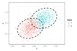
(a) $n=1000$

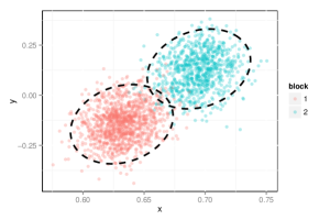
(b) $n=2000$

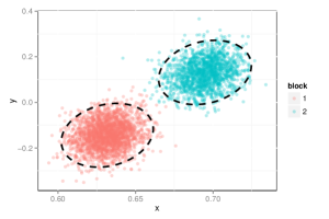
(c) $n=4000$

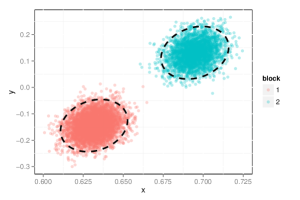
(d) $n=8000$

Figure 1: Plot of the estimated latent positions for $n\in\{1000,2000,4000,8000\}$. Dashed ellipses give the 95% level curves for the distributions as specified in Theorem 4.8.

We then estimate the covariance matrices for the residuals. The theoretical covariance matrices are given in the last line of Table 1, where $\Sigma_{1}$ and $\Sigma_{2}$ are the covariance matrices for the residual $\sqrt{n}(\widehat{X}_{i}-X_{i})$ when $X_{i}$ is from the first block and second block, respectively. The empirical covariance matrices, denoted $\widehat{\Sigma}_{1}$ and $\widehat{\Sigma}_{2}$, are computed by evaluating the sample covariance of the rows of $\sqrt{n}\widehat{X}_{i}$ corresponding to vertices in block 1 and 2 respectively. The estimates of the covariance matrices are given in Table 1. We see that as $n$ increases, the sample covariances tend toward the specified limiting covariance matrix given in the last row.

$n$	2000	4000	8000	16000	$\infty$
$\widehat{\Sigma}_{1}$	$\begin{bmatrix}0.58&0.54\\ 0.54&16.56\end{bmatrix}$	$\begin{bmatrix}0.58&0.63\\ 0.63&14.87\end{bmatrix}$	$\begin{bmatrix}0.60&0.61\\ 0.61&14.20\end{bmatrix}$	$\begin{bmatrix}0.59&0.58\\ 0.58&13.96\end{bmatrix}$	$\begin{bmatrix}0.59&0.55\\ 0.55&13.07\end{bmatrix}$
$\widehat{\Sigma}_{2}$	$\begin{bmatrix}0.58&0.75\\ 0.75&16.28\end{bmatrix}$	$\begin{bmatrix}0.59&0.71\\ 0.71&15.79\end{bmatrix}$	$\begin{bmatrix}0.58&0.54\\ 0.54&14.23\end{bmatrix}$	$\begin{bmatrix}0.61&0.69\\ 0.69&13.92\end{bmatrix}$	$\begin{bmatrix}0.60&0.59\\ 0.59&13.26\end{bmatrix}$

Table 1: The sample covariance matrices for $\sqrt{n}(\widehat{X}_{i}-X_{i})$ for each block in a stochastic blockmodel with two blocks. Here $n\in\{2000,4000,8000,16000\}$. The last column are the theoretical covariance matrices for the limiting distribution.

We also investigate the effects of the multivariate normal distribution as specified in Theorem 4.8 on inference procedures. It is shown in Sussman et al. (2012, 2014) that the approach of embedding a graph into some Euclidean space, followed by inference (for example, clustering or classification) in that space can be consistent. However, these consistency results are, in a sense, only first-order results. In particular, they demonstrate only that the error of the inference procedure converges to $0$ as the number of vertices in the graph increases. We now illustrate how Theorem 4.8 may lead to a more refined error analysis.

We construct a sequence of random graphs on $n$ vertices, where $n$ ranges from $1000$ through $4000$ in increments of $250$, following the stochastic blockmodel with parameters as given above in Eq. (5.1). For each graph $G_{n}$ on $n$ vertices, we embed $G_{n}$ and cluster the embedded vertices of $G_{n}$ via Gaussian mixture model and K-Means. Gaussian mixture model-based clustering was done using the MCLUST implementation of (Fraley and Raftery, 1999). We then measure the classification error of the clustering solution. We repeat this procedure 100 times to obtain an estimate of the misclassification rate. The results are plotted in Figure 2. For comparison, we also plot the Bayes optimal classification error rate under the assumption that the embedded points do indeed follow a multivariate normal mixture with covariance matrices $\Sigma_{1}$ and $\Sigma_{2}$ as given above in the last line of Table 1. We also plot the misclassification rate of $(C\log{n})/n$ as given in Sussman et al. (2012) where the constant $C$ was chosen to match the misclassification rate of $K$-means clustering for $n=1000$. For the number of vertices considered here, the upper bound for the constant $C$ from Sussman et al. (2012) will give a vacuous upper bound of the order of $10^{6}$ for the misclassification rate in this example.

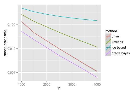
Figure 2: Comparison of classification error for Gaussian mixture model, K-Means, Bayes optimal error rate. The classification errors for each $n\in\{1000,1250,1500,\dots,4000\}$ were obtained by averaging 100 Monte Carlo iterations and are plotted on a $\log_{10}$ scale. The plot indicates that the assumption of mixture of multivariate normals can yield non-negligible improvement in the inference procedure. The log-bound curve shows an upper bound on the error rate as derived in Sussman et al. (2012).

6 Discussion

Our demonstration of the clustering accuracy in § 4 shows how our Theorem 4.8 may impact statistical inference for random graphs. First, we see that the empirical error rates are much lower than those proved in previous work on spectral methods (Rohe et al., 2011; Sussman et al., 2012; Fishkind et al., 2013). Indeed, for both the $K$-Means algorithm and Gaussian mixture model, the average clustering error decreases at an exponential rate as opposed to the $\log(n)/n$ bounds shown in previous work. Furthermore, the rate of decrease for Gaussian mixture model-based clustering closely mirrors the Bayes optimal error rate that would be achieved if the estimated latent positions were exactly distributed according to the multivariate normal distribution and the parameters of this distribution were known.

These results suggest that further investigations using our theorem could lead to much more accurate bounds on the empirical error rates for adjacency spectral clustering. We believe that extending Corollary 4.11 to the case in which $K$ is growing with $n$, e.g., $K=n$, and further work regarding distributions of spectral statistics for stochastic blockmodels will lead to foundational statistical procedures analogous to the results on estimation, hypothesis testing, and clustering in the setting of mixtures of normal distributions in Euclidean space. The relatively simple nature of our spectral procedure allows for computationally efficient statistical methodology.

Extensions of this work to a wider class of exchangeable graphs are also of interest. Though not all exchangeable random graphs can be represented as random dot product graphs, random dot product graphs can approximate any exchangeable graph in the following sense: given a sufficiently regular link function, there exists a feature map from the original latent position space to $\ell_{2}$, such that the link function applied to the original latent positions is equal to the inner product applied to the feature-mapped positions in $\ell_{2}$. Tang et al. (2013) argue that by increasing the dimension of the estimated latent positions, it is possible to estimate these feature-mapped latent positions in a way that allows for consistent subsequent inference. Though this larger class of models is not considered here, we believe this is strong motivation to study the random dot product graph model and its eigenvalues and eigenvectors.

References

• Aldous [1981] D. J. Aldous. Representations for partially exchangeable arrays of random variables. Journal of Multivariate Analysis, 11:581–598, 1981.
• Alon et al. [2002] N. Alon, M. Krivelevich, and V. H. Vu. On the concentration of eigenvalues of random symmetric matrices. Israel Journal of Mathematics, 131:259–267, 2002.
• Bickel and Chen [2009] P. J. Bickel and A. Chen. A nonparametric view of network models and Newman-Girvan and other modularities. Proceedings of the National Academy of Sciences of the United States of America, 106:21068–73, 2009.
• Bickel et al. [2011] P. J. Bickel, A. Chen, and E. Levina. The method of moments and degree distributions for network models. Annals of Statistics, 39:38–59, 2011.
• Bollobás et al. [2007] B. Bollobás, S. Janson, and O. Riordan. The phase transition in inhomogeneous random graphs. Random Structures & Algorithms, 31:3–122, 2007.
• Choi et al. [2012] D. S. Choi, P. J. Wolfe, and E. M. Airoldi. Stochastic blockmodels with a growing number of classes. Biometrika, 99:273–284, 2012.
• Chung [1997] F. R. K. Chung. Spectral Graph Teory. American Mathematical Society, 1997.
• Chung [2001] K. L. Chung. A course in probability theory. Academic Press New York, 3 edition, 2001.
• Diaconis and Janson [2008] P. Diaconis and S. Janson. Graph limits and exchangeable random graphs. Rendiconti di Matematica, 28:33–61, 2008.
• Fiedler [1973] M. Fiedler. Algebraic connectivity of graphs. Czechoslovak Mathematical Journal, 23:298–305, 1973.
• Fishkind et al. [2013] D. E. Fishkind, D. L. Sussman, M. Tang, J. T. Vogelstein, and C. E. Priebe. Consistent adjacency-spectral partitioning for the stochastic block model when the model parameters are unknown. SIAM Journal on Matrix Analysis and Applications, 34:23–39, 2013.
• Fortunato [2010] S. Fortunato. Community detection in graphs. Physics Reports, 486:75–174, 2010.
• Fraley and Raftery [1999] C. Fraley and A. E. Raftery. MCLUST: Software for model-based cluster analysis. Journal of Classification, 16:297–306, 1999.
• Füredi and Komlós [1981] Z. Füredi and J. Komlós. The eigenvalues of random symmetric matrices. Combinatorica, 1:233–241, 1981.
• Goldenberg et al. [2010] A. Goldenberg, A. X. Zheng, S. E. Fienberg, and E. M. Airoldi. A survey of statistical network models. Foundations and Trends® in Machine Learning, 2:129–233, 2010.
• Hoff et al. [2002] P. D. Hoff, A. E. Raftery, and M. S. Handcock. Latent Space Approaches to Social Network Analysis. Journal of the American Statistical Association, 97:1090–1098, 2002.
• Hoover [1979] D. N. Hoover. Relations on probability spaces and arrays of random variables. Technical report, Institute for Advanced Study, 1979.
• Janson [2005] S. Janson. The first eigenvalue of random graphs. Combinatorics, Probability and Computing, 14:815–828, 2005.
• Knowles and Yin [2011] A. Knowles and J. Yin. Eigenvector distribution of wigner matrices. Probability Theory and Related Fields, pages 1–40, 2011.
• Krivelevich and Sudakov [2003] M. Krivelevich and B. Sudakov. The largest eigenvalue of sparse random graphs. Combinatorics, Probability and Computing, 12:61–72, 2003.
• Luxburg [2007] U. Von Luxburg. A tutorial on spectral clustering. Statistics and computing, 17:395–416, 2007.
• Oliveira [2010] R. I. Oliveira. Concentration of the adjacency matrix and of the laplacian in random graphs with independent edges. Arxiv preprint http://arxiv.org/abs/0911.0600, 2010.
• Rohe et al. [2011] K. Rohe, S. Chatterjee, and B. Yu. Spectral clustering and the high-dimensional stochastic blockmodel. Annals of Statistics, 39:1878–1915, 2011.
• Sarkar and Bickel [2013] P. Sarkar and P. J. Bickel. Role or normalization in spectral clustering for stochastic blockmodels. Arxiv preprint. http://arxiv.org/abs/1310.1495, 2013.
• Sussman et al. [2012] D. L. Sussman, M. Tang, D. E. Fishkind, and C. E. Priebe. A consistent adjacency spectral embedding for stochastic blockmodel graphs. Journal of the American Statistical Association, 107:1119–1128, 2012.
• Sussman et al. [2014] D. L. Sussman, M. Tang, and C. E. Priebe. Consistent latent position estimation and vertex classification for random dot product graphs. IEEE Transactions on Pattern Analysis and Machine Intelligence, 36:48–57, 2014.
• Tang et al. [2013] M. Tang, D. L. Sussman, and C. E. Priebe. Universally consistent vertex classification for latent position graphs. Annals of Statistics, 41:1406 – 1430, 2013.
• Tao and Vu [2012] T. Tao and V. Vu. Random matrices: Universal properties of eigenvectors. Random Matrices: Theory and Applications, 1, 2012.
• Tropp [2011] J. A. Tropp. Freedman’s inequality for matrix martingales. Electronic Communications in Probability, 16:262–270, 2011.
• Yan and Xu [2013] T. Yan and J. Xu. A central limit thereom in the $\beta$-model for undirected random graphs with a diverging number of vertices. Biometrika, 100:519–524, 2013.
• Young and Scheinerman [2007] S. Young and E. Scheinerman. Random dot product graph models for social networks. In Algorithms and models for the web-graph, pages 138–149. Springer, 2007.