Local and Global Analysis of Parametric Solid Sweeps

Abstract

In this work, we propose a detailed computational framework for modelling the envelope of the swept volume, that is the boundary of the volume obtained by sweeping an input solid along a trajectory of rigid motions. Our framework is adapted to the well-established industry-standard brep format to enable its implementation in modern CAD systems. This is achieved via a “local analysis”, which covers parametrization and singularities, as well as a “global theory” which tackles face-boundaries, self-intersections and trim curves. Central to the local analysis is the “funnel” which serves as a natural parameter space for the basic surfaces constituting the sweep. The trimming problem is reduced to the problem of surface-surface intersections of these basic surfaces. Based on the complexity of these intersections, we introduce a novel classification of sweeps as either decomposable or non-decomposable. Further, we construct an invariant function $\theta$ on the funnel which efficiently separates decomposable and non-decomposable sweeps. Through a geometric theorem we also show intimate connections between $\theta$, local curvatures and the inverse trajectory used in earlier works as an approach towards trimming. In contrast to the inverse trajectory approach, $\theta$ is robust and is the key to a complete structural understanding, and an efficient computation of both, the singular locus and the trim curves, which are central to a stable implementation. Several illustrative outputs of a pilot implementation are included.

1 Introduction

This paper is motivated by the need for a robust implementation of solid sweeps in solid modeling kernels. The solid sweep is of course, the envelope surface of a solid which is swept in space by a family of rotations and translations. The uses of sweeps are many, e.g., in the design of scrolls [15], in CNC machining verification [12], to detect collisions, and so on. See Appendix for an application of solid sweep in designing scrolls, where we describe a modeling attempt using an existing kernel and its limitations. Constant radius blends can be considered as the partial envelope of a sphere moving along a specified path. As with blends, it is expected that a deeper mathematical understanding of solid sweep will lead to its rapid deployment and use.

A robust implementation of solid sweep poses the following requirements: (i) allow for input models specified in the industry-standard brep format, (ii) output the sweep envelope in the brep format, with effective evaluators, and finally, (iii) perform body-check, i.e., a check on the orientability, non-self-intersection, detection of singularities and so on. Thus there are some “local” parts and some “global” parts to the problem.

It is generally recognized that the harder parts of the local theory is in the smooth case, i.e., when faces meet each other smoothly. For in the non-smooth case, the added complexity in the local geometry of the sweep is exactly that of a curve moving in 3-space. This is of course well understood, and offered by many kernels as a basic surface type. As far as we know, the global situation in the non-smooth case, i.e., the topological structure of edges and vertices (i.e., the 1-cage) of the sweep has not been elucidated, but is also generally assumed to be simpler than the smooth case. In fact, much of existing literature has focused on a smooth single-face solid, as the key problem [1, 3, 4].

In this paper, we focus on the smooth multi-face solid. In Section 2, we start with the mathematical structure of the simple sweep (i.e., one without singularities and self-intersections). By the calculus of curves of contact, we set up a correspondence between the faces, edges and vertices of the envelope with those of the swept solid. This sets up the brep structure of the envelope. Next, we define the funnel as the parametrization space of a face of the envelope and construct a parametrization. We further elucidate the structure of the bounding edges/vertices of a face and provide several examples of simple sweeps from a pilot implementation.

In Section 3, we examine the trim structures. The funnel of Section 2 will remain the ambient parametrization of the faces. The correspondence will help us define the trim areas and trim curves which must be excised to form the correct envelope. We then define the function $\ell$ and use it to define elementary and singular trim curves.

In Section 4, we start with the decomposable sweep, i.e., one which may be partitioned into a suitable small collection of simple sweeps. The final envelope is obtained by stable (transversal) boolean operations on this collection. We show that the trim curves so obtained are elementary. We next define an invariant $\theta$ on the funnels, which is robustly and efficiently computable and we show that $\theta>0$ on (all) the funnels characterizes decomposability. This is an important step in the robust implementation of sweeps.

In Section 5, we prove some of the properties of $\theta$ such as its invariance and show that it is the determinant of the transformation connecting two 2-frames on the envelope, and is thus an easily computable function on the surface. We show that the $\theta=0$ curve on the funnel is also the singular locus for the envelope surface. Via a geometric theorem, we also show that the function $\theta$ matches the one by [4] for implicitly defined surfaces and using the so-called inverse trajectory.

In Section 6, we define the singular trim curve, i.e., where $\ell$ may hit zero. We show that there is a correspondence between singular trim curves and the curves in the zero-locus of $\theta$. We also show that (i) singular trim curves make contact with the $\theta=0$ curves, and (ii) excision at the singular trim curves removes all singularities of the envelope except at these points of contact. Furthermore, these points are easily and robustly computed.

In Section 7 we summarize what has been achieved, viz., that the decomposability and the zero-locus of $\theta$ complement to give a complete understanding of all trim curves. We also discuss some implementation issues and extensions.

Previous work

We now review existing related work. Perhaps the most elaborate proposal for the sweep surface ${\cal E}$ is the sweep envelope differential equations [3] approach, where the authors (i) assume that surface $S$ being swept is implicitly given by a function $f$, and (ii) derive a differential equation whose solution is the envelope. For any point $p$ on the initial curve of contact, a Runge-Kutta marching yields a trajectory $p(t)$ such that (i) $p(0)=p$, and (ii) $p(t)\in{C}(t)$, the curve of contact at time $t$. These trajectories presumably serve as the iso-parametric lines $p(t)={\cal E}(t,u(p))$. Determining whether $p(t)$ is in the trimming set $T$ is solved by using the inverse trajectory condition. This is implemented by using the second derivative of the function $\phi(x,t)=f(\eta(x,t))$, where $\eta$ is the inverse trajectory of point $x$.

On the global front, the building of the envelope ${\cal E}$ is done by selecting a collection of points on the initial curve of contact, developing trajectories, testing for membership in $T$ and then using the points which pass to construct an approximation to the envelope. The drawbacks are clear. Typically, constructing an $f$ which defines $S$ is difficult. Furthermore, the choice of $f$ seems to determine many computational and parametric issues, which is undesirable. The inverse-trajectory check remains poorly conditioned, especially when the second derivative of the function $\phi(x,t)$ w.r.t. $t$ is zero. The structure of the envelope is unknown where this derivative is zero. A global understanding of $T$ and the nature of the trim curves is missing.

In [7], while classifying points for sweeping solids, the authors give a membership test for a point in the object space to belong inside, outside or on the boundary of the swept volume by using inverse trajectory of that point. A curve-solid intersection is required to be computed for each point membership query which is computationally expensive, especially when the intersection is non-transversal, as noted by the authors themselves. Such high degree of computational complexity is prohibitive for a practical implementation.

In [8] the authors work with 2D shapes and 2D motions and quantify singularities using inverse trajectories. This work is based on the computational framework described in [7] and involves computing intersections between 2D curves and 2D shapes. The authors remark that this work can be extended to the 3-dimensional case involving intersections between 3D curves and 3D solids. This approach has the same drawback as [7], namely a high computational cost.

In trimming self-intersections in swept volumes [14], the authors detect self-intersections by computing approximate curves of contact at a few discrete time instances which are then checked for intersections. Approximations are introduced at multiple levels, hence an accurate solution cannot be expected from this method.

2 Mathematical structure of sweeps

In this section we formulate the boundary of the volume obtained by sweeping a solid $M$ along a given trajectory $h$.

2.1 Correspondence and brep structure of envelope

We will use the boundary representation, also known as brep, which is a popular standard for representing a compact and oriented solid $M$ by its boundary $\partial M$. The boundary $\partial M$ separates the interior of $M$ from the exterior of $M$ and is represented using a set of faces, edges and vertices. See Figure 1 for the brep of a solid where different faces are colored differently. Faces meet in edges and edges meet in vertices. The brep consists of two interconnected pieces of information, viz., the geometric and the topological. The geometric information consists of the parametric description of the faces and edges while the topological information consists of orientation of the geometric entities and adjacency relations between them.

In this paper we consider solids whose boundary is formed by faces meeting smoothly. In the case when the faces do not meet smoothly, the added complexity in the local geometry of the sweep is exactly that of a curve moving in 3-space. This is of course well understood, and offered by many kernels as a basic surface type. The global geometry and topology for this case will be described in a later paper.

Definition 1

A trajectory in $\mathbb{R}^{3}$ is specified by a map

$$h:I\rightarrow(SO(3),\mathbb{R}^{3}),h(t)=(A(t),b(t))$$

where $I$ is a closed interval of $\mathbb{R}$, $A(t)\in SO(3),b(t)\in\mathbb{R}^{3}$. The parameter $t$ represents time.

We assume that $h$ is of class $C^{k}$ for some $k\geq 2$, i.e., partial derivatives of order up to $k$ exist and are continuous.

We make the following key assumption about $(M,h)$.

Assumption 2

The tuple $(M,h)$ is in a general position.

Definition 3

The action of $h$ (at time $t$ in $I$) on $M$ is given by $M(t)=\{A(t)\cdot x+b(t)|x\in M\}$. The swept volume ${\cal V}$ is the union $\displaystyle\bigcup_{t\in I}M(t)$ and the envelope ${\cal E}$ is defined as the boundary of the swept volume ${\cal V}$.

Clearly, for each point $y$ of ${\cal E}$ there must be an $x\in M$ and a $t\in I$ such that $y=A(t)\cdot x+b(t)$. This sets up the following correspondence relation.

Definition 4

The correspondence $R$ is the set of tuples

$$R=\{(y,x,t)\in{\cal E}\times M\times I|y=A(t)\cdot x+b(t)\}$$

For $t_{0}\in I$, we set $R_{t_{0}}:=\{(y,x,t)\in R|t=t_{0}\}$. Similarly, for $y_{0}\in{\cal E}$, we define ${{}_{y_{0}}}R:=\{(y,x,t)\in R|y=y_{0}\}$.

We will denote the interior of a set $W$ by $W^{o}$. It is clear that ${\cal V}^{o}=\cup_{t\in I}M(t)^{o}$. Therefore, we have

Lemma 5

If $x\in M^{o}$, then for all $t\in I$, $A(t)\cdot x+b(t)\notin{\cal E}$.

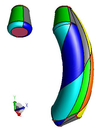
Figure 1: The envelope of a blended cone being swept along a helical trajectory with compounded rotation.

Thus, the points in interior of $M$ do not contribute to ${\cal E}$ at all and $R\subset{\cal E}\times\partial M\times I$. This sets up the brep structure for ${\cal E}$. In the sweep example shown in Figure 1, the correspondence $R$ is illustrated via color coding, i.e., for $(y,x,t)\in R$, the points $y$ and $x$ are shown in the same color. The general position assumption on $(M,h)$ can be formulated as the condition that the induced brep topology of ${\cal E}$ remains invariant under a small perturbation of $(M,h)$.

Lemma 6

Assuming general position of $(M,h)$, for any $y\in{\cal E}$, there are at most three distinct tuples $(y,x_{i},t_{i})$ for $i=1,2,3$ which belong to ${{}_{y}}R$.

Proof. For distinct tuples $(y,x_{1},t_{1}),(y,x_{2},t_{2})\in{{}_{y}}R$, it is clear that $t_{1}\neq t_{2}$, for otherwise $x_{1}=x_{2}$. Therefore $\partial M(t_{1})$ and $\partial M(t_{2})$ intersect at point $y$. By Assumption 2 this intersection is transversal. Further, by the same assumption, at most $3$ surfaces may intersect in a point. $\square$

Definition 7

For a point $x\in M$, define the trajectory of $\boldsymbol{x}$ as the map $\gamma_{x}:I\to\mathbb{R}^{3}$ given by $\gamma_{x}(t)=A(t)\cdot x+b(t)$ and the velocity $v_{x}(t)$ as $v_{x}(t)=\gamma_{x}^{\prime}(t)=A^{\prime}(t)\cdot x+b^{\prime}(t)$.

For a point $x\in\partial M$, let $N(x)$ be the unit outward normal to $M$ at $x$. Define the function $g:\partial M\times I\to\mathbb{R}$ as

$$g(x,t)=\left<A(t)\cdot N(x),v_{x}(t)\right>$$ (1)

Thus, $g(x,t)$ is the dot product of the velocity vector with the unit normal at the point $\gamma_{x}(t)\in\partial M(t)$.

Proposition 8 gives a necessary condition for a point $x\in\partial M$ to contribute a point on ${\cal E}$ at time $t$, namely, $\gamma_{x}(t)$, and is a rewording in our notation of the statement in [3] that the candidate set is the union of the ingress, the egress and the grazing set of points.

Proposition 8

For $(y,x,t)\in R$ and $I=[t_{0},t_{1}]$, either (i) $g(x,t)=0$ or (ii) $t=t_{0}$ and $g(x,t)\leq 0$, or (iii) $t=t_{1}$ and $g(x,t)\geq 0$.

For proof, refer the Appendix.

Definition 9

For a fixed time instant $t_{0}\in I$, the set $\{\gamma_{x}(t_{0})|x\in\partial M,g(x,t_{0})=0\}$ is referred to as the curve of contact at $t_{0}$ and denoted by $C_{I}(t_{0})$. Observe that $C_{I}(t_{0})\subset\partial M(t_{0})$. The union of the curves of contact is referred to as the contact set and denoted by $C_{I}$, i.e., $C_{I}=\displaystyle\bigcup_{t\in I}C_{I}(t)$.

In the sweep example in Figure 4, the curve of contact at $t=0$ is shown imprinted on the solid in red. The curves of contact are referred to as the characteristic curves in [11].

Definition 10

Define projections $\tau:R\to I$ and $Y:R\to{\cal E}$ as: $\tau(y,x,t)=t\mbox{~{}~{}and~{}~{}}Y(y,x,t)=y$.

Definition 11

A sweep $(M,h,I)$ is said to be simple if for all $t\in I^{o}$, $C_{I}(t)=Y(R_{t})$.

Note that, by Proposition 8, for any sweep, we have $Y(R_{t})\subseteq C_{I}(t)$. In a simple sweep, we require that $C_{I}(t)=Y(R_{t})$. In other words, every point on the contact-set appears on the envelope, and thus, no trimming of the contact-set is needed in order to obtain the envelope.

Lemma 12

For a simple sweep, for all $y\in{\cal E}$, ${{}_{y}}R$ is a singleton set.

Proof. We first show that for a simple sweep, for $t\neq t^{\prime}$, $C_{I}(t)\cap C_{I}(t^{\prime})=\emptyset$. Suppose that $y\in C_{I}(t)\cap C_{I}(t^{\prime})$. Clearly, $C_{I}(t)\subset\partial M(t)$ and $C_{I}(t^{\prime})\subset\partial M(t^{\prime})$. Hence $y\in\partial M(t)\cap\partial M(t^{\prime})$. Since $\partial M(t)$ and $\partial M(t^{\prime})$ intersect transversally, $C_{I}(t)\cap M^{o}(t^{\prime})\neq\emptyset$ and $C_{I}(t^{\prime})\cap M^{o}(t)\neq\emptyset$. It follows by Lemma 5 that $C_{I}(t)\not\subset Y(R_{t})$ and $C_{I}(t^{\prime})\not\subset Y(R_{t^{\prime}})$ which contradicts the fact that $(M,h,I)$ is simple.

Now suppose that there are $2$ tuples $(y,x_{i},t_{i})\in{{}_{y}}R$ for $i=1,2$. Since $\partial M$ is free from self-intersections it follows that $t_{1}\neq t_{2}$ and $y\in C_{I}(t_{1})\cap C_{I}(t_{2})$ which is a contradiction to the fact that $(M,h,I)$ is simple. $\square$

2.2 Parametrizations

Now we describe parametrizations of the various entities of the induced brep structure of ${\cal E}$. Here we restrict to the case of the simple sweep. The more general case is derived from this.

2.2.1 Geometry of faces of ${\cal E}$

Let $F$ be a face of ${\partial M}$. In general, $F$ gives rise to multiple faces of ${\cal E}$. Below we describe a natural parametrization of these faces using the parametrization of the surface underlying the face $F$.

Definition 13

A smooth/regular parametric surface in $\mathbb{R}^{3}$ is a smooth map $S:\mathbb{R}^{2}\to\mathbb{R}^{3}$ such that at all $(u_{0},v_{0})\in\mathbb{R}^{2}$ $\frac{\partial S}{\partial u}|_{(u_{0},v_{0})}\in\mathbb{R}^{3}$ and $\frac{\partial S}{\partial v}|_{(u_{0},v_{0})}\in\mathbb{R}^{3}$ are linearly independent. Here $u$ and $v$ are called the parameters of the surface.

Let $S(u,v)$ be the surface underlying the face $F$ of $\partial M$.

Definition 14

Define the function $f:\mathbb{R}^{2}\times I\to\mathbb{R}$ as $f(u,v,t)=g(S(u,v),t)$.

The domain of function $f$ will be referred to as the parameter space. Note that $f$ is easily and robustly computed.

Definition 15

For an interval $I=[t_{0},t_{1}]$, we define the following subsets of the parameter space

$${\cal L} =\{(u,v,t_{0})\in\mathbb{R}^{2}\times\{t_{0}\}\mbox{ such that }f(u,v,t_{0})\leq 0\}$$

$${\cal F} =\{(u,v,t)\in\mathbb{R}^{2}\times I\mbox{ such that }f(u,v,t)=0\}$$

$${\cal R} =\{(u,v,t_{1})\in\mathbb{R}^{2}\times\{t_{1}\}\mbox{ such that }f(u,v,t_{1})\geq 0\}$$

The set ${\cal F}$ will be referred to as the funnel.

Figure 2: The funnel and the contact-set.

By Assumption 2 about the general position of $(M,h)$ it follows that for all $p\in{\cal F}$, the gradient $\nabla f(p)=[f_{u}(p),f_{v}(p),f_{t}(p)]^{T}\neq\bar{0}$. As a consequence, ${\cal F}$ is a smooth, orientable surface in the parameter space.

Definition 16

The set $\{(u,v,t)\in{\cal F}|t=t_{0}\}$ will be referred to as the p-curve of contact at $t_{0}$ and denoted by ${\cal F}(t_{0})$.

We now define the sweep map from the parameter space to the object space.

Definition 17

The sweep map is defined as follows.

$$\sigma:\mathbb{R}^{2}\times I\to\mathbb{R}^{3},\sigma(u,v,t)=A(t)\cdot S(u,v)+b(t)$$

Note that, $\sigma$ is a smooth map, $C_{I}=\sigma({\cal F})$ and $C_{I}(t)=\sigma({\cal F}(t))$. Here and later, by a slight abuse of notation, ${\cal E}$, $C_{I}$ and $C_{I}(t)$ denote the appropriate parts of complete ${\cal E}$, $C_{I}$ and $C_{I}(t)$ respectively resulting from the face $F\subset\partial M$ whose underlying surface is $S$. The surface patches $\sigma({\cal L})$ and $\sigma({\cal R})$ will be referred to as the left and right end-caps respectively.

The funnel, the contact-set, ${\cal F}(t_{0})$ and $C_{I}(t_{0})$ are shown schematically in Figure 2.

The condition $f=0$ can also be looked upon as the rank deficiency condition [1] of the Jacobian $J_{\sigma}$ of the sweep map $\sigma$. To make this precise, let

$$J_{\sigma}=\begin{bmatrix}\sigma_{u}&\sigma_{v}&\sigma_{t}\end{bmatrix}_{3\times 3}$$ (2)

where $\sigma_{u}=A(t)\cdot\frac{\partial S}{\partial u}(u,v)$, $\sigma_{v}=A(t)\cdot\frac{\partial S}{\partial v}(u,v)$ and $\sigma_{t}=A^{\prime}(t)\cdot S(u,v)+b^{\prime}(t)$. Note that if $S(u,v)=x$ then $\sigma_{t}=\gamma_{x}^{\prime}(t)$ is the velocity, also denoted by $V(u,v,t)$. Observe that regularity of $S$ ensures that $J_{\sigma}$ has rank at least 2. Further, it is easy to show that $f(u,v,t)$ is a non-zero scalar multiple of the determinant of $J_{\sigma}$. Therefore, the condition $f=0$ is precisely the rank deficiency condition of $J_{\sigma}$.

For a simple sweep, by Proposition 8, Definition 11 and Definition 15 it follows that ${\cal E}=\sigma({\cal L}\cup{\cal F}\cup{\cal R})$. The surface patches $\sigma({\cal L})$ and $\sigma({\cal R})$ can be obtained from $\partial M$ using Proposition 8 and Definition 15. The trim curve in parameter space for $\sigma({\cal L})$ is given by $f(u,v,t_{0})=0$ and that for $\sigma({\cal R})$ is given by $f(u,v,t_{1})=0$.

We now come to the parametrization of $\sigma({\cal F})$. The non-singularity of $f$ makes ${\cal F}$ an effective parametrization space for $\sigma({\cal F})$. Since time $t$ is a central parameter of the sweep problem and is important in numerous applications, it is useful to have $t$ as one of the parameters of $\sigma({\cal F})$. For most non-trivial sweeps there is no closed form solution for the parametrization of the envelope and we address this problem using the procedural paradigm which is now standard in many kernels and is described in the Appendix. In this approach, a set of evaluators are constructed for the curve/surface via numerical procedures which converge to the solution up to the required tolerance. This has the advantage of being computationally efficient as well as accurate.

Clearly, the bounding edges of the multiple faces resulting from the face $F$ of $\partial M$, are generated by the bounding edges of $F$.

2.2.2 Geometry of edges of ${\cal E}$

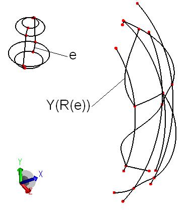
Figure 3: The edges of envelope for the sweep example shown in Figure 1.

We now briefly describe the computation of edges of ${\cal E}$. If $\partial M$ is composed of faces meeting smoothly, an edge $e$ of $\partial M$ will, in general, give rise to a set of edges in ${\cal E}$. We define the restriction of $R$ to the edge $e$ as follows.

Definition 18

For an edge $e\in\partial M$, define $R(e)=\{(y,x,t)\in R|x\in e\}$.

Let $e$ be the intersection of faces $F_{1}$ and $F_{2}$ in $\partial M$ and let $s$ denote the parameter of $e$. Since $F_{1}$ and $F_{2}$ meet smoothly at $e$, at every point $e(s)$ of $e$ there is a well-defined normal. Hence we may define the following function on the parameter space $\mathbb{R}\times I$.

Definition 19

Define the function $f^{e}:\mathbb{R}\times I\to\mathbb{R}$ as $f^{e}(s,t)=g(e(s),t)$.

Note that the function $f^{e}$ is the restriction of the function $f$ defined in Definition 14 to the parameter space curve $(u(s),v(s))$ corresponding to the edge $e$ so that $e(s)=S(u(s),v(s))$ where $S$ is the surface underlying face $F_{1}$. The following Lemma gives a necessary condition for a point $e(s)$ to be on ${\cal E}$ at time $t$.

Lemma 20

For $(y,e(s),t)\in R(e)$ and $I=[t_{0},t_{1}]$, either (i) $t=t_{0}$ and $f^{e}(s,t)\leq 0$, or (ii) $t=t_{1}$ and $f^{e}(s,t)\geq 0$, or (iii) $f^{e}(s,t)=0$.

Proof. This follows from Prop. 8 and Definition 19. $\square$ Figure 3 shows the edges of the envelope for the sweep example shown in Figure 1. The correspondence for one of the edges of the envelope is also marked.

Let ${\cal F}_{1}$ denote the funnel corresponding to the contact set generated by face $F_{1}$. The edge in parameter space which bounds ${\cal F}_{1}$ is given by $\{(u(s),v(s),t)\in\mathbb{R}^{2}\times I|f^{e}(s,t)=0\}$ which we will denote by ${\cal F}^{e}$. Note that ${\cal F}^{e}$ is smooth if $(f^{e}_{s},f^{e}_{t})=(f_{u}\cdot u_{s}+f_{v}\cdot v_{s},f_{t})\neq(0,0)$ at all points in ${\cal F}^{e}$.

2.2.3 Geometry of vertices of ${\cal E}$

A vertex $z$ on ${\partial M}$ will, in general, give rise to a set of vertices on ${\cal E}$. We further restrict the correspondence $R$ to $z$ as $R(z)=\{(y,x,t)\in R|x=z\}$. As $\partial M$ is smooth, there is a well-defined normal at $z$. Hence we may define the function $f^{z}:I\to\mathbb{R}$ as $f^{z}(t)=g(z,t)$. If $z$ is on the boundary of a face $F_{1}$, $z$ will have a set of coordinates in the parameter space of the surface $S$ underlying the face $F_{1}$, say $(u_{0},v_{0})$, so that $z=S(u_{0},v_{0})$. It is easy to see that if $(y,z,t)\in R(z)$ and $I=[t_{0},t_{1}]$ then either (i) $t=t_{0}$ and $f^{z}(t)\leq 0$, or (ii) $t=t_{1}$ and $f^{z}(t)\geq 0$, or (iii) $f^{z}(t)=0$.

2.3 Examples of simple sweeps

Three examples of simple sweeps are shown in Figures 4, 5 and 6 which were generated using a pilot implementation of our algorithm in ACIS 3D Modeler [2]. A curve of contact at initial time is shown imprinted on the solid in Figure 4.

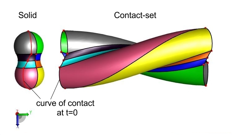
Figure 4: The envelope(without end-caps) of a dumbbell undergoing translation along $y$-axis and undergoing rotation about $y$-axis.

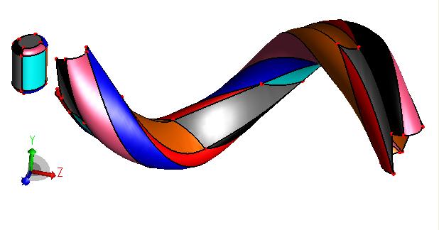
Figure 5: The envelope(without end-caps) of an elliptical cylinder undergoing a screw motion while rotating about its own axis.

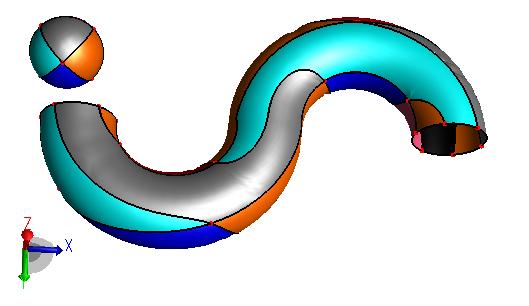
Figure 6: The envelope(without end-caps) of a sphere sweeping along an ’S’ shaped trajectory while rotating about $y$-axis

3 The trim structures

Unlike in a simple sweep, all points of $C_{I}$ may not belong to the envelope. We now define the subset of $C_{I}$ which needs to be excised in order to obtain ${\cal E}$.

Definition 21

The trim set is defined as

$$T_{I}:=\{x\in C_{I}|\exists t\in I,x\in M^{o}(t)\}$$

Lemma 22

The set $T_{I}$ is open in $C_{I}$.

Proof. Consider a point $y_{0}\in T_{I}$. Then $y_{0}\in M^{o}(t_{0})$ for some $t_{0}\in I$. Hence, there exists an open ball of non-zero radius $r$ centered at $y_{0}$, denote it by $B(y_{0},r)$, which is itself contained in $M^{o}(t_{0})$. Let ${\cal N}_{0}:=B(y_{0},r)\cap C_{I}$. Then, ${\cal N}_{0}\subset T_{I}$ and ${\cal N}_{0}$ is open in $T_{I}$. Hence $T$ is open in $C_{I}$. $\square$

In general, the trim set will span several parts of $C_{I}$ corresponding to different faces of $\partial M$. For the ease of notation and presentation, in the rest of this paper, we will analyse the corresponding trim structures on the funnel of a fixed face $F$ of $\partial M$. Thanks to the natural parametrizations (cf. subsection 2.2), the migration of these trim structures across different funnels is an easy implementation detail. In view of this, we carry forward the notation developed in subsection 2.2.1 through the rest of this paper.

Definition 23

The pre-image of $T_{I}$ on the funnel under the map $\sigma$ will be referred to as the p-trim set, denoted by $pT_{I}$, i.e., $pT_{I}=\sigma^{-1}(T_{I})\cap{\cal F}$.

An immediate corollary of Lemma 22 is: $pT_{I}$ is open in ${\cal F}$.

One can also define similar parametric trim areas on the left and right caps (cf. ${\cal L}$ and ${\cal R}$ from Definition 15) and their counterparts in the object space. However, for want of space, we assume here that these trim structures are empty. Our analysis can be extended to also cover the non-empty case.

Definition 24

The boundary of $\overline{T_{I}}$ will be referred to as the trim curves and denoted by $\partial T_{I}$. Here $\overline{T_{I}}$ denotes the closure of $T_{I}$ in $C_{I}$. Similarly, the boundary of the closure $\overline{pT_{I}}$ of $pT_{I}$ in ${\cal F}$ will be referred to as the p-trim curves and denoted by $\partial pT_{I}$.

Note that ${\cal E}\cap T_{I}=\emptyset$, ${\cal E}\cap\overline{T_{I}}=\partial T_{I}$ and $\sigma({\cal F}\setminus pT_{I})={\cal E}$. Therefore the problem of excising the trim set is reduced to the problem of computing the trim curves. Further, this computation is eventually reduced to guided parametric surface-surface intersections via the parametrization of $\sigma({\cal F})$ described in subsection 2.2.

For each point $y\in\partial T_{I}$ there is a finite set of points $p_{i}\in\partial pT_{I}$ such that $\sigma(p_{i})=y$ for all $i$ (cf. Lemma 6). Figure 7 schematically illustrates p-trim curves on ${\cal F}$. For every point $p_{1}$ in the red portion of $\partial pT_{I}$, there is a point $p_{1}^{\prime}$ in the green portion of $\partial pT_{I}$ such that $\sigma(p_{1})=\sigma(p_{1}^{\prime})$.

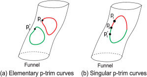
Figure 7: Elementary and singular p-trim curves.

We extend the correspondence of Definition 4 to $C_{I}\times M\times I$ as below. Abusing notation, henceforth, $R$ will denote this correspondence.

Definition 25

Let $R:=\{(y,x,t)\in C_{I}\times M\times I|y=A(t)\cdot x+b(t)\}$. As expected, we define $\tau:R\to I$ and $Y:R\to C_{I}$ as: $\tau(y,x,t)=t\mbox{~{}~{}and~{}~{}}Y(y,x,t)=y$. Further, as before, $R_{t_{0}}:=\{(y,x,t)\in R|t=t_{0}\}$,​ ${{}_{y_{0}}}\!R:=\{(y,x,t)\in R|y=y_{0}\}$.

A crucial observation is that, unlike the earlier correspondence, $R\not\subset C_{I}\times\partial M\times I$.

Definition 26

For $p=(u,v,t)\in{\cal F}$, let $\sigma(p)=y$. Let $L(p):=\tau({{}_{y}}R)$. Define the function $\ell:{\cal F}\to\mathbb{R}\cup\infty$ as follows.

$$\ell(p) =\displaystyle\inf_{t^{\prime}\in L(p)\setminus\{t\}}\|t-t^{\prime}\| \text{ if }L(p)\neq\{t\}$$

$$=\infty \text{ if }L(p)=\{t\}$$

Further, we define $,=\displaystyle\inf_{p\in{\cal F}}\ell(p)$.

For $p\in{\cal F}$, $L(p)$ is the set of all time instances $t^{\prime}$ (except $t$) such that some point of $M(t^{\prime})$ coincides with $\sigma(p)$. Further, the function $\ell$ gives the ‘smallest’ time $\delta t$ such that some point of $M(t\pm\delta t)$ coincides with $\sigma(p)$.

Lemma 27

Let $p_{0}\in\overline{pT_{I}}$. Then $p_{0}\in pT_{I}$ iff $L(p_{0})$ contains an interval, and $p_{0}\in\partial pT_{I}$ iff $L(p_{0})$ is a discrete set of cardinality either two or three.

Proof. Suppose first that $p_{0}\in pT_{I}$. Let $y_{0}:=\sigma(p_{0})$. Then $y_{0}\in T_{I}$ and $y_{0}\in M^{o}(t_{0})$ for some $t_{0}\in I$. Let $B(y_{0},r)$ be an open ball of radius $r>0$ centered at $y_{0}$ contained in $M^{o}(t_{0})$. Assume without loss of generality that $A(t_{0})=I$ and $b(t_{0})=0$. By continuity of the trajectory $h$ it follows that given $r>0$ there exists $\delta t>0$ such that $\|y_{0}-A(t_{0}+\delta t)\cdot y_{0}-b(t_{0}+\delta t)\|<r$. Hence, $y_{0}\in M^{o}(t)$ for all $t\in[t_{0},t_{0}+\delta t]$. In other words, $[t_{0},t_{0}+\delta t]\in L(p_{0})$.

Conversely, suppose that $L(p_{0})$ contains an interval $[t_{1},t_{2}]$, i.e., $y_{0}\in M(t)$ for all $t\in[t_{1},t_{2}]$. By Assumption 2 about the general position of $(M,h)$ it follows that $y_{0}\in M^{o}(t)$ for some $t\in[t_{1},t_{2}]$, i.e., $y_{0}\in T_{I}$ and $p_{0}\in pT_{I}$. We have shown that for $p_{0}\in\overline{pT_{I}}$, $p_{0}\in pT_{I}$ iff $L(p_{0})$ contains an interval. Hence, $L(p_{0})$ is discrete iff $p_{0}\in\partial pT_{I}$.

As $\partial T_{I}\subset{\cal E}$, by Lemma 6, it follows that at all but finitely many points $p\in\partial pT_{I}$, $L(p)$ is of cardinality $2$ and at remaining points it is of cardinality $3$. $\square$

We classify trim curves as follows.

Definition 28

A curve $C$ of $\partial pT_{I}$ is said to be elementary if there exists $\delta>0$ such that for all $p\in C$, $\ell(p)>\delta$. It is said to be singular if $\displaystyle\inf_{p\in C}\ell(p)=0$.

Figures 7(a) and 7(b) schematically illustrate elementary and singular p-trim curves on ${\cal F}$ respectively. Further observe that, $,>0$ in case (a) and 0 in case (b).

Before proceeding further, we introduce the following notation: for $J\subset I$, ${\cal F}(J)=\{(u,v,t)\in{\cal F}\mid t\in J\}$.

Lemma 29

All but finitely many points of elementary trim curves lie on the transversal intersections of two surface patches $\sigma({\cal F}(I_{i}))$ and the remaining points lie on the transversal intersection of three surface patches $\sigma({\cal F}(I_{i}))$ where, for $i=1,2,3$, $I_{i}\subset I$ are subintervals.

Proof. Suppose that all curves of $\partial pT_{I}$ are elementary, i.e., $\exists\delta>0$ such that for all $p\in\partial pT_{I}$, $\ell(p)>\delta$. By Lemma 27, all but finitely many points $y\in\partial T_{I}$ have two points $p_{1}=(u_{1},v_{1},t_{1})$ and $p_{2}=(u_{2},v_{2},t_{2})$ in $\partial pT_{I}$ such that $\sigma(p_{1})=\sigma(p_{2})=y$. Let ${\cal F}_{1}:={\cal F}([t_{1}-\delta,t_{1}+\delta])$ and ${\cal F}_{2}:={\cal F}([t_{2}-\delta,t_{2}+\delta])$. Then $y\in\sigma({\cal F}_{1})\cap\sigma({\cal F}_{2})$. From Section 5.2 we know that $\partial M(t_{1})$ and $\partial M(t_{2})$ are tangential to $\sigma({\cal F}_{1})$ and $\sigma({\cal F}_{2})$ respectively at $y$. By Assumption 2 about general position of $(M,h)$, $\partial M(t_{1})$ and $\partial M(t_{2})$ intersect transversally at $y$. Hence, $\sigma({\cal F}_{1})$ and $\sigma({\cal F}_{2})$ intersect transversally at $y$.

At most finitely many points $y\in\partial T_{I}$ have three points $p_{1},p_{2}$ and $p_{3}$ in $\partial pT_{I}$ such that $\sigma(p_{i})=y$. By an argument similar to above, it can be shown that $y$ lies on the transversal intersection of three surface patches $\sigma({\cal F}_{i})$ for ${\cal F}_{i}$ corresponding to appropriate subintervals $I_{i}\subset I$. $\square$

Figure 8 shows an example in which a capsule is swept along a helical path while rotating about $y$-axis. The trim curves are elementary.

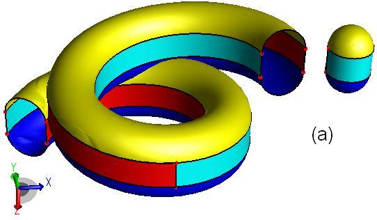
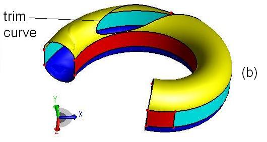
Figure 8: (a) The contact set of a capsule moving along a helix while rotating about $y$-axis.(b) The contact set restricted to interval $[0.5,1.0]$ with the trim set excised.

4 Decomposable sweeps

We now consider sweeps, which though not simple, can be divided into simple sweeps by partitioning the sweep interval so that the trim curves can be obtained by transversal intersections of the contact sets of the resulting simple sweeps. Given an interval $I$, we call a partition ${\cal P}$ of $I$ into consecutive intervals $I_{1},I_{2},\ldots,I_{k_{\cal P}}$ to be of width $\delta$ if $max\{length(I_{1}),length(I_{2}),\ldots,length(I_{k_{\cal P}})\}=\delta$.

Definition 30

We say that the sweep $(M,h,I)$ is decomposable if there exists $\delta>0$ such that for all partitions ${\cal P}$ of $I$ of width $\delta$, each sweep $(M,h,I_{i})$ is simple for $i=1,\cdots,k_{\cal P}$. A sweep which is not decomposable is called non-decomposable.

Figure 9 schematically illustrates the difference between decomposable and non-decomposable sweeps. The example shown in Figure 8 is of a decomposable sweep in which partitioning the sweep interval $I$ into 2 equal halves will result in 2 simple sweeps.

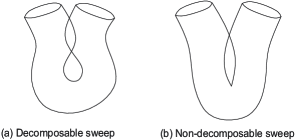
Figure 9: Contact-sets of decomposable and non-decomposable sweeps.

Proposition 31

The sweep $(M,h,I)$ is decomposable iff $,>0$. Further, if $,>0$ then all the p-trim curves are elementary.

Proof. Suppose first that $,>0$. Let ${\cal P}$ be a partition of $I$ of width ,. We show that $(M,h,I_{i})$ is simple for $i=1,2,\ldots,k_{\cal P}$. Let ${\cal E}_{i}$ and $C_{I_{i}}$ be the envelope and the contact set for $(M,h,I_{i})$ respectively. By Proposition 8, (modulo end-caps), ${\cal E}_{i}\subset C_{I_{i}}$. It needs to be shown that $C_{I_{i}}\subset{\cal E}_{i}$. Suppose not. Let $y\in C_{I_{i}}(t)$ such that $y\notin{\cal E}_{i}$ for some $t\in I_{i}$. Then, $y\in T_{I_{i}}$, i.e., $y\in M^{o}(t^{\prime})$ for some $t^{\prime}\in I_{i}$. Let $y=\sigma(p)$ for $p=(u,v,t)$. It follows that $\ell(p)<\|t-t^{\prime}\|\leq length(I_{i})\leq,$, leading to a contradiction. Hence, $(M,h,I)$ is decomposable.

Suppose now that $(M,h,I)$ is decomposable with width-parameter $\delta$ (cf. Definition 30). Consider a point $p_{0}=(u_{0},v_{0},t_{0})\in{\cal F}$ and let $\sigma(p_{0})=y_{0}$. Let $I_{1}=[t_{0}-\delta,t_{0}]$ and $I_{2}=[t_{0},t_{0}+\delta]$. Further, let ${\cal E}_{i}$ and $C_{I_{i}}$ be the envelope and contact-set for the sweeps $(M,h,I_{i})$ respectively. Observe that $y_{0}\in C_{I_{i}}$ for $i=1,2$. Let ${{}_{y_{0}}}R^{i}=\{(y,x,t)\in C_{I_{i}}\times M\times I_{i}|y=y_{0}\}$. As $(M,h,I)$ is decomposable with width-parameter $\delta$, both $(M,h,I_{1})$ and $(M,h,I_{2})$ are simple, and hence, $C_{I_{i}}\subset{\cal E}_{i}$ for $i=1,2$. Therefore, $y_{0}$ belongs to ${\cal E}_{1}$ and ${\cal E}_{2}$. By Lemma 12, ${{}_{y_{0}}}R^{1}$ and ${{}_{y_{0}}}R^{2}$ are both singleton sets. Further, ${{}_{y_{0}}}R^{1}={{}_{y_{0}}}R^{2}=\{(y_{0},x,t_{0})\}$ for $x=S(u_{0},v_{0})\in\partial M$. Hence, $\ell(p_{0})>\delta$. Since for all $p\in{\cal F}$, $\ell(p)>\delta$, we conclude that $,\geq\delta>0$.

Suppose that $,>0$. Since $\ell(p)\geq,$ for all $p\in\partial pT_{I}$ if follows that all the p-trim curves are elementary. $\square$

The above proposition provides a natural test for decomposability. Further, coupled with Lemma 29, for a decomposable sweep, the problem of excising the trim set can be reduced to transversal intersections. However, note that, the very definition of , is post-facto as it relies on the trim structures. Besides, it is the infimum value of the not necessarily continuous function $\ell$ and is difficult to compute. Thus, the above test of decomposability is not effective.

One of the key contributions of this paper is a novel geometric ‘invariant’ function on the funnel which is computed in closed form and serves the following objectives.

1. Quick/efficient and simple detection of decomposability of sweeps, which occur most often in practice.

2. Generation of trim curves for non-decomposable sweeps.

3. Quantification and detection of singularities on the envelope.

For a point $p=(u,v,t)\in\mathcal{F}$, let $q=\sigma(p)$. Recall from subsection 2.2 that, $J_{\sigma}(p)=[\sigma_{u}\sigma_{v}\sigma_{t}]$ is of rank 2. As $det(J_{\sigma}(p))=0$, $\{\sigma_{u}(p),\sigma_{v}(p),\sigma_{t}(p)\}$ are linearly dependent. Recall that $\sigma_{t}(p)=V(p)$ is the velocity of the point $S(u,v)$ at time $t$ (cf. subsection 2.2). As $S$ is regular, the set $\{\sigma_{u}(p),\sigma_{v}(p)\}$ forms a basis for the tangent space to $\partial M(t)$. Therefore, we must have $\sigma_{t}(p)=l(p).\sigma_{u}(p)+m(p).\sigma_{v}(p)$ where $l$ and $m$ are well-defined (unique) on the funnel and are themselves continuous functions on the funnel.

Definition 32

The function $\theta:{\cal F}\to\mathbb{R}$ is defined as follows.

$$\theta(p)=l(p).f_{u}(p)+m(p).f_{v}(p)-f_{t}(p)$$ (3)

where $f_{u},f_{v}$ and $f_{t}$ denote partial derivatives of the function $f$ w.r.t. $u,v$ and $t$ respectively at $p$, and $l$ and $m$ are as defined before.

Note that, unlike $\ell$, $\theta$ is easily and robustly computable continuous function on the funnel. Now we are ready to state one of the main theorems of this paper.

Theorem 33

If for all $p\in{\cal F}$, $\theta(p)>0$, then the sweep is decomposable. Further, if there exists $p\in{\cal F}$ such that $\theta(p)<0$, then the sweep is non-decomposable.

The proof is given in Section 5.6 which highlights many other surprisingly strong properties of the function $\theta$.

Definition 34

The function $\theta$ partitions the funnel ${\cal F}$ into three sets, viz. (i) ${\cal F}^{+}:=\{p\in{\cal F}|\theta(p)>0\}$, (ii) ${\cal F}^{-}:=\{p\in{\cal F}|\theta(p)<0\}$ and (iii) ${\cal F}^{0}:=\{p\in{\cal F}|\theta(p)=0\}$. Further, we define ${C_{I}}^{+}:=\sigma({\cal F}^{+})$, ${C_{I}}^{-}:=\sigma({\cal F}^{-})$ and ${C_{I}}^{0}:=\sigma({\cal F}^{0})$.

Figure 10 schematically illustrates the sets ${\cal F}^{+},{\cal F}^{-}$ and ${\cal F}^{0}$ on the funnel and sets ${C_{I}}^{-},{C_{I}}^{+}$ and ${C_{I}}^{0}$.

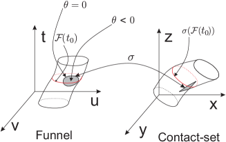
Figure 10: The shaded region on ${\cal F}$ and $C_{I}$ corresponds to ${\cal F}^{-}$ and ${C_{I}}^{-}$ respectively. A curve of contact is shown in red.

Note that, for $(M,h,I)$ in general position, either ${\cal F}^{-}$ is a non-empty open set or ${\cal F}={\cal F}^{+}$. Whence, the above theorem provides an efficient ‘open’ test for decomposability, namely, a sweep $(M,h,I)$ is decomposable iff the open set ${\cal F}^{-}$ is empty. Most kernels will have an effective procedure for such a test provided $\theta$ is effectively computable.

5 Properties of the invariant $\theta$

In this section we prove some key properties of $\theta$, namely, its invariance under the re-parametrization of the surface being swept and its relation with the notion of inverse trajectory used in earlier works. Finally, we use these properties along with Proposition 31, to prove Theorem 33.

5.1 Invariance of $\theta$

We show that the function $\theta$ is invariant of the parametrization of $\partial M$ and hence, intrinsic to the sweep.

Theorem 35

If $\bar{S}$ is a re-parametrization of the surface $S$ so that $q:=\bar{S}(\bar{u},\bar{v})=S(u,v)$, and $g(q,t)=0$, then $\theta(u,v,t)=\bar{\theta}(\bar{u},\bar{v},t)$.

Proof. Suppose as before that the boundary $\partial M$ is specified by the parametrized surface $S$. Let $\phi:\mathbb{R}^{2}\to\mathbb{R}^{2}$ be a re-parametrization map of $S$ and $\bar{S}:=S\circ\phi$. Since $\phi$ is a diffeomorphism, $d\phi$ is an isomorphism at every point in the entire domain of $\phi$. Let $\phi(\bar{u},\bar{v})=(u(\bar{u},\bar{v}),v(\bar{u},\bar{v}))$. For convenience of expression, we extend $\phi$ to define it on the parameter space of the sweep map $\sigma$ so that $\phi(\bar{u},\bar{v},t)=(u,v,t)$. Hence the re-parametrized sweep map (for $\bar{S}$) is simply $\bar{\sigma}=\sigma\circ\phi$. Recall that $f(u,v,t)=\left<\hat{N}(u,v,t),V(u,v,t)\right>$, where $\hat{N}(u,v,t)$ is the unit outward normal to $\partial M(t)$ at the point $A(t)\cdot S(u,v)+b(t)$. It is easy to check that $\hat{N}(u,v,t)$ can also be expressed as $A(t)\cdot(\mathcal{G}\circ S)(u,v)$, where $\mathcal{G}:\partial M\to S^{2}$ is the intrinsic Gauss map, $S^{2}$ being the unit sphere and $\circ$ stands for the usual composition of functions. Thus,

$$f(u,v,t) =\left<\hat{N}(u,v,t),V(u,v,t)\right>$$

$$=\left<A(t)\cdot(\mathcal{G}\circ S)(u,v),V(u,v,t)\right>$$

Similarly, computing with the re-parametrization $\bar{S}$, and using the fact that $\bar{S}=S\circ\phi$, we have $\bar{f}=f\circ\phi$. Differentiating w.r.t. $\bar{u},\bar{v}$ and $t$ we get $\nabla\bar{f}=d\phi^{T}\cdot\nabla f$ where $d\phi$ is the Jacobian of the map $\phi$.

Observe that, from Eq. 3, for $\bar{p}=(\bar{u},\bar{v},t)$ and $p=\phi(\bar{p})=(u,v,t)$, $\theta(p)=\left<\nabla f(p),z\right>$ where $z=(l,m,-1)$ spans the null-space of $J_{\sigma}|_{p}$ for $p\in\mathcal{F}$. In order to compute $\bar{z}$ for the re-parametrized sweep we see that $J_{\bar{\sigma}}=J_{\sigma}\circ d\phi$ and $\bar{z}=d\phi^{-1}z$. Now using $\nabla\bar{f}=d\phi^{T}\cdot\nabla f$, we get that

$$\bar{\theta}(\bar{p}) =\left<\nabla\bar{f}(\bar{p}),\bar{z}\right>=\left<d\phi^{T}\cdot\nabla f(p),d\phi^{-1}\cdot z\right>$$

$$=\left<\nabla f(p),z\right>=\theta(p)$$

This proves the theorem. $\square$

An important corollary of the above theorem is that the function $\theta$ on the funnel is a pull-back of an intrinsic function, say $\Theta$, on the abstract smooth manifold ${\cal C}_{I}=\cup_{t\in I}C_{I}(t)\times\{t\}$. More precisely, for $p=(u,v,t)\in{\cal F}$ with $\sigma(p)=y\in C_{I}(t)$, define $\Theta((y,t))=\theta(p)$. Then $\Theta$ remains invariant under a re-parametrization. Observe that, unlike ${\cal C}_{I}$, in general, $C_{I}$ is not a smooth manifold.

5.2 Geometric meaning of $\theta$

For a smooth point $w$ of $W$, let ${\cal T}_{W}(w)$ denote the tangent space to $W$ at $w$.

We show that the function $\theta$ arises out of the relation between two 2-frames on ${\cal T}_{C_{I}}$. Let $p=(u,v,t)\in\mathcal{F}$ be such that $\sigma(p)$ is a smooth point of $C_{I}$. We first compute a natural 2-frame ${\cal X}(p)$ in $\mathcal{T}_{\mathcal{F}}(p)$. Note that, $\mathcal{F}$ being the zero level-set of the function $f$, $\nabla f|_{p}\bot\mathcal{T}_{\mathcal{F}}(p)$. We set $\beta:=(-f_{v},f_{u},0)$ and note that $\beta\bot\nabla f$. It is easy to see that $\beta$ is tangent to the p-curve-of-contact $\mathcal{F}(t)$. Let $\alpha:=\nabla f\times\beta=(-f_{u}f_{t},-f_{v}f_{t},f_{u}^{2}+f_{v}^{2})$. Here $\times$ is the cross-product in $\mathbb{R}^{3}$. Clearly, the set $\{\alpha,\beta\}$ forms a basis of $\mathcal{T}_{\mathcal{F}}(p)$ if $(f_{u},f_{v})\neq(0,0)$. Since $\nabla f\neq 0$, if $(f_{u},f_{v})=(0,0)$ then $f_{t}\neq 0$ and $\{\alpha^{\prime},\beta^{\prime}\}:=\{(1,0,0),(0,f_{t},0)\}$ serves as a basis for $\mathcal{T}_{\mathcal{F}}(p)$. Figure 2 illustrates the basis $\{\alpha,\beta\}$ schematically.

The set $\{J_{\sigma}\cdot\alpha,J_{\sigma}\cdot\beta\}\subseteq{\cal T}_{C_{I}}(\sigma(p))$ and can be expressed in terms of $\{\sigma_{u},\sigma_{v}\}$ as follows

$$\begin{bmatrix}J_{\sigma}\cdot\alpha&J_{\sigma}\cdot\beta\end{bmatrix}=\begin{bmatrix}\sigma_{u}&\sigma_{v}\end{bmatrix}\underbrace{\begin{bmatrix}-f_{t}f_{u}+l(f_{u}^{2}+f_{v}^{2})&-f_{v}\\ -f_{t}f_{v}+m(f_{u}^{2}+f_{v}^{2})&f_{u}\end{bmatrix}}_{\mathcal{D}(p)}$$

Note that,

$$det(\mathcal{D}(p)) =(f_{u}^{2}+f_{v}^{2})(lf_{u}+mf_{v}-f_{t})$$ (4)

$$=(f_{u}^{2}+f_{v}^{2})\theta(p)$$ (5)

Clearly, if $(f_{u},f_{v})\neq(0,0)$ then $det(\mathcal{D}(p))$ is a positive scalar multiple of $\theta(p)$. Again, if $(f_{u},f_{v})=(0,0)$, expressing $\{J_{\sigma}\cdot\alpha^{\prime},J_{\sigma}\cdot\beta^{\prime}\}$ in terms of $\{\sigma_{u},\sigma_{v}\}$ we see that $det(\mathcal{D}(p))=\theta(p)=-f_{t}$.

The above relation between $\{\sigma_{u},\sigma_{v}\}$ and $\{J_{\sigma}\cdot\alpha,J_{\sigma}\cdot\beta\}$ shows that if $\theta(p)\neq 0$, then for $y=\sigma(p)$, ${\cal T}_{C_{I}}(y)$ and ${\cal T}_{\partial M(t)}(y)$ are identitical (as subspaces of ${\mathbb{R}}^{3}$), i.e., $\partial M(t)$ makes tangential contact with $C_{I}$ at $y$.

5.3 Non-singularity of $\theta$

We give a sweep example which will demonstrate the non-singularity of the function $\theta$. We show that on the set ${\cal F}^{0}$, $\nabla\theta\neq 0$. Consider a sphere parametrized as $S(u,v)=(\cos v\cos u,\cos v\sin u,\sin v)$, $v\in[-\frac{\pi}{2},\frac{\pi}{2}],u\in[-\pi,\pi]$ swept along a curvilinear trajectory given by $h(t)=(A(t),b(t))$, $A(t)=I,b(t)=(\frac{1}{2}\cos 2t,\frac{1}{2}\sin 2t,0)$, $t\in[0,1]$. The unit outward normal at $S(u,v)$ at time $t$ is given by $\hat{N}(u,v,t)=(\cos v\cos u,\cos v\sin u,\sin v)$ and velocity is given by $V(u,v,t)=(-\sin 2t,\cos 2t,0)$. The envelope function is $f(u,v,t)=\left<\hat{N}(u,v,t),V(u,v,t)\right>=\cos v\sin(u-2t)$. The funnel ${\cal F}$ is given by (i) $u=2t-\pi$, $v\in[-\frac{\pi}{2},\frac{\pi}{2}]$ and (ii) $u=2t$, $v\in[-\frac{\pi}{2},\frac{\pi}{2}]$. Hence, $u$ and $v$ can serve as local parameters of ${\cal F}$. In component (ii) of the funnel, we see that $\theta>0$, hence we will only consider component (i). On ${\cal F}$, $\sigma_{t}=l\sigma_{u}+m\sigma_{v}$ where $l=\frac{-1}{\cos v}$ and $m=0$, whence, $\theta(u,v,t)=lf_{u}+mf_{v}-f_{t}=2\cos v-1$. The set ${\cal F}^{0}$ is given by $v=\pm\frac{\pi}{3}$, $u=2t-\pi$. On ${\cal F}^{0}$, $\frac{\partial\theta}{\partial u}=0$ and $\frac{\partial\theta}{\partial v}=2\sin v\neq 0$.

An important consequence of non-singularity of $\theta$ is that its zero set, i.e., ${\cal F}^{0}$ can be computed robustly and easily.

5.4 Detecting singularities on the envelope

Now we characterize the cusp-singular points of $C_{I}$. Geometrically, these are precisely the points where $C_{I}$ intersects itself non-transversally. Note that, the transversal singularities of $C_{I}$ are addressed through decomposability. We consider the following restriction of $\sigma$ to the funnel: $\sigma|_{\cal F}:{\cal F}\rightarrow{\mathbb{R}}^{3}$. Note that $\sigma|_{\cal F}({\cal F})=C_{I}$.

Definition 36

The set $C_{I}$ is said to have a cusp-singularity at a point $\sigma(p)=x\in C_{I}$ if $\sigma|_{{\cal F}}$ fails to be an immersion at $p$.

A basic result about immersion (see [6]) implies that if $\sigma|_{\cal F}$ is an immersion at a point $p$, then there is a neighborhood ${\cal N}$ of $p$ such that $\sigma|_{\cal F}$ is a local diffeomorphism from ${\cal N}$ onto its image.

Lemma 37

Let $p_{0}\in{\cal F}$ and $\sigma(p_{0})=x_{0}$. The point $x_{0}$ is a cusp-singularity iff $\theta(p_{0})=0$.

Proof. From subsection 5.2, $\theta(p_{0})$ is a positive multiple of the determinant relating frames $\{\sigma_{u},\sigma_{v}\}$ and $\{J_{\sigma}\cdot\alpha,J_{\sigma}\cdot\beta\}$ at $x_{0}$ . Since the set $\{\sigma_{u},\sigma_{v}\}$ is always linearly independent, it follows that $\{J_{\sigma}\cdot\alpha,J_{\sigma}\cdot\beta\}$ is linearly dependent iff $\sigma|_{{\cal F}}$ fails to be an immersion at $p_{0}$ iff $\theta(p_{0})=0$. $\square$

In other words, the set ${C_{I}}^{0}$ is the set of cusp-singular points in $C_{I}$.

5.5 Relation with inverse trajectory

We now show the relation of the function $\theta$ with inverse trajectory [4, 7] used in earlier works. Given a trajectory $h$ and a fixed point $x$ in object-space, the inverse trajectory of $x$ is the set of points in the object-space which get mapped to $x$ at some time instant by $h$, i.e. $\{z\in\mathbb{R}^{3}|\exists t\in[0,1],A(t)\cdot z+b(t)=x\}$.

Definition 38

Given a trajectory $h$, the inverse trajectory $\bar{h}$ is defined as the map $\bar{h}:I\to(SO(3),\mathbb{R}^{3})$ given by $\bar{h}(t)=(A^{t}(t),-A^{t}(t)\cdot b(t))$. Thus, for a fixed point $x\in\mathbb{R}^{3}$, the inverse trajectory of $x$ is the map $\bar{y}:I\to\mathbb{R}^{3}$ given by $\bar{y}(t)=A^{t}(t)\cdot(x-b(t))$.

The range of $\bar{y}$ is $\{A^{t}(t)\cdot x-A^{t}(t)\cdot b(t)|t\in I\}$. We list some of the facts about $\bar{y}$ in the Appendix which will be used in proving Theorem 39.

For the inverse trajectory $\bar{y}$ of a point $x\in\partial M(t_{0})$, let $\pi$ be the projection of $\bar{y}$ on $\partial M(t_{0})$. Let $\lambda(t)$ be the signed distance of $\bar{y}(t)$ from $\partial M(t_{0})$. If the point $\bar{y}(t)$ is in $M^{o}(t_{0})$, $Ext(M(t_{0}))$ (the exterior of $M$) or on the surface $\partial M(t_{0})$, then $\lambda(t)$ is negative, positive or zero respectively. Then we have $\bar{y}(t)-\pi(t)=\lambda(t)N(t)$, where $\pi(t)$ is the projection of $\bar{y}(t)$ on $\partial M(t_{0})$ along the unit outward pointing normal $N(t)$ to $\partial M(t_{0})$ at $\pi(t)$. This is illustrated in Figure 11. Thus the following relation holds for $\lambda$.

$$\lambda(t)=\left<\bar{y}(t)-\pi(t),N(t)\right>$$ (6)

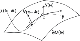
Figure 11: The inverse trajectory of $x$ intersects $M^{o}(t_{0})$.

Theorem 39

For $p=(u_{0},v_{0},t_{0})\in{\cal F}$,

$$\theta(p)=\ddot{\lambda}(t_{0})=\left<-\ddot{\sigma}+2\dot{A}\cdot V,N\right>+\kappa v^{2}$$

where $\kappa$ is the normal curvature of $S$ at $(u_{0},v_{0})$ along velocity $V(p)$, $N$ is the unit outward normal to $S$ at $(u_{0},v_{0})$ and $v^{2}=\left<V(p),V(p)\right>$.

See Appendix for the proof.

From Theorem 39 it is clear that the function $\theta$ is intimately connected with the curvature of the solid and that of the trajectory. It is easy to see that the function $\lambda$ is identical to the function $\varphi$ defined in [4] for implicitly defined solids, albeit, is invariant of the function defining the solid as well as the parametrization of the same.

5.6 Proof of Theorem 33

Proof. Suppose that for all $p\in{\cal F}$, $\theta(p)>0$. For $p\in{\cal F}$, let $t(p)$ denote the $t$-coordinate of $p$. Consider the set of points $P=\left\{p\in{\cal F}|\exists p^{\prime}\in{\cal F},p^{\prime}\neq p,\sigma(p)=\sigma(p^{\prime})\right.$ and $\left.\sigma^{-1}(\sigma(p))=\{p,p^{\prime}\}\right\}$. By the general position assumption, $P$ is a collection of smooth curves in ${\cal F}$. For $p\in P$, let $p^{\prime}$ denote the unique point in $P$ such that $p\neq p^{\prime}$ and $\sigma(p)=\sigma(p^{\prime})$. Further, we define $\delta(p)=\|t(p)-t(p^{\prime})\|$. Let $\delta:=\displaystyle\inf_{p\in P}\delta(p)$. Consider two cases as follows:

Case (i): $\delta=0$, i.e., there exists a sequence $(p_{n})$ in a curve $C$ of $P$ such that $\displaystyle\lim_{n\to\infty}\delta(p_{n})=0$. Hence there exists $p_{0}\in\bar{C}$ (closure of $C$) which is a limit point of $(p_{n})$. Since $\displaystyle\lim_{n\to\infty}\delta(p_{n})=\displaystyle\lim_{n\to\infty}\|t(p_{n})-t(p^{\prime}_{n})\|=0$ and $\partial M$ is free from self-intersections, we have that $\displaystyle\lim_{n\to\infty}\|p_{n}-p^{\prime}_{n}\|=0$. Hence, for a small neighborhood ${\cal N}$ of $p_{0}$ in ${\cal F}$, we may parametrize the smooth curve $\bar{C}\cap{\cal N}$ by a map $\gamma$ so that $\gamma(0)=p_{0}$ and, for $s\neq 0$, $\gamma(s),\gamma(-s)\in C\cap{\cal N}$ and $\sigma(\gamma(s))=\sigma(\gamma(-s))$. Let $\Gamma(s):=\sigma(\gamma(s))$. Note that $\Gamma(s)=\Gamma(-s)$. Now,

$$\frac{d\Gamma}{ds}|_{0}= \displaystyle\lim_{\Delta s\to 0}\frac{\Gamma(\Delta s)-\Gamma(0)}{\Delta s}=\lim_{\Delta s\to 0}\frac{\Gamma(0)-\Gamma(-\Delta s)}{\Delta s}$$

$$= \lim_{\Delta s\to 0}\frac{\Gamma(0)-\Gamma(\Delta s)}{\Delta s}=\displaystyle-\lim_{\Delta s\to 0}\frac{\Gamma(\Delta s)-\Gamma(0)}{\Delta s}$$

Hence,

$$\frac{d\Gamma}{ds}\arrowvert_{0}=J_{\sigma}|_{\gamma(0)}.\frac{d\gamma}{ds}|_{0}=0$$

Since $\frac{d\gamma}{ds}|_{0}\in\mathcal{T}_{\mathcal{F}}(p_{0})$, the map $\sigma|_{{\cal F}}:{\cal F}\to C_{I}$ fails to be an immersion at $p_{0}$ and by Lemma 37 we get that $\theta(p_{0})=0$, which is a contradiction to the hypothesis.

Case (ii): $\delta>0$. Let $\{I_{1},I_{2},\ldots,I_{k}\}$ be a partition of $I$ of width $\frac{\delta}{2}$. Let ${\cal F}_{i}$ and ${\cal C}_{I_{i}}$ denote the funnel and the contact set corresponding to subinterval $I_{i}$. Then it is clear that for each $i$, $\sigma:{\cal F}_{i}\to{\cal C}_{I_{i}}$ is a diffeomorphism, i.e., for each $i$, ${\cal C}_{I_{i}}(t)\cap{\cal C}_{I_{i}}(t^{\prime})=\emptyset$ for all $t,t^{\prime}\in I_{i}$, $t\neq t^{\prime}$. We show that the subproblems $(M,h,I_{i})$ are simple for all $i$. Suppose not, i.e., for some $i$, there exists $t\in I_{i}$ such that $C_{I_{i}}(t)\cap M^{o}(t^{\prime})\neq\emptyset$ for some $t^{\prime}\in I_{i}$. Hence the trim set $T_{I_{i}}$ is not empty. By Lemma 29, for all but finitely many points in $\partial T_{I_{i}}$ there are two points $p_{1},p_{2}\in\partial pT_{I_{i}}$ such that $\sigma(p_{1})=\sigma(p_{2})=y$. If $p_{1}\in{\cal F}_{i}(t_{1})$ and $p_{2}\in{\cal F}_{i}(t_{2})$ then it follows that $C_{I_{i}}(t_{1})\cap C_{I_{i}}(t_{2})=y$ leading to contradiction. Hence, the subproblems $(M,h,I_{i})$ are simple for all $i$. It follows that $(M,h,I)$ is decomposable with width-parameter $\frac{\delta}{2}$.

Hence we have proved that if for all $p\in{\cal F}$, $\theta(p)>0$ then the sweep is decomposable.

Suppose now that there exists $p=(u,v,t)\in{\cal F}$ such that $\theta(p)<0$. Let $y=\sigma(p)$. Recall the definition of the function $\lambda$ from Equation 15 and relation $\theta(p)=\ddot{\lambda}(t)$ from Theorem 39. Clearly, if $\ddot{\lambda}(t)<0$, then $t$ is a local maxima of the function $\lambda$ and the inverse trajectory of $y$ intersects $M^{o}(t)$. So, there exists $\epsilon>0$ such that for all $\delta\in(0,\epsilon)$, there exists $w_{\delta}\in M^{o}(t)$ such that $A(t+\delta)\cdot w_{\delta}+b(t+\delta)=y$. Hence, the interval $[t,t+\delta]\subset L(p)$. Thus $\ell(p)=0$ and hence $,=0$. By Proposition 31, the sweep is non-decomposable. $\square$

6 Trimming non-decomposable sweeps

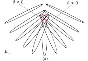
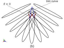
Figure 12: Example of a non-decomposable sweep: a sphere being swept along a parabola (a) Curves of contact at a few time instances (b) The curve $\theta=0$ is shown in red and trim curve is shown in blue.

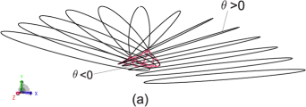
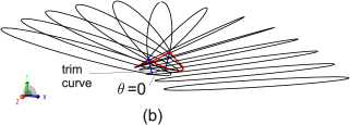
Figure 13: Example of a non-decomposable sweep: an ellipsoid being swept along a circular arc (a) Curves of contact at a few time instances (b) The curve $\theta=0$ is shown in red and trim curve is shown in blue.

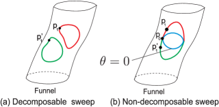
Figure 14: The p-trim curves for decomposable and non-decomposable sweeps shown on ${\cal F}$. Here, $\sigma(p_{1})=\sigma(p_{1}^{\prime})$. The point $p_{0}$ is a singular trim point.

We recall from Section 3, the classification of the curves of $\partial pT_{I}$ as being elementary or singular. In this section we look at singular p-trim curves, i.e., a curve $C$ of $\partial pT_{I}$ where $\displaystyle\inf_{p\in C}\ell(p)=0$. Figure 14(b) schematically illustrates singular p-trim curves. Figures 12 and 13 show two examples of non-decomposable sweeps and the associated singular trim curves. In Figure 12 a sphere undergoes curvilinear motion along a parabola and in Figure 13 an ellipsoid undergoes curvilinear motion along a circular arc. In Figures 12(a) and 13(a), curves of contact at a few time instances are shown. The portions of $C_{I}(t)$ where $\theta>0$ and $\theta<0$ on ${\cal F}(t)$ are shown in black and pink respectively. By Proposition 42, the points where $\theta$ is negative do not lie on ${\cal E}$. In Figures 12(b) and 13(b) such points are excised, the curve ${C_{I}}^{0}$ is shown in red and the trim curve $\partial T_{I}$ is shown in blue. Note that ${C_{I}}^{0}$ and $\partial T_{I}$ make contact, which they must, as we explain in this section. Figure 15 schematically illustrates the interaction between curves of contact in non-decomposable sweeps.

Proposition 40

If $C$ is a singular p-trim curve and $p_{0}\in C$ is a limit-point of $(p_{n})\subset C$ such that $\displaystyle\lim_{n\to\infty}\ell(p_{n})=0$, then $\theta(p_{0})=0$.

Proof. The proof is similar to Case (i) of proof for Theorem 33.

Definition 41

A limit point $p$ of a singular p-trim curve $C$ such that $\theta(p)=0$ will be called a singular trim point.

In Figure 14(b) a singular trim point $p_{0}$ is shown on $\partial pT_{I}$.

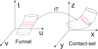
Figure 15: A schematic illustrating the interaction between curves of contact in non-decomposable sweeps.

Proposition 42

If $p_{0}\in{\cal F}$ such that $\theta(p_{0})<0$ then $p_{0}\in pT_{I}$.

Proof. Let $p_{0}=(u_{0},v_{0},t_{0})\in{\cal F}$. Recall the definition of the function $\lambda$ from Equation 15 and relation $\theta(p_{0})=\ddot{\lambda}(t_{0})$ from Theorem 39. Clearly, if $\ddot{\lambda}(t_{0})<0$, then $t_{0}$ is a local maxima of the function $\lambda$ and the inverse trajectory of $\sigma(p_{0})$ intersects $M^{o}(t_{0})$ and $\sigma(p_{0})\in T_{I}$. Hence, if $\theta(p_{0})<0$ then $p_{0}\in pT_{I}$. $\square$

The above two propositions link the curves of ${\cal F}^{0}$ to the curves of $\partial pT_{I}$. We see that every curve of ${\cal F}^{0}$ lies inside a curve of $\partial pT_{I}$ and every curve $C$ of $\partial pT_{I}$ has a curve ${\cal F}^{0}_{C}$ of ${\cal F}^{0}$ which makes contact with it. We have already seen that ${\cal F}^{0}$ is a collection of curves on which $\nabla\theta$ is non-zero. Thus, the computation of ${\cal F}^{0}$ in modern kernels is straightforward. The task before us is now to locate the points of ${\cal F}^{0}\cap\partial pT_{I}$. This is enabled by the following function.

Definition 43

Let $\Omega$ be a parametrization of a curve ${\cal F}^{0}_{i}$ of ${\cal F}^{0}$. Let $\Omega(s_{0})=p_{0}\in{\cal F}^{0}_{i}$ and $\bar{z}:=(l,m,-1)\in null(J_{\sigma})$ at $p_{0}$, i.e., $l\sigma_{u}+m\sigma_{v}=\sigma_{t}$. Define the function $\varphi:{\cal F}^{0}\to\mathbb{R}$ as follows.

$$\varphi(s_{0})=\left<\bar{z}\times\frac{d\Omega}{ds}|_{s_{0}},\nabla f|_{p_{0}}\right>$$ (7)

where $\times$ is the cross-product in $\mathbb{R}^{3}$.

Here, $\varphi$ is a measure of the oriented angle between the tangent at $p_{0}$ to ${\cal F}^{0}_{i}$ and the kernel (line) of the Jacobian $J_{\sigma}$ restricted to the tangent space ${\cal T}_{\cal F}(p_{0})$.

Proposition 44

Every singular p-trim curve $C$ makes contact with a curve ${\cal F}^{0}_{i}$ of ${\cal F}^{0}$ so that if $p_{0}$ is a singular trim point of $C$ then $\varphi(p_{0})=0$. Furthermore, at such points, $\varphi^{\prime}(p_{0})\neq 0$ where $\varphi^{\prime}$ refers to the derivative of $\varphi$ along the curve ${\cal F}^{0}_{i}$.

Proof. We know from Proposition 42 that ${\cal F}^{-}\subset pT_{I}$. Since ${\cal F}^{0}$ and $\partial pT_{I}$ form the boundaries of ${\cal F}^{-}$ and $pT_{I}$ respectively, ${\cal F}^{0}$ and a singular p-trim curve $C$ of $\partial pT_{I}$ meet tangentially at the singular trim point. Further, by an argument similar to the case (i) of Theorem 33, it can be seen that at a singular trim point $p_{0}$, ${\cal T}_{C}(p_{0})$ is the null-space of the Jacobian $J_{\sigma}|_{p_{0}}$. Since ${\cal T}_{C}(p_{0})={\cal T}_{{\cal F}^{0}}(p_{0})$, $J_{\sigma}|_{p_{0}}({\cal T}_{{\cal F}^{0}}(p_{0}))=0$. Since the function $\varphi$ measures the oriented angle between $null(J_{\sigma})$ and ${\cal T}_{{\cal F}^{0}}$, it follows that $\varphi(p_{0})=0$.

The derivative $\varphi^{\prime}\neq 0$ at singular trim points for non-decomposable sweeps shown in Figure 12 and Figure 13. $\square$

Proposition 44 confirms that for every singular p-trim curve, we may use the function $\varphi$ to locate a singular trim point $p_{0}$ in a computationally robust manner. Thus, via $\theta$ and $\varphi$ we may access every component of $\partial pT_{I}$.

Proposition 45

In the generic situation, (i) the singular p-trim curve $C$ has a finite set of singular trim points. Each of these points lie on a curve of ${\cal F}^{0}$. (ii) For all but finitely many non-singular points $p\in C$, the image $\sigma(p)$ lies on the transversal intersection of two surface patches $\sigma({\cal F}_{i})$ and the remaining non-singular points lie on intersection of three surface patches $\sigma({\cal F}_{i})$ where each ${\cal F}_{i}\subset{\cal F}$ corresponds to a suitable subinterval $I_{i}\subset I$.

Proof. It follows from Proposition 40 that the singular trim points lie on ${\cal F}^{0}$. Since at a non-singular trim point $p\in C$, $\ell(p)>0$, the proof for (ii) is identical to the proof for Lemma 29 about elementary trim curves. $\square$

Note that the computation of $C$ above is transversal except at the known point $p_{0}\in{\cal F}^{0}$, i.e., where $\varphi=0$. The problem then reduces to a surface-surface intersection which is transversal except at a known point. This information is usually enough for most kernels to compute $C$ robustly.

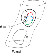
Figure 16: A singular p-trim curve nested inside an elementary p-trim curve

Figure 16 schematically illustrates a scenario in which a singular p-trim curve is nested inside an elementary p-trim curve. Note that the sweep is non-decomposable and this will be detected by the presence of points on ${\cal F}$ where $\theta$ is negative. Further, the region bounded by the singular p-trim curve needs to be excised before a surface-surface intersection algorithm can trace the elementary trim curves since no neighborhood of $C_{I}^{0}$ (where $\theta$ is zero) can be parametrized. Our analysis will first successfully identify and excise the region bound by the singular p-trim curve. After parametrizing the remaining part, the task of excising the regions bound by elementary p-trim curves can be handled by existing kernels.

7 Discussion

This paper develops a mathematical framework for the implementation of the “generic” solid sweep in modern solid modelling kernels. This is done via a complete understanding of singularities and of self-intersections within the envelope and the notion of decomposability. This in turn is done through the important invariant $\theta$ by which all trim-curves are either stable surface-surface intersections or are caught by $\theta$.

We now detail certain implementation issues. Firstly, the use of funnel as the parametrization space and the so called “procedural” framework is now standard, see e.g., the ACIS kernel. Secondly, the non-generic case in the sweep, as in blends or surface-surface intersections, will need careful programming and convergence with existing kernel methods for handling degeneracy. Next, while we have not tackled the case when the trim curves intersect the left/right caps, that analysis is not difficult and we skip it for want of space. Finally, the non-smooth sweep is a step away. The local geometry is already available. The trim curves and other combinatorial/topological properties of the smooth and non-smooth case are tackled in a later paper.

Mathematically, our framework may also extend to more complicated cases where the curves of contact are not simple. This calls for a more Morse-theoretic analysis which should yield rich structural insights. The invariant $\theta$ is surprisingly strong and needs to be studied further.

Appendix A Application of solid sweep in design of conveyor screws

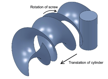
Figure 17: A conveyor screw for translating cylindrical bottles.

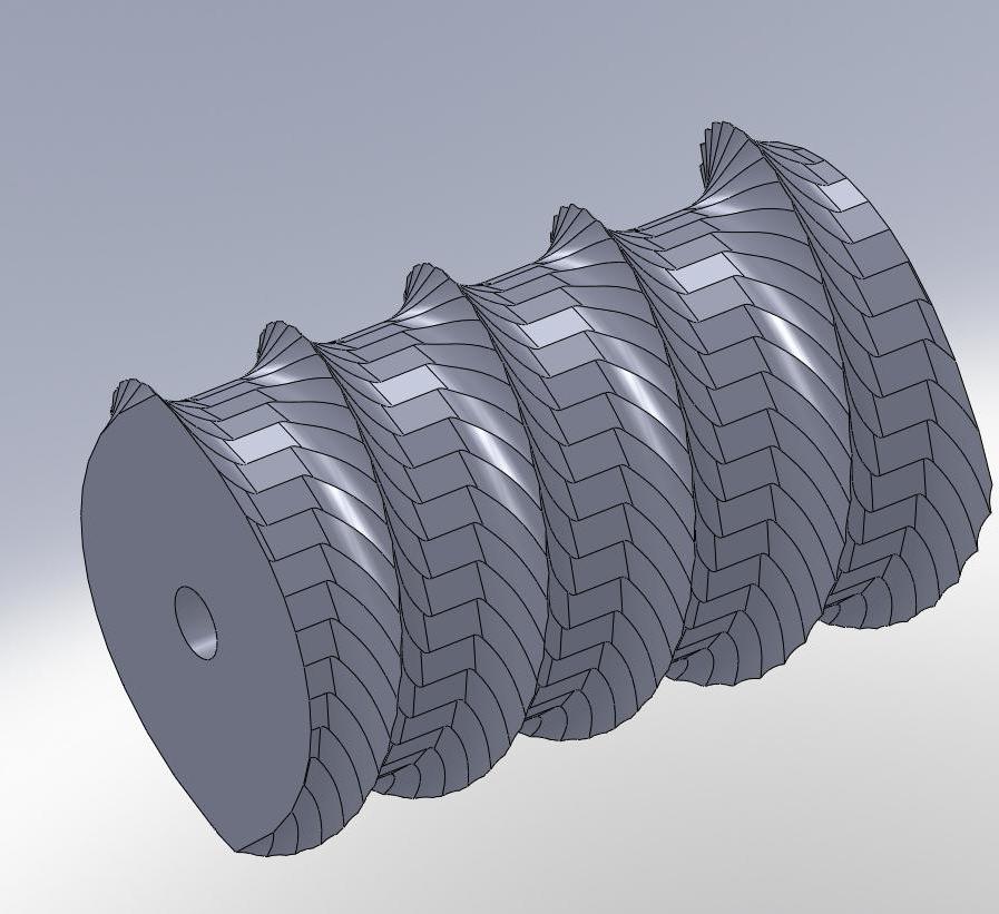
Figure 18: A conveyor screw designed via discrete approach using boolean operations.

In this section we briefly describe an application of solid sweep in the packaging industry where complex needs for handling products arise. A few example scenarios are, orienting the products precisely as they pass along the assembly line, separating one stream of products into two streams or combing two streams into one, inverting the product as it passes along the line, introducing exact spacing between consecutive products, and so on. This is often achieved by a conveyor screw which rotates about its own axis and hence propels the product ahead which is sitting in its groove. The surface of this screw is specifically designed for moving the required product along the required path. See [15] for a video of conveyor screws which group a set of products together and introduce precise time lag between two consecutive products.

In order to design such a screw for the required object and the required motion profile, the rotation of the screw is compounded into the desired motion profile. The object is then swept along the resultant trajectory and the swept volume so obtained is subtracted from a cylinder to obtain the conveyor screw. Figure 17 shows the surface of a screw designed to translate a cylinder. The conventional method of designing such screws involves sampling the trajectory at a finite number of positions, and taking the union of the object positioned at all these positions. The resultant “discrete” swept volume is then subtracted from the cylinder to obtain an approximate screw. This is shown in Figure 18. As expected, this approach produces a large number of sliver faces and the brep structure of the resulting solid has a high degree of complexity. Further, the solution is neither accurate nor smooth.

Appendix B Proof for Proposition 8

Recall the statement of Proposition 8 that for $(y,x,t)\in R$ and $I=[t_{0},t_{1}]$, either (i) $t=t_{0}$ and $g(x,t)\leq 0$, or (ii) $t=t_{1}$ and $g(x,t)\geq 0$ or (iii) $g(x,t)=0$.

Proof. Define $\hat{e}_{1},\hat{e}_{2},\hat{e}_{3}$ and $\hat{e}_{4}$ as $(1,0,0,0),(0,1,0,0),$ $(0,0,1,0)$ and $(0,0,0,1)$ respectively. We define the following objects in $\mathbb{R}^{4}$ where the fourth dimension is time. Let $Z:=\{(A(t)\cdot x+b(t),t)|\mbox{ where }x\in M\mbox{ and }t\in I\}$ and $X:=\{(A(t)\cdot x+b(t),t)|\mbox{ where }x\in\partial M\mbox{ and }t\in I\}$. Note that $Z$ is a four dimensional topological manifold and $X$ is a three dimensional submanifold of $Z$. Further, a point $(x,t)$ lies in $Z^{o}$ if $t\in I^{o}$ and $x\in M^{o}(t)$. Further, if $I=[t_{0},t_{1}]$, $\partial Z=X\cup(M(t_{0}),t_{0})\cup(M(t_{1}),t_{1})$ forms the boundary of $Z$ where Define the projection $\mu:\mathbb{R}^{3}\times I\to\mathbb{R}^{3}$ is defined as $\mu(x,t)=x$ and the projection $\tau:\mathbb{R}^{3}\times I\to\mathbb{R}$ is defined as $\tau(x,t)=t$. Clearly, for a point $w\in\mu(Z)$, if $\mu^{-1}(w)\cap Z^{o}\neq\emptyset$ then $w\notin{\cal E}$. Hence a necessary condition for $w$ to be in ${\cal E}$ is that the line $\mu^{-1}(w)$ should be tangent to $\partial Z$ which is a three dimensional manifold which is smooth everywhere except at $(\partial M(t_{0}),t_{0})$ and at $(\partial M(t_{1}),t_{1})$. For $w\in M^{o}(t_{0})$, the outward normal to $\partial Z$ at $(w,t_{0})$ is given by $-\hat{e}_{4}$ and the outward normal to $\partial Z$ at $(w,t_{1})\in(M^{0}(t_{1}),t_{1})$ is given by $\hat{e}_{4}$. We now compute the outward normal to $\partial Z$ at $(w,t)\in X$. The manifold $X$ is diffeomorphic to $\partial M\times I$, i.e., the cross product of $\partial M$ which is a 2-dimensional manifold and $I$ which is a 1-dimensional manifold, with the diffeomorphism given by $d:\partial M\times I\to X$, $d(x,t)=(A(t)\cdot x+b(t),t)$. Hence, if $\{y_{1},y_{2}\}$ spans ${\cal T}_{\partial M}(x)$ and $\{1\}$ spans ${\cal T}_{\mathbb{R}}(t)$ then the tangent space of $\partial M\times I$ at $(x,t)$ is spanned by $\{(y_{1},0),(y_{2},0),\hat{e}_{4}\}$ and ${\cal T}_{X}(w,t)$ is spanned by
$\left\{(A(t)\cdot y_{1},0),(A(t)\cdot y_{2},0),(A^{\prime}(t)\cdot x+b^{\prime}(t),1)\right\}$. Hence, the outward normal to $\partial Z$ at $(w,t)$ is $(A(t)\cdot N(x),\\ -\left<A(t)\cdot N(x),v_{x}(t)\right>)$. Consider now three cases as follows.

Case (i): $t=t_{0}$. At any point $(w,t_{0})\in(\partial M(t_{0}),t_{0})$ there is a cone of outward normals given by $\alpha\begin{bmatrix}A(t)\cdot N(x)\\ -\left<A(t)\cdot N(x),v_{x}(t)\right>\end{bmatrix}-\beta\hat{e}_{4}$ where $\alpha,\beta\in\mathbb{R}$ and $\alpha,\beta\geq 0$. So if the line $\mu^{-1}(w)$ is tangent to $\partial Z$ at $(w,t_{0})$ then

$$\left<\hat{e}_{4},\alpha\begin{bmatrix}A(t)\cdot N(x)\\ -\left<A(t)\cdot N(x),v_{x}(t)\right>\end{bmatrix}-\beta\hat{e}_{4}\right>=0$$

for some $\alpha,\beta$ where $\alpha>0$ and $\beta\geq 0$. Solving the above for $\left<A(t)\cdot N(x),v_{x}(t)\right>$ we get $\left<A(t)\cdot N(x),v_{x}(t)\right>=-\frac{\beta}{\alpha}\leq 0$. Hence $g(x,t)\leq 0$.

Case (ii): $t=t_{1}$. Proof is similar to case (i).

Case (iii): $t\in I^{o}$. If the line $\mu^{-1}(w)$ is tangent to $X$ at $(w,t)$ there exist $a,b,c\in\mathbb{R}$ not all zero such that

$$a\begin{bmatrix}A(t)\cdot y_{1}\\ 0\end{bmatrix}+b\begin{bmatrix}A(t)\cdot y_{2}\\ 0\end{bmatrix}+c\begin{bmatrix}A^{\prime}(t)\cdot x+b^{\prime}(t)\\ 1\end{bmatrix}=\hat{e}_{4}$$

It follows that $v_{x}(t)=A^{\prime}(t)\cdot x+b^{\prime}(t)\in span\{A(t)\cdot y_{1},A(t)\cdot y_{2}\}={\cal T}_{\partial M(t)}(x)$. In other words, $\left<A(t)\cdot N(x),v_{x}(t)\right>=g(x,t)=0$. $\square$

Appendix C Some useful facts about the inverse trajectory

Recall the inverse trajectory of a fixed point $x$ as $\bar{y}(t)=A^{t}(t)\cdot(x-b(t))$. We will denote the trajectory of $x$ by $y:[0,1]\to\mathbb{R}^{3}$, $y(t)=A(t)\cdot x+b(t)$. We now note a few useful facts about $\bar{y}$. We assume without loss of generality that $A(t_{0})=I$ and $b(t_{0})=0$. Denoting the derivative with respect to $t$ by $\dot{}$, we have

$$\dot{\bar{y}}(t)=\dot{A}^{t}(t)\cdot(x-b(t))-A^{t}(t)\cdot\dot{b}(t)$$ (8)

Since $A\in SO(3)$ we have,

$$A^{t}(t)\cdot A(t) =I,\forall t$$ (9)

Differentiating Eq. 9 w.r.t. $t$ we get

$$\dot{A}^{t}(t_{0})+\dot{A}(t_{0}) =0$$ (10)

$$\ddot{A}^{t}(t_{0})+2\dot{A}^{t}(t_{0})\cdot\dot{A}(t_{0})+\ddot{A}(t_{0}) =0$$ (11)

Using Eq. 8 and Eq. 10 we get

$$\dot{\bar{y}}(t_{0}) =-\dot{A}(t_{0})\cdot x-\dot{b}(t_{0})=-\dot{y}(t_{0})$$ (12)

Differentiating Eq. 8 w.r.t. time we get

$$\ddot{\bar{y}}(t)=\ddot{A}^{t}(t)\cdot(x-b(t))-2\dot{A}^{t}(t)\cdot\dot{b}(t)-A^{t}(t)\cdot\ddot{b}(t)$$ (13)

Using Equations 13, 10 and 11 we get

$$\ddot{\bar{y}}(t_{0})=-\ddot{y}(t_{0})+2\dot{A}(t_{0})\cdot\dot{y}(t_{0})$$ (14)

Appendix D Proof of Theorem 39

Proof. Recall the definition of function $\lambda$ as

$$\lambda(t)=\left<\bar{y}(t)-\pi(t),N(t)\right>$$ (15)

Differentiating Eq. 15 with respect to time and denoting derivative w.r.t. $t$ by $\dot{}$, we get

$$\dot{\lambda}(t) =\left<\dot{\bar{y}}(t)-\dot{\pi}(t),N(t)\right>+\left<\bar{y}(t)-\pi(t),\dot{N}(t)\right>$$ (16)

$$\ddot{\lambda}(t) =\left<\ddot{\bar{y}}(t)-\ddot{\pi}(t),N(t)\right>+2\left<\dot{\bar{y}}(t)-\dot{\pi}(t),\dot{N}(t)\right>$$

$$+\left<\bar{y}(t)-\pi(t),\ddot{N}(t)\right>$$ (17)

At $t=t_{0}$, $\bar{y}(t_{0})=\pi(t_{0})$. Since $\dot{y}(t_{0})=V(p)\bot N(p)$, it follows from Eq. 12 that $\dot{\bar{y}}(t_{0})\bot N(p)$. It is easy to verify that $\dot{\pi}(t_{0})=\dot{\bar{y}}(t_{0})$. Hence,

$$\lambda(t_{0})=\dot{\lambda}(t_{0})=0$$ (18)

From Eq. 17 and Eq. 14 it follows that

$$\ddot{\lambda}(t_{0}) =\left<\ddot{\bar{y}}(t_{0})-\ddot{\pi}(t_{0}),N(t_{0})\right>$$

$$=\left<-\ddot{y}(t_{0})+2\dot{A}(t_{0})\cdot\dot{y}(t_{0})-\ddot{\pi}(t_{0}),N(t_{0})\right>$$ (19)

Since $\pi(t)\in S(t_{0})$ for all $t$ in some neighbourhood $U$ of $t_{0}$, we have that $\left<\dot{\pi}(t),N(t)\right>=0,\forall t\in U$. Hence $\left<\ddot{\pi}(t),N(t)\right>+\left<\dot{\pi}(t),\dot{N}(t)\right>=0,\forall t\in U$. Hence $-\left<\ddot{\pi}(t_{0}),N(t_{0})\right>=\left<\dot{\pi}(t_{0}),\dot{N}(t_{0})\right>=\left<\dot{\pi}(t_{0}),\mathcal{G}^{*}(\dot{\pi}(t_{0}))\right>=\left<\dot{y}(t_{0}),\mathcal{G}^{*}(\dot{y}(t_{0}))\right>$ = $\left<V(p),\mathcal{G}^{*}(V(p))\right>=\kappa v^{2}$. Here $\mathcal{G}^{*}$ is the differential of the Gauss map, i.e. the curvature tensor of $S(t_{0})$ at point $x$. Using this in Eq. 19 and the fact that $\dot{y}(t_{0})=\dot{\sigma}(p)$, $\ddot{y}(t_{0})=\ddot{\sigma}(p)$ we get

$$\ddot{\lambda}(t_{0}) =\left<-\ddot{\sigma}(p)+2\dot{A}(t_{0})\cdot V(p),N(t_{0})\right>+\kappa v^{2}$$ (20)

Recalling that $\theta(p)=lf_{u}+mf_{v}-f_{t}$

$$lf_{u}+mf_{v}-f_{t} =\left<l\hat{N}_{u}+m\hat{N}_{v},V\right>+\left<\hat{N},lV_{u}+mV_{v}\right>$$

$$-\left<\hat{N}_{t},V\right>-\left<\hat{N},V_{t}\right>$$

Here $\hat{N}_{u}=\mathcal{G}^{*}(\sigma_{u})$ and $\hat{N}_{v}=\mathcal{G}^{*}(\sigma_{v})$ where $\mathcal{G}^{*}$ is the shape operator (differential of the Gauss map) of $S(t_{0})$ at $(u_{0},v_{0})$. Also, $V_{u}=A_{t}\cdot S_{u}$ and $V_{v}=A_{t}\cdot S_{v}$. Assume without loss of generality that $A(t_{0})=I$ and $b(t_{0})=0$, hence $\hat{N}=A(t_{0})\cdot N=N$, $\sigma_{u}=S_{u}$ and $\sigma_{v}=S_{v}$. Using Eq. 10 and the fact that $V=\sigma_{t}=l\sigma_{u}+m\sigma_{v}$ we get

$$lf_{u}+mf_{v}-f_{t} =\left<\mathcal{G}^{*}\cdot V,V\right>+2\left<A_{t}\cdot V,N\right>-\left<V_{t},N\right>$$

$$=\kappa v^{2}+\left<2A_{t}\cdot V-V_{t},N\right>$$ (21)

From Eqs. 20 and 21 and the fact that $\frac{\partial\sigma}{\partial t^{2}}=V_{t}$ we get $\theta(p)=lf_{u}+mf_{v}-f_{t}=\ddot{\lambda}(t_{0})$. $\square$

Appendix E Procedural parametrization of the simple sweep

We now describe the parametrization of $E:=C_{I}$ assuming that the sweep $(M,h,I)$ is simple. We obtain a procedural parametrization of $E$ which is an abstract way of defining curves and surfaces. This approach relies on the fact that from the user’s point of view, a parametric surface(curve) in $\mathbb{R}^{3}$ is a map from $\mathbb{R}^{2}$($\mathbb{R}$) to $\mathbb{R}^{3}$ and hence is merely a set of programs which allow the user to query the key attributes of the surface(curve), e.g. its domain and to evaluate the surface(curve) and its derivatives at the given parameter value. This approach to defining geometry is especially useful when closed form formulae are not available for the parametrization map and one must resort to iterative numerical methods. We use the Newton-Raphson(NR) method for this purpose. As an example, the parametrization of the intersection curve of two surfaces is computed procedurally in [9]. This approach has the advantage of being computationally efficient as well as accurate. For a detailed discussion on the procedural framework, see [10].

The computational framework is as follows. Given $S$ and $h$, an approximate funnel is first computed, which we will refer to as the seed surface. Now, when the user wishes to evaluate $E$ or its derivative at some parameter value, a NR method will be started with seed obtained from the seed surface. The NR method will converge, upto the required tolerance, to the required point on $E$, or to its derivative, as required. Here, the precision of the evaluation is only restricted by the finite precision of the computer and hence is accurate. It has the advantage that if a tighter degree of tolerance is required while evaluation of the surface or its derivative, the seed surface does not need to be recomputed. Thus, for the procedural definition of $E$ we need the following:

1. an NR formulation for computing points on ${E}$ and its derivatives, which we describe in Section E.1

2. Seed surface for seeding the NR procedure, which we describe in Section E.2

Recall that by the non-degeneracy assumption, ${E}$ is the union of $E(t):=C_{I}(t),\forall t$. This suggests a natural parametrization of ${E}$ in which one of the surface parameters is time $t$. We will call the other parameter $p$ and denote the seed surface by $\gamma$ which is a map from the parameter space of ${E}$ to the parameter space of $\mathcal{\sigma}$, i.e. $\gamma(p,t)=(\bar{u}(p,t),\bar{v}(p,t),t)$ and while the point $\sigma(\gamma(p,t))$ may not belong to ${E}$, it is close to ${E}$. In other words, $\gamma(p,t)$ is close to $\mathcal{F}$. We call the image of the seed surface through the sweep map $\sigma$ as the approximate envelope and denote it by $\bar{{E}}$, i.e. $\bar{{E}}(p,t)=\sigma(\gamma(p,t))$. We make the following assumption about $\bar{{E}}$.

Assumption 46

At every point on the iso-t curve of $\bar{{E}}$, the normal plane to the iso-t curve intersects the iso-t curve of ${E}$ in exactly one point.

Note that this is not a very strong assumption and holds true in practice even with rather sparse sampling of points for the seed surface. We now describe the Newton-Raphson formulation for evaluating points on ${E}$ and its derivatives at a given parameter value.

E.1 NR formulation for ${E}$

Recall that the points on ${E}$ were characterized by the tangency condition $f(u,v,t)=0$. Introducing the parameters $(p,t)$ of ${E}$, we rewrite this equation $\forall(p_{0},t_{0})$:

$$f(u(p_{0},t_{0}),v(p_{0},t_{0}),t_{0}) =\left<\hat{N}(u(p_{0},t_{0}),v(p_{0},t_{0}),t_{0}),\right.$$

$$\left.V(u(p_{0},t_{0}),v(p_{0},t_{0}),t_{0})\right>=0$$ (22)

So, given $(p_{0},t_{0})$, we have one equation in two unknowns, viz. $u(p_{0},t_{0})$ and $v(p_{0},t_{0})$. ${E}(p_{0},t_{0})$ is defined as the intersection of the plane normal to the iso-$t$(for $t=t_{0}$) curve of $\bar{{E}}$ at $\bar{{E}}(p_{0},t_{0})$ with the iso-$t$(for $t=t_{0}$) curve of ${E}$ which is nothing but $C_{I}(t_{0})$. Recall that $C_{I}(t_{0})$ is given by $\sigma(u(p,t_{0}),v(p,t_{0}),t_{0})$ where $u,v,t_{0}$ obey Eq. E.1. Henceforth, we will suppress the notation that $u,v,\bar{u}$ and $\bar{v}$ are functions of $p$ and $t$. Also, all the evaluations will be understood to be done at parameter values $(p_{0},t_{0})$. The tangent to iso-$t$ curve of $\bar{{E}}$ at $(p_{0},t_{0})$ is given by

$$\frac{\partial\bar{{E}}}{\partial p}=\frac{\partial\sigma}{\partial u}\frac{\partial\bar{u}}{\partial p}+\frac{\partial\sigma}{\partial v}\frac{\partial\bar{v}}{\partial p}$$ (23)

Hence, ${E}(p_{0},t_{0})$ is the solution of simultaneous system of equations E.1 and 24

$$\left<\sigma(u,v,t_{0})-\sigma(\bar{u},\bar{v},t_{0}),\frac{\partial\bar{{E}}}{\partial p}\right>=0$$ (24)

Eq. E.1 and Eq. 24 give us a system of two equations in two unknowns, $u$ and $v$ and hence can be put into NR framework by computing their first order derivatives w.r.t $u$ and $v$. For any given parameter value $(p_{0},t_{0})$, we seed the NR method with the point $(\bar{u}(p_{0},t_{0}),\bar{v}(p_{0},t_{0}))$ and solve Eq. E.1 and Eq. 24 for $(u(p_{0},t_{0}),v(p_{0},t_{0}))$ and compute ${E}(p_{0},t_{0})$.

Having computed ${E}(p,t)$ we now compute first order derivatives of ${E}$ assuming that they exist. In order to compute $\frac{\partial{E}}{\partial p}$, we differentiate Eq. E.1 and Eq. 24 w.r.t. $p$ to obtain

$$\left<\frac{\partial\hat{N}}{\partial u}\frac{\partial u}{\partial p}+\frac{\partial\hat{N}}{\partial v}\frac{\partial v}{\partial p},V\right>+\left<\hat{N},\frac{\partial V}{\partial u}\frac{\partial u}{\partial p}+\frac{\partial V}{\partial v}\frac{\partial v}{\partial p}\right>=0$$ (25)

$$\left<\frac{\partial\sigma}{\partial u}\frac{\partial u}{\partial p}+\frac{\partial\sigma}{\partial v}\frac{\partial v}{\partial p}-\frac{\partial\sigma}{\partial u}\frac{\partial\bar{u}}{\partial p}+\frac{\partial\sigma}{\partial v}\frac{\partial\bar{v}}{\partial p},\frac{\partial\bar{{E}}}{\partial p}\right>$$

$$+\left<\sigma(u,v,t_{0})-\sigma(\bar{u},\bar{v},t_{0}),\frac{\partial^{2}\bar{{E}}}{\partial p^{2}}\right>=0$$ (26)

Eq. 25 and Eq. 26 give a system of two equations in two unknowns, viz., $\frac{\partial u}{\partial p}$ and $\frac{\partial v}{\partial p}$ and can be put into NR framework by computing first order derivatives w.r.t. $\frac{\partial u}{\partial p}$ and $\frac{\partial v}{\partial p}$. Note that Eq. 25 and Eq. 26 also involve $u$ and $v$ whose computation we have already described. After computing $\frac{\partial u}{\partial p}$ and $\frac{\partial v}{\partial p}$, $\frac{\partial{E}}{\partial p}$ can be computed as $\frac{\partial\sigma}{\partial u}\frac{\partial{u}}{\partial p}+\frac{\partial\sigma}{\partial v}\frac{\partial{v}}{\partial p}$. $\frac{\partial{E}}{\partial t}$ can similarly be computed by differentiating Eq. E.1 and Eq. 24 w.r.t. $t$. Higher order derivatives can be computed in a similar manner.

E.2 Computation of seed surface

The seed surface is constructed by sampling a few points on the funnel and fitting a tensor product B-spline surface through these points. For this, we first sample a few time instants, say, ${\cal I}=\{t_{1},t_{2},\ldots,t_{n}\}$ from the time interval of the sweep. For each $t_{i}\in{\cal I}$, we sample a few points on the pcurve of contact ${\cal F}(t_{i})$. For this, we begin with one point $p$ on ${\cal F}(t_{i})$ and compute the tangent to ${\cal F}(t_{i})$ at $p$, call it $z$. Then $p+z$ is used as a seed in Newton-Raphson method to obtain the next point on ${\cal F}(t_{i})$ and this process is repeated.

While we do not know of any structured way of choosing the number of sampled points, in practice even a small number of points suffice to ensure that the Assumption 46 is valid.

References

- [1] Abdel-Malek K, Yeh HJ. Geometric representation of the swept volume using Jacobian rank-deficiency conditions. Computer-Aided Design 1997;29(6):457-468.
-
[2]
ACIS 3D Modeler, SPATIAL,
www.spatial.com/products/3d_acis_modeling - [3] Blackmore D, Leu MC, Wang L. Sweep-envelope differential equation algorithm and its application to NC machining verification. Computer-Aided Design 1997;29(9):629-637.
- [4] Blackmore D, Samulyak R, Leu MC. Trimming swept volumes. Computer-Aided Design 1999;31(3):215-223.
- [5] Elber G. Global error bounds and amelioration of sweep surfaces. Computer-Aided Design 1997;29(6):441-447.
- [6] Guillemin V, Pollack A. Differential Topology. Prentice-Hall, 1974.
- [7] Huseyin Erdim, Horea T. Ilies. Classifying points for sweeping solids. Computer-Aided Design 2008;40(9);987-998
- [8] Huseyin Erdim, Horea T. Ilies. Detecting and quantifying envelope singularities in the plane. Computer-Aided Design 2007;39(10);829-840
- [9] Markot R, Magedson R. Procedural method for evaluating the intersection curves of two parametric surfaces. Computer-Aided Design 1990;23(6);395-404
-
[10]
Milind Sohoni. Computer aided geometric design course notes.
www.cse.iitb.ac.in/~sohoni/336/main.ps - [11] Peternell M, Pottmann H, Steiner T, Zhao H. Swept volumes. Computer-Aided Design and Applications 2005;2;599-608
- [12] Seok Won Lee, Andreas Nestler. Complete swept volume generation, Part I: Swept volume of a piecewise C1-continuous cutter at five-axis milling via Gauss map. Computer-Aided Design 2011;43(4);427-441
- [13] Seok Won Lee, Andreas Nestler. Complete swept volume generation, Part II: NC simulation of self-penetration via comprehensive analysis of envelope profiles. Computer-Aided Design 2011;43(4);442-456
- [14] Xu Z-Q, Ye X-Z, Chen Z-Y, Zhang Y, Zhang S-Y. Trimming self-intersections in swept volume solid modelling. Journal of Zhejiang University Science A 2008;9(4):470-480.
-
[15]
Kinsley Inc. Timing screw for grouping and turning.
https://www.youtube.com/watch?v=LooYoMM5DEo