Skew-spectra and skew energy of various products of graphs

Abstract

Given a graph $G$, let $G^{\sigma}$ be an oriented graph of $G$ with the orientation $\sigma$ and skew-adjacency matrix $S(G^{\sigma})$. Then the spectrum of $S(G^{\sigma})$ consisting of all the eigenvalues of $S(G^{\sigma})$ is called the skew-spectrum of $G^{\sigma}$, denoted by $Sp(G^{\sigma})$. The skew energy of the oriented graph $G^{\sigma}$, denoted by $\mathcal{E}_{S}(G^{\sigma})$, is defined as the sum of the norms of all the eigenvalues of $S(G^{\sigma})$. In this paper, we give orientations of the Kronecker product $H\otimes G$ and the strong product $H\ast G$ of $H$ and $G$ where $H$ is a bipartite graph and $G$ is an arbitrary graph. Then we determine the skew-spectra of the resultant oriented graphs. As applications, we construct new families of oriented graphs with maximum skew energy. Moreover, we consider the skew energy of the orientation of the lexicographic product $H[G]$ of a bipartite graph $H$ and a graph $G$.

Keywords: oriented graph, skew-spectrum, skew energy, Kronecker product, strong product, lexicographic product.

AMS Subject Classification 2010: 05C20, 05C50, 05C90

1 Introduction

Let $G$ be a simple undirected graph with vertex set $V(G)=\{v_{1},v_{2},\ldots,v_{n}\}$, and let $G^{\sigma}$ be an oriented graph of $G$ with the orientation $\sigma$, which assigns to each edge of $G$ a direction so that the induced graph $G^{\sigma}$ becomes an oriented graph or a directed graph. Then $G$ is called the underlying graph of $G^{\sigma}$. The skew-adjacency matrix of $G^{\sigma}$ is the $n\times n$ matrix $S(G^{\sigma})=[s_{ij}]$, where $s_{ij}=1$ and $s_{ji}=-1$ if $\langle v_{i},v_{j}\rangle$ is an arc of $G^{\sigma}$, otherwise $s_{ij}=s_{ji}=0$. It is easy to see that $S(G^{\sigma})$ is a skew-symmetric matrix, and thus all its eigenvalues are purely imaginary numbers or 0, which form the spectrum of $S(G^{\sigma})$ and are said to be the skew-spectrum $Sp(G^{\sigma})$ of $G^{\sigma}$.

The concept of the energy of a simple undirected graph was introduced by Gutman in [6]. Then Adiga, Balakrishnan and So in [1] generalized the energy of an undirected graph to the skew energy of an oriented graph. Formally, the skew energy of an oriented graph $G^{\sigma}$ is defined as the sum of the absolute values of all the eigenvalues of $S(G^{\sigma})$, denoted by $\mathcal{E}_{S}(G^{\sigma})$. Most of the results on the skew energy are collected in our recent survey [7], among which the problem about the maximum skew energy has been paid more attention.

In [1], Adiga, Balakrishnan and So derived that for any oriented graph $G^{\sigma}$ with order $n$ and maximum degree $\Delta$, $\mathcal{E}_{S}(G^{\sigma})\leq n\sqrt{\Delta}$. They also showed that the equality holds if and only if $S(G^{\sigma})^{T}S(G^{\sigma})=\Delta I_{n}$, which implies that $G^{\sigma}$ is $\Delta$-regular. Among all oriented graphs with order $n$ and maximum degree $\Delta$, the skew energy $n\sqrt{\Delta}$ is called the maximum skew energy. Naturally, they proposed the following problem:

Problem 1.1

Which $k$-regular graphs on $n$ vertices have orientations $G^{\sigma}$ with $\mathcal{E}_{S}(G^{\sigma})=n\sqrt{k}$, or equivalently, $S(G^{\sigma})^{T}S(G^{\sigma})=kI_{n}$ ?

For $k=1,2,3,4$, all $k$-regular graphs which have orientations $G^{\sigma}$ with $\mathcal{E}_{S}(G^{\sigma})=n\sqrt{k}$ were characterized, see [1, 5, 2]. Other families of oriented regular graphs with the maximum skew energy were also obtained. Tian in [9] gave the orientation of the hypercube $Q_{k}$ such that the resultant oriented graph has maximum skew energy. In [1], a family of oriented graphs with maximum skew energy was constructed by considering the Kronecker product of graphs. To be specific, let $G^{\sigma_{1}}_{1}$, $G^{\sigma_{2}}_{2}$, $G^{\sigma_{3}}_{3}$ be the oriented graphs of order $n_{1}$, $n_{2}$, $n_{3}$ with skew-adjacency matrices $S_{1}$, $S_{2}$, $S_{3}$, respectively. Then the Kronecker product matrix $S_{1}\otimes S_{2}\otimes S_{3}$ is also skew-symmetric and is in fact the skew-adjacency matrix of an oriented graph of the Kronecker product $G_{1}\otimes G_{2}\otimes G_{3}$. Denote the corresponding oriented graph by $G^{\sigma_{1}}_{1}\otimes G^{\sigma_{2}}_{2}\otimes G^{\sigma_{3}}_{3}$. The following result was obtained.

Theorem 1.2

[1] Let $G^{\sigma_{1}}_{1}$, $G^{\sigma_{2}}_{2}$, $G^{\sigma_{3}}_{3}$ be the oriented regular graphs of order $n_{1}$, $n_{2}$, $n_{3}$ with maximum skew energies $n_{1}\sqrt{k_{1}}$, $n_{2}\sqrt{k_{2}}$, $n_{3}\sqrt{k_{3}}$, respectively. Denote by $S_{1}$, $S_{2}$ and $S_{3}$ the skew-adjacency matrices of $G^{\sigma_{1}}_{1}$, $G^{\sigma_{2}}_{2}$ and $G^{\sigma_{3}}_{3}$, respectively. Then the oriented graph $G^{\sigma_{1}}_{1}\otimes G^{\sigma_{2}}_{2}\otimes G^{\sigma_{3}}_{3}$ has maximum skew energy $n_{1}n_{2}n_{3}\sqrt{k_{1}k_{2}k_{3}}$.

It should be noted that the above Kronecker product of oriented graphs is naturally defined, but the product requires $3$ or an odd number of oriented graphs.

Moreover, Cui and Hou in [4] gave an orientation $(P_{m}\square G)^{o}$ of the Cartesian product $P_{m}\square G$, where $P_{m}$ is a path of order $m$ and $G$ is an arbitrary graph. They computed the skew-spectra of $(P_{m}\square G)^{o}$, and by applying this result they constructed a family of oriented graphs with maximum skew energy. Then we in [3] extended their results to the oriented graph $(H\square G)^{o}$ where $H$ is an arbitrary bipartite graph, and thus a larger family of oriented graphs with maximum skew energy was obtained.

Theorem 1.3

[3] Let $H^{\tau}$ be an oriented $\ell$-regular bipartite graph on $m$ vertices with maximum skew energy $\mathcal{E_{S}}(H^{\tau})=m\sqrt{\ell}$ and $G^{\sigma}$ be an oriented $k$-regular graph on $n$ vertices with maximum skew energy $\mathcal{E_{S}}(G^{\sigma})=n\sqrt{k}$. Then the oriented graph $(H^{\tau}\Box G^{\sigma})^{o}$ of $H\Box G$ has the maximum skew energy $\mathcal{E_{S}}((H^{\tau}\square G^{\sigma})^{o})=mn\sqrt{\ell+k}$.

In this paper, we consider other products of graphs, including the Kronecker product $H\otimes G$, the strong product $H\ast G$ and the lexicographic product $H[G]$, where $H$ is a bipartite graph and $G$ is an arbitrary graph. In Subsection 2.1, We first give an orientation of $H\otimes G$, and then determine the skew-spectra of the resultant oriented graph. As an application, we construct a new family of oriented graphs with maximum skew energy. Subsection 2.2 is used to orient the graph $H\ast G$, determine the skew-spectra of the resultant oriented graph and construct another new family of oriented graphs with maximum skew energy. Finally we consider the skew energy of the orientation of the lexicographic product $H[G]$ of $H$ and $G$ in Subsection 2.3.

In the sequel of this paper, it will be seen that there is no limitation of the number of oriented graphs in our Kronecker product, and the oriented graphs that we will construct have smaller order than the previous results under the same regularity.

2 Main results

We first recall some definitions. Let $H$ be a graph of order $m$ and $G$ be a graph of order $n$. The Cartesian product $H\square G$ of $H$ and $G$ has vertex set $V(H)\times V(G)$, where $(u_{1},v_{1})$ is adjacent to $(u_{2},v_{2})$ if and only if $u_{1}=u_{2}$ and $v_{1}$ is adjacent to $v_{2}$ in $G$, or $u_{1}$ is adjacent to $u_{2}$ in $H$ and $v_{1}=v_{2}$. The Kronecker product $H\otimes G$ of $H$ and $G$ is a graph with vertex set $V(H)\times V(G)$ and where $(u_{1},v_{1})$ and $(u_{2},v_{2})$ are adjacent if $u_{1}$ is adjacent to $u_{2}$ in $H$ and $v_{1}$ is adjacent to $v_{2}$ in $G$. The strong product $H\ast G$ of $H$ and $G$ is a graph with vertex set $V(H)\times V(G)$; two distinct pairs $(u_{1},v_{1})$ and $(u_{2},v_{2})$ are adjacent in $H\ast G$ if $u_{1}$ is equal or adjacent to $u_{2}$, and $v_{1}$ is equal or adjacent to $v_{2}$. The lexicographic product $H[G]$ of $H$ and $G$ has vertex set $V(H)\times V(G)$ where $(u_{1},v_{1})$ is adjacent to $(u_{2},v_{2})$ if and only if $u_{1}$ is adjacent to $u_{2}$ in $H$, or $u_{1}=u_{2}$ and $v_{1}$ is adjacent to $v_{2}$ in $G$.

It can be verified that the Cartesian product $H\square G$, the Kronecker product $H\otimes G$, the strong product $H\ast G$ are commutative, that is, $H\square G=G\square H$, $H\otimes G=G\otimes H$ and $H\ast G=G\ast H$. But the lexicographic product $H[G]$ may not be the same as $G[H]$. Moreover, the two graphs $H\square G$ and $H\otimes G$ are edge-disjoint and $E(H\ast G)=E(H\square G)\cup E(H\otimes G)$. Finally, we point out that if $H$ is a bipartite graph, then $H\otimes G$ is also bipartite.

In what follows, we always assume that $H$ is a bipartite graph on $m$ vertices with bipartite $(X,Y)$ where $|X|=m_{1}$ and $|Y|=m_{2}$ and $G$ is a graph on $n$ vertices. Let $H^{\tau}$ be an arbitrary oriented graph of $H$ and $G^{\sigma}$ be an arbitrary oriented graph of $G$. Let $S_{1}$ and $S_{2}$ be the skew-adjacency matrices of $H^{\tau}$ and $G^{\sigma}$, respectively. Giving the labeling of the vertices of $H$ such that the vertices of $X$ are labeled first. Then the skew-adjacency matrix $S_{1}$ can be formulated as $\left(\begin{array}[]{cc}0&A\\ -A^{T}&0\end{array}\right)$, where $A$ is an $m_{1}\times m_{2}$ matrix and $m_{1}+m_{2}=m$. Let $S^{\prime}_{1}=\left(\begin{array}[]{cc}0&A\\ A^{T}&0\end{array}\right)$. Note that $S_{1}$ is skew-symmetric and $S^{\prime}_{1}$ is symmetric. It is easy to see that $S_{1}S_{1}^{T}=S^{\prime}_{1}(S^{\prime}_{1})^{T}$, and thus $S_{1}$ and $S_{2}$ have the same singular values.

2.1 The orientation of $H\otimes G$

We first give an orientation of $H\otimes G$. For any two adjacent vertices $(u_{1},v_{1})$ and $(u_{2},v_{2})$, $u_{1}$ and $u_{2}$ must be in different parts of the bipartition of vertices of $H$ and assume that $u_{1}\in X$. Then there is an arc from $(u_{1},v_{1})$ to $(u_{2},v_{2})$ if $\langle u_{1},u_{2}\rangle$ is an arc of $H$ and $\langle v_{1},v_{2}\rangle$ is an arc of $G$, or $\langle u_{2},u_{1}\rangle$ is an arc of $H$ and $\langle v_{2},v_{1}\rangle$ is an arc of $G$; otherwise there is an arc from $(u_{2},v_{2})$ to $(u_{1},v_{1})$. Denote by $(H^{\tau}\otimes G^{\sigma})^{o}$ the resultant oriented graph and by $S$ its skew-adjacency matrix. For the skew-spectrum of $(H^{\tau}\otimes G^{\sigma})^{o}$, we obtain the following result.

Theorem 2.1

Let $H^{\tau}$ be an oriented bipartite graph of order $m$ and let the skew-eigenvalues of $H^{\tau}$ be the non-zero values $\pm\mu_{1}i$, $\pm\mu_{2}i$, $\dots$, $\pm\mu_{t}i$ and $m-2t$ $0$’s. Let $G^{\sigma}$ be an oriented graph of order $n$ and let the skew-eigenvalues of $G^{\sigma}$ be the non-zero values $\pm\lambda_{1}i$, $\pm\lambda_{2}i$, $\dots$, $\pm\lambda_{r}i$ and $n-2r$ $0$’s. Then the skew-eigenvalues of the oriented graph $(H^{\tau}\otimes G^{\sigma})^{o}$ are $\pm\mu_{j}\lambda_{k}i$ with multiplicities $2$, $j=1,\dots,t$, $k=1,\dots,r$, and $0$ with multiplicities $mn-4rt$.

Proof. With suitable labeling of the vertices of $H\otimes G$, the skew-adjacency matrix $S$ of $(H^{\tau}\otimes G^{\sigma})^{o}$ can be formulated as $S=S^{\prime}_{1}\otimes S_{2}$. We first compute the singular values of $S$. Note that $S^{T}=-S^{\prime}_{1}\otimes S_{2}$. Then

$$SS^{T}=(S^{\prime}_{1}\otimes S_{2})(-S^{\prime}_{1}\otimes S_{2})=-(S^{\prime}_{1})^{2}\otimes S^{2}_{2}.$$

It follows that the eigenvalues of $SS^{T}$ are $\mu(S^{\prime}_{1})^{2}\cdot\lambda(S_{2})^{2}$, where $\mu(S^{\prime}_{1})$ is the eigenvalues of $S^{\prime}_{1}$ and $\lambda(S_{2})i$ is the eigenvalues of $S_{2}$. That is to say, the eigenvalues of $SS^{T}$ are $\mu(H^{\tau})^{2}\cdot\lambda(G^{\sigma})^{2}$, where $\mu(H^{\tau})i\in Sp(H^{\tau})$ and $\lambda(G^{\sigma})i\in Sp(G^{\sigma})$. From this, it immediately follows what we want. The proof is now complete.  

The above theorem can be used to yield a family of oriented graphs with maximum skew energy. The following lemma was obtained in [1].

Lemma 2.2

[1] Let $G^{\sigma}$ be an oriented graph of $G$ with order $n$ and maximum degree $\Delta$. Then $\mathcal{E}_{S}(G^{\sigma})\leq n\sqrt{\Delta}$, where the equality holds if and only if $S(G^{\sigma})^{T}S(G^{\sigma})=\Delta I_{n}$.

Theorem 2.3

Let $H^{\tau}$ be an oriented $k$-regular bipartite graph of order $m$ with maximum skew energy $m\sqrt{k}$. Let $G^{\sigma}$ be an oriented $l$-regular graph of order $n$ and the maximum skew energy $n\sqrt{l}$. Then $(H^{\tau}\otimes G^{\sigma})^{o}$ is an oriented $kl$-regular bipartite graph and has the maximum skew energy $\mathcal{E}_{S}((H^{\tau}\otimes G^{\sigma})^{o})=mn\sqrt{kl}$.

Proof. By the definition of the Kronecker product, it is easy to find that $H\otimes G$ is a $kl$-regular bipartite graph with $mn$ vertices. Let $S(H^{\tau})=\left(\begin{array}[]{cc}0&A\\ -A^{T}&0\end{array}\right)$ be the skew-adjacency matrix of $H^{\tau}$ and $S(G^{\sigma})$ be the skew-adjacency matrix of $G^{\sigma}$. Then by Lemma 2.2, we have $S(H^{\tau})^{T}S(H^{\tau})=kI_{m}$ and $S(G^{\sigma})^{T}S(G^{\sigma})=lI_{n}$. From Theorem 2.1, the skew-adjacency matrix $S$ of $(H^{\tau}\otimes G^{\sigma})^{o}$ can be written as $S=S^{\prime}(H^{\tau})\otimes S(G^{\sigma})$, where $S^{\prime}(H^{\tau})=\left(\begin{array}[]{cc}0&A\\ A^{T}&0\end{array}\right)$. Note that $S^{\prime}(H^{\tau})^{T}S^{\prime}(H^{\tau})=S(H^{\tau})^{T}S(H^{\tau})=kI_{m}$. It follows that

$$\begin{split}S^{T}S&=\left(S^{\prime}(H^{\tau})\otimes S(G^{\sigma})\right)^{T}\left(S^{\prime}(H^{\tau})\otimes S(G^{\sigma})\right)\\ &=\left((S^{\prime}(H^{\tau}))^{T}S^{\prime}(H^{\tau})\right)\otimes\left(S(G^{\sigma}))^{T}(S(G^{\sigma})\right)\\ &=kI_{m}\otimes lI_{n}=klI_{mn}.\end{split}$$

By Lemma 2.2, the oriented graph $(H^{\tau}\otimes G^{\sigma})^{o}$ has the maximum skew energy $\mathcal{E}_{S}((H^{\tau}\otimes G^{\sigma})^{o})=mn\sqrt{kl}$. We thus complete the proof of this theorem.  

Let $H^{\tau}$ be an oriented bipartite graph with maximum skew energy. Let $G_{1}^{\sigma_{1}}$ and $G_{2}^{\sigma_{2}}$ be any two oriented graphs with the maximum skew energies. By the above theorem, the oriented graph $(H^{\tau}\otimes G_{1}^{\sigma_{1}})^{o}$ is bipartite and has the maximum skew energy. Therefore, the Kronecker product $H\otimes G_{1}\otimes G_{2}$ can be oriented as $((H^{\tau}\otimes G_{1}^{\sigma_{1}})^{o}\otimes G_{2}^{\sigma_{2}})^{o}$, abbreviated as $(H^{\tau}\otimes G_{1}^{\sigma_{1}}\otimes G_{2}^{\sigma_{2}})^{o}$, which is also bipartite and has the maximum skew energy. The process is valid for any positive integral number of oriented graphs. Then the following corollary is immediately implied.

Corollary 2.4

Let $H^{\tau}$ be an oriented $k$-regular bipartite graph of order $m$ with maximum skew energy $m\sqrt{k}$. Let $G_{i}^{\sigma_{i}}$ be an oriented $l_{i}$-regular graph of order $n_{i}$ with maximum skew energy $n_{i}\sqrt{l_{i}}$ for $i=1,2,\dots,s$ and any positive integer $s$. Then the oriented graph $(H^{\tau}\otimes G_{1}^{\sigma_{1}}\otimes\cdots\otimes G_{s}^{\sigma_{s}})^{o}$ has the maximum skew energy $mn_{1}n_{2}\cdots n_{s}\sqrt{k\,l_{1}l_{2}\cdots l_{s}}$.

Remark 2.5

In Corollary 2.4, the value $s$ can be any positive integer. If $s=2$, then the oriented graph $(H^{\tau}\otimes G_{1}^{\sigma_{1}}\otimes G_{2}^{\sigma_{2}})^{o}$ has the maximum skew energy $mn_{1}n_{2}\sqrt{k\,l_{1}l_{2}}$. Recall the orientation in Theorem 1.2, which illustrates that the oriented graph $H^{\tau}\otimes G_{1}^{\sigma_{1}}\otimes G_{2}^{\sigma_{2}}$ also has the maximum skew energy $mn_{1}n_{2}\sqrt{k\,l_{1}l_{2}}$. In fact, this two orientations are identical.

Let $S_{0}=\left(\begin{array}[]{cc}0&A\\ -A^{T}&0\end{array}\right)$ be the skew-adjacency matrix of $H^{\tau}$ and $S^{\prime}_{0}=\left(\begin{array}[]{cc}0&A\\ A^{T}&0\end{array}\right)$. Let $S_{1}$ and $S_{2}$ be the skew-adjacency matrices of $G_{1}^{\sigma_{1}}$ and $G_{2}^{\sigma_{2}}$. Then the oriented graph $H^{\tau}\otimes G_{1}^{\sigma_{1}}\otimes G_{2}^{\sigma_{2}}$ has the skew-adjacency matrix $\left(\begin{array}[]{cc}0&A\otimes S_{1}\otimes S_{2}\\ -A^{T}\otimes S_{1}\otimes S_{2}&0\end{array}\right)$. The oriented graph $(H^{\tau}\otimes G_{1}^{\sigma_{1}})^{o}$ has the skew-adjacency matrix

$$S^{\prime}_{1}\otimes S_{2}=\left(\begin{array}[]{cc}0&A\otimes S_{1}\\ A^{T}\otimes S_{1}&0\end{array}\right).$$

It follows that the skew-adjacency matrix of $(H^{\tau}\otimes G_{1}^{\sigma_{1}}\otimes G_{2}^{\sigma_{2}})^{o}$ is

$$\left(\begin{array}[]{cc}0&A\otimes S_{1}\\ -A^{T}\otimes S_{1}&0\end{array}\right)\otimes S_{2}=\left(\begin{array}[]{cc}0&A\otimes S_{1}\otimes S_{2}\\ -A^{T}\otimes S_{1}\otimes S_{2}&0\end{array}\right),$$

which is the same as that of $H^{\tau}\otimes G_{1}^{\sigma_{1}}\otimes G_{2}^{\sigma_{2}}$.

In fact, for any even $s$, the oriented graph obtained in Corollary 2.4 is identical to the one obtained in Theorem 1.2.

2.2 The orientation of $H\ast G$

Now we consider the strong product $H\ast G$ of a bipartite graph $H$ and a graph $G$, Let $H^{\tau}$ be an oriented graph of $H$ and $G^{\sigma}$ be an oriented graph of $G$. Since the edge set of $H\ast G$ is the disjoint-union of the edge sets of $H\square G$ and $H\otimes G$, there is a natural orientation of $H\ast G$ if $H\square G$ and $H\otimes G$ have been given orientations.

First recall the orientation $(H^{\tau}\square G^{\sigma})^{o}$ of the Cartesian product $H\square G$ given in [3]. For any two adjacent matrices $(u_{1},v_{1})$ and $(u_{2},v_{2})$, we give it an orientation as follows. When $u_{1}=u_{2}\in X$, there is an arc from $(u_{1},v_{1})$ to $(u_{2},v_{2})$ if $\langle v_{1},v_{2}\rangle$ is an arc of $G^{\sigma}$ and an arc from $(u_{2},v_{2})$ to $(u_{1},v_{1})$ otherwise. When $u_{1}=u_{2}\in Y$, there is an arc from $(u_{1},v_{1})$ to $(u_{2},v_{2})$ if $\langle v_{2},v_{1}\rangle$ is an arc of $G^{\sigma}$ and an arc from $(u_{2},v_{2})$ to $(u_{1},v_{1})$ otherwise. When $v_{1}=v_{2}$, there is an arc from $(u_{1},v_{1})$ to $(u_{2},v_{2})$ if $\langle u_{1},u_{2}\rangle$ is an arc of $H^{\tau}$ and an arc from $(u_{2},v_{2})$ to $(u_{1},v_{1})$ otherwise. Let $\overline{S}$ be the skew-adjacency matrix of $(H^{\tau}\square G^{\sigma})^{o}$.

Now we give an orientation of $H\ast G$ such that the arc set of the resultant oriented graph is the disjoint-union of the arc sets of $(H^{\tau}\square G^{\sigma})^{o}$ and $(H^{\tau}\otimes G^{\sigma})^{o}$. Denote by $(H^{\tau}\ast G^{\sigma})^{o}$ this resultant oriented graph and by $\widehat{S}$ be the skew-adjacency matrix of $(H^{\tau}\ast G^{\sigma})^{o}$. The skew-spectrum of $(H^{\tau}\ast G^{\sigma})^{o}$ is determined in the following theorem.

Theorem 2.6

Let $H^{\tau}$ be an oriented bipartite graph of order $m$ and let the skew-eigenvalues of $H^{\tau}$ be the non-zero values $\pm\mu_{1}i$, $\pm\mu_{2}i$, $\dots$, $\pm\mu_{t}i$ and $m-2t$ $0$’s. Let $G^{\sigma}$ be an oriented graph of order $n$ and let the skew-eigenvalues of $G^{\sigma}$ be the non-zero values $\pm\lambda_{1}i$, $\pm\lambda_{2}i$, $\dots$, $\pm\lambda_{r}i$ and $n-2r$ $0$’s. Then the skew-eigenvalues of the oriented graph $(H^{\tau}\ast G^{\sigma})^{o}$ are $\pm\,i\sqrt{(u_{j}^{2}+1)(\lambda_{k}^{2}+1)-1}$ with multiplicities $2$, $j=1,\dots,t$, $k=1,\dots,r$, $\pm\mu_{j}i$ with multiplicities $n-2r$, $j=1,\dots,t$, $\pm\lambda_{k}i$ with multiplicities $m-2t$, $k=1,\dots,r$, and $0$ with multiplicities $(m-2t)(n-2r)$.

Proof. Suppose that $(X,Y)$ is the bipartition of the vertices of $H$ with $X=m_{1}$ and $Y=m_{2}$. Let $S_{1}$ and $S_{2}$ be the skew-adjacency matrices of $H^{\tau}$ and $G^{\sigma}$, respectively, where $S_{1}=\left(\begin{array}[]{cc}0&A\\ -A^{T}&0\end{array}\right)$ and $A$ is an $m_{1}\times m_{2}$ matrix. Then the skew-adjacency matrix $\widehat{S}$ of $(H^{\tau}\ast G^{\sigma})^{o}$ can be written as $\widehat{S}=\overline{S}+S$, where $\overline{S}$ and $S$ are the skew-adjacency matrices of $(H^{\tau}\square G^{\sigma})^{o}$ and $(H^{\tau}\otimes G^{\sigma})^{o}$, respectively.

With suitable labeling of the vertices of $H\ast G$, we can derive the following formulas.

$$\overline{S}=I^{\prime}_{m_{1}+m_{2}}\otimes S_{2}+S_{1}\otimes I_{n}\hskip 10.0pt\text{and}\hskip 10.0ptS=S^{\prime}_{1}\otimes S_{2},$$ (2.1)

where $I^{\prime}_{m_{1}+m_{2}}=\left(\begin{array}[]{cc}I_{m_{1}}&0\\ 0&-I_{m_{2}}\end{array}\right)$ and $S^{\prime}_{1}=\left(\begin{array}[]{cc}0&A\\ A^{T}&0\end{array}\right)$. For the details of Equation (2.1), one can also see Theorem $3.1$ of [3] and Theorem 2.1 of this paper.

We then compute the singular values of $\widehat{S}$. Note that $\widehat{S}\,\widehat{S}^{T}=\overline{S}\,\,\overline{S}^{T}+SS^{T}+\overline{S}S^{T}+S\overline{S}^{T}$. From Theorem $3.1$ of [3] or direct computation, we can derive that $\overline{S}\,\,\overline{S}^{T}=-(I_{m}\otimes S_{2}^{2}+S_{1}^{2}\otimes I_{n})$. It is obvious that $SS^{T}=(S^{\prime}_{1}\otimes S_{2})((S^{\prime}_{1})^{T}\otimes S_{2}^{T})=-(S^{\prime}_{1})^{2}\otimes S_{2}^{2}=S_{1}^{2}\otimes S_{2}^{2}$. Moreover,

$$\begin{split}\overline{S}S^{T}+S\overline{S}^{T}=&\left(I^{\prime}_{m_{1}+m_{2}}\otimes S_{2}+S_{1}\otimes I_{n}\right)\left(S^{\prime}_{1}\otimes(-S_{2})\right)\\ &\hskip 5.0pt+\left(S^{\prime}_{1}\otimes S_{2}\right)\left(I^{\prime}_{m_{1}+m_{2}}\otimes(-S_{2})+(-S_{1})\otimes I_{n}\right)\\ =&-\left[\left(S_{1}\otimes S_{2}^{2}+S_{1}S^{\prime}_{1}\otimes S_{2}\right)+\left((-S_{1})\otimes S_{2}^{2}+S^{\prime}_{1}S_{1}\otimes S_{2}\right)\right]\\ =&0.\end{split}$$

To sum up all computation, we obtain that

$$\widehat{S}\,\widehat{S}^{T}=-I_{m}\otimes S_{2}^{2}-S_{1}^{2}\otimes I_{n}+S_{1}^{2}\otimes S_{2}^{2}=(S_{1}^{2}-I_{m})\otimes(S_{2}^{2}-I_{n})-I_{mn}.$$

Therefore, the eigenvalues of $\widehat{S}\,\widehat{S}^{T}$ are $(\mu^{2}+1)(\lambda^{2}+1)-1$, where $\mu i\in Sp(H^{\tau})$ and $\lambda i\in Sp(G^{\sigma})$. Then the skew-spectrum of $(H^{\tau}\ast G^{\sigma})^{o}$ immediately follows. The proof is complete.  

Similar to Theorem 2.3, we can construct a new family of oriented graphs with the maximum skew energy by applying the above theorem.

Theorem 2.7

Let $H^{\tau}$ be an oriented $k$-regular bipartite graph of order $m$ with maximum skew energy $m\sqrt{k}$. Let $G^{\sigma}$ be an oriented $l$-regular graph of order $n$ and maximum skew energy $n\sqrt{l}$. Then $(H^{\tau}\ast G^{\sigma})^{o}$ is an oriented $(k+l+kl)$-regular graph and has the maximum skew energy $\mathcal{E}_{S}((H^{\tau}\ast G^{\sigma})^{o})=mn\sqrt{k+l+kl}$.

Comparing Theorems 2.3, 2.7 obtained above with Theorem 1.3 (or see Theorem $3.2$ in [3]), we find that the oriented graphs constructed from these theorems have the same order $mn$ but different regularities, which are $kl$, $k+l+kl$ and $k+l$, respectively.

Example 2.8

Let $H=C_{4}$, $G_{0}=K_{4}$, $G_{1}=H\square G_{0}$, …, $G_{r}=H\square G_{r-1}$. Obviously, $G_{r}$ is a $(2r+3)$-regular graph of order $4^{r+1}$. From [1, 9], we know that $H$ has the orientation with the maximum skew energy $4\sqrt{2}$ and $G_{0}$ has the orientation with the maximum skew energy $4\sqrt{3}$, see Figure 2.1. By Theorem 1.3, $G_{r}$ has the orientation with the maximum skew energy $4^{r+1}\sqrt{2r+3}$.

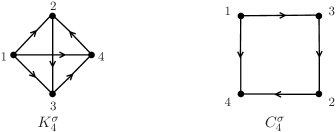
Figure 2.1: The orientations of $K_{4}$ and $C_{4}$ with the maximum skew energies

Example 2.9

Let $H=C_{4}$, $G_{0}=K_{4}$, $G_{1}=H\otimes G_{0}$, …, $G_{r}=H\otimes G_{r-1}$. It is obvious that $G_{r}$ is a $(3\cdot 2^{r})$-regular graph of order $4^{r+1}$. Then by Theorem 2.3, $G_{r}$ has the orientation with maximum skew energy $4^{r+1}\sqrt{3\cdot 2^{r}}$.

Example 2.10

Let $H=C_{4}$, $G_{0}=K_{4}$, $G_{1}=H\otimes G_{0}$, $G_{2}=G_{1}\otimes G_{0}$, …, $G_{r}=G_{r-1}\otimes G_{0}$. Note that $H$, $G_{1}$, $G_{2}$, …, $G_{r-1}$ are all regular bipartite graphs and $G_{r}$ is a $(2\cdot 3^{r})$-regular bipartite graph of order $4^{r+1}$. Then by Theorem 2.3, $G_{r}$ has the orientation with maximum skew energy $4^{r+1}\sqrt{2\cdot 3^{r}}$.

Example 2.11

Let $H=C_{4}$, $G_{0}=K_{4}$, $G_{1}=H\ast G_{0}$, …, $G_{r}=H\ast G_{r-1}$. Note that $G_{r}$ is a $(4\cdot 3^{r}-1)$-regular graph of order $4^{r+1}$. Then by Theorem 2.7, $G_{r}$ has the orientation with maximum skew energy $4^{r+1}\sqrt{4\cdot 3^{r}-1}$.

From Examples 2.9, 2.10 and 2.11, we can see that for some positive integers $k$, there exist oriented $k$-regular graphs with the maximum skew energy, which has order $n\leq k^{2}$. It is unknown that whether for any positive integer $k$, the oriented graph exists such that its order $n$ is less than $k^{2}$ and it has an orientation with the maximum skew energy.

2.3 The orientation of $H[G]$

In this subsection, we consider the lexicographic product $H[G]$ of a bipartite graph $H$ and a graph $G$. All definitions and notations are the same as above. We can see that the edge set $H[G]$ is the disjoint-union of the edge sets of $H\square G$ and $H\otimes K_{n}$, where $K_{n}$ is a complete graph of order $n$.

Let $H^{\tau}$ and $G^{\sigma}$ be oriented graphs of $H$ and $G$ with the skew-adjacency matrices $S_{1}$ and $S_{2}$, respectively. Let $K_{n}^{\varsigma}$ be an oriented graph of $K_{n}$ with the skew-adjacency matrix $S_{3}$. Then we can obtain two oriented graphs $(H^{\tau}\square G^{\sigma})^{o}$ and $(H^{\tau}\otimes K_{n}^{\varsigma})^{o}$. Thus it is natural to yield an orientation of $H[G]$, denoted by $H[G]^{o}$, such that the arc set of $H[G]^{o}$ is the disjoint-union of the arc sets of $(H^{\tau}\square G^{\sigma})^{o}$ and $(H^{\tau}\otimes K_{n}^{\varsigma})$. Let $\widetilde{S}$ be the skew-adjacency matrix of $H[G]^{o}$. We can see that $\widetilde{S}=\overline{S}+S^{\prime}_{1}\otimes S_{3}$, where $\overline{S}=I^{\prime}_{m_{1}+m_{2}}\otimes S_{2}+S_{1}\otimes I_{n}$ is the skew-adjacency matrix of $(H^{\tau}\square G^{\sigma})^{o}$. Then

$$\begin{split}\widetilde{S}^{T}\widetilde{S}&=-\widetilde{S}^{2}=-\left(\overline{S}+S^{\prime}_{1}\otimes S_{3}\right)^{2}\\ &=-\left[I_{m}\otimes S_{2}^{2}+S_{1}^{2}\otimes I_{n}+(S^{\prime}_{1})^{2}\otimes S_{3}^{2}+\overline{S}(S^{\prime}_{1}\otimes S_{3})+(S^{\prime}_{1}\otimes S_{3})\overline{S}\right]\\ &=-\left[I_{m}\otimes S_{2}^{2}+S_{1}^{2}\otimes I_{n}-S_{1}^{2}\otimes S_{3}^{2}+S_{1}\otimes(S_{2}S_{3})-S_{1}\otimes(S_{3}S_{2})\right]\end{split}$$

Suppose that $H^{\tau}$ is an oriented $k$-regular bipartite graph of order $m$ with maximum skew energy $m\sqrt{k}$. Then $S_{1}^{T}S_{1}=kI_{m}$. Let $G^{\sigma}$ be an oriented $l$-regular graph of order $n$ and maximum skew energy $n\sqrt{l}$. Then $S_{2}^{T}S_{2}=lI_{n}$. It is obvious that $H[G]^{o}$ is $(kn+l)$-regular. Moreover, let $K_{n}^{\varsigma}$ be an oriented graph of $K_{n}$ with maximum skew energy $n\sqrt{n-1}$. Then $S_{3}^{T}S_{3}=(n-1)I_{n}$, that is, $S_{3}$ is a skew-symmetric Hardamard matrix [8] of order $n$. If another condition that $S_{2}S_{3}=S_{3}S_{2}$ holds, then

$$\widetilde{S}^{T}\widetilde{S}=-\left[I_{m}\otimes S_{2}^{2}+S_{1}^{2}\otimes I_{n}-S_{1}^{2}\otimes S_{3}^{2}\right]=(kn+l)I_{mn}.$$

By Lemma 2.2, $H[G]^{o}$ has the maximum skew energy $mn\sqrt{kn+l}$.

The following example illustrates that the oriented graph satisfying the above conditions indeed exists.

Example 2.12

Let $H^{\tau}$ is an arbitrary oriented $k$-regular bipartite graph of order $m$ with the maximum skew energy $m\sqrt{k}$. Let $C_{4}^{\sigma}$ be the oriented graph of $C_{4}$ with maximum skew energy $4\sqrt{2}$ and the skew-adjacency matrix $S_{2}$, and $K_{4}^{\varsigma}$ be the oriented graph of $K_{4}$ with maximum skew energy $4\sqrt{3}$ and the skew-adjacency matrix $S_{3}$, see Figure 2.1. It can be verified that $S_{2}S_{3}=S_{3}S_{2}$. It follows that $(H[G])^{o}$ is an oriented $(4k+2)$-regular graph of order $4m$ with maximum skew energy $4m\sqrt{4k+2}$.

There are many options for $H$, such as $P_{2}$, $C_{4}$, $K_{4,4}$, the hypercube $Q_{d}$ and so on, which forms a new family of oriented graphs with the maximum skew energy.

References

- [1] C. Adiga, R. Balakrishnan, W. So, The shew energy of a digraph, Linear Algebra Appl. 432(2010), 1825–1835.
- [2] X. Chen, X. Li, H. Lian, -Regular oriented graphs with optimum skew energy, arXiv: 1304.0847.
- [3] X. Chen, X. Li, H. Lian, More on the skew-spectra of bipartite graphs and Cartesian products of graphs, arXiv: 1305.3414.
- [4] D. Cui, Y. Hou, On the skew spectra of Cartesian products of graphs, Electron. J. Combin. 20(2013), #P19.
- [5] S. Gong, G. Xu, -Regular digraphs with optimum skew energy, Linear Algebra Appl. 436(2012), 465–471.
- [6] I. Gutman, The energy of a graph, Ber. Math. Statist. Sekt. Forschungsz. Graz, 103(1978), 1–22.
- [7] X. Li, H. Lian, A survey on the skew energy of oriented graphs, arXiv: 1304.5707.
- [8] F.J. MacWilliams, N.J.A. Sloane, The Theory of Error-Correcting Codes, North-Holland, New York, 1977.
- [9] G. Tian, On the skew energy of orientations of hypercubes, Linear Algebra Appl. 435(2011), 2140–2149.