What exactly are the properties of scale-free and other networks?

Abstract

The concept of scale-free networks has been widely applied across natural and physical sciences. Many claims are made about the properties of these networks, even though the concept of scale-free is often vaguely defined. We present tools and procedures to analyse the statistical properties of networks defined by arbitrary degree distributions and other constraints. Doing so reveals the highly likely properties, and some unrecognised richness, of scale-free networks, and casts doubt on some previously claimed properties being due to a scale-free characteristic.

I Introduction

Scale-free networks are loosely defined to be networks where the number of connections per node has a power-law distribution Barabasi-Albert:scalefree . Such a definition is problematic because firstly the specification is vague, and secondly determining whether a histogram has a power-law distribution is notoriously difficult Clauset-etal:power-laws ; Goldstein-etal:power-laws ; Stumpf-Porter:power-laws ; Judd:dimension . Algorithms such as preferential attachment generate putative scale-free networks, but it is not clear that the networks are representative of typical scale-free networks Callaway-etal:graph-growth ; Catanzaro-etal:scale-free . Nor is it clear whether duplication models Pastor-Satorras-etal:node-duplication ; Chung-etal:node-duplication that model biological processes of network growth generate scale-free networks Bebek-etal:node-duplication , or suffer similar difficulties. Nonetheless, preferential attachment has become the de facto standard, and often treated as synonymous with scale-free.

Scale-free clearly refers to a statistical property of networks. Imagine a process that generates random graphs with specified properties, like being scale-free with power-law $\gamma$. Some characteristics of graphs can be prescribed precisely, like the number of nodes, or the minimum vertex degree. Other characteristics, like being scale-free with power-law $\gamma$, are truly statistical. These characteristics are specified probabilistically, such as by the probability of a number of nodes having certain degrees. For statistical properties like $\gamma$, it is not clear cut whether a graph has a specified $\gamma$ — unless one artificially adopts a particular way to measure $\gamma$. For statistical properties every graph should be assigned a probability of being generated by the process that generates random graphs with the specified property. Many graphs will have zero or negligibly small probability, but other graphs have a high probability, perhaps even for different but close values of $\gamma$.

This letter describes tools and procedures to explore random graphs with precisely defined properties. As an example we consider scale-free graphs with explicitly prescribed size $N$, power-law $\gamma>1$, and other characteristics, like minimum vertex degree $d$. With our tools we reveal previously unrecognised richness of scale-free graphs; figure 1 illustrates two examples that are unlike anything generated by preferential attachment. We discover that structural properties of scale-free graphs with $d=1$ fall into four categories according to three critical power-law values $\gamma_{0}\approx 2.47876$, $\gamma_{1}\approx 2.18482$, and $\gamma=2$, and an existence lower bound $\gamma>1$. We also show the critical effect minimum vertex degree $d$ has on the properties of scale-free graphs, and argue that some properties previously claimed to be due to scale-free characteristics are more likely due to effects of the minimum vertex degree $d$.

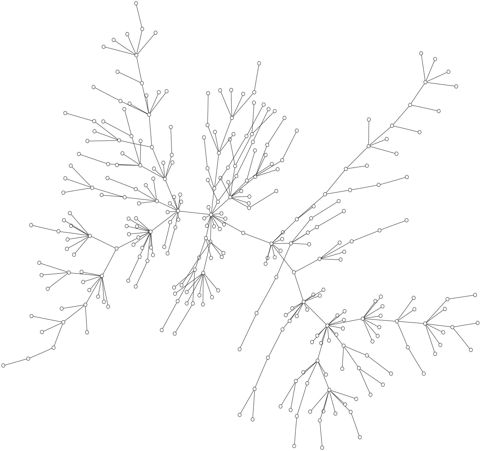
(a)  (b) 

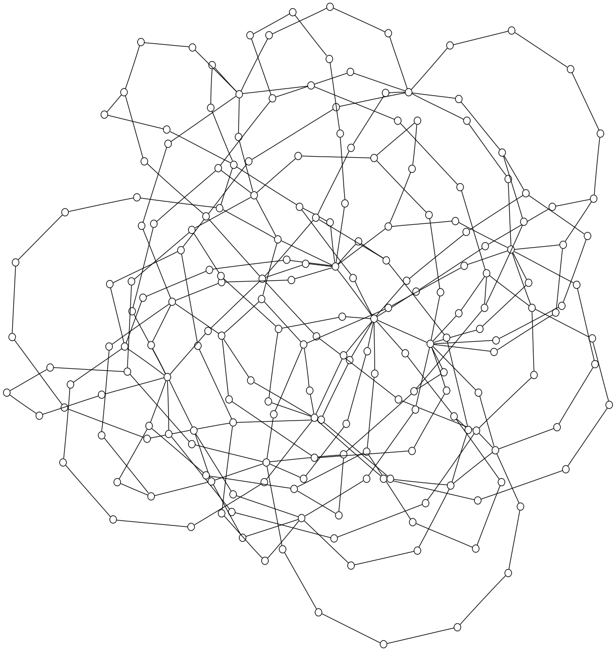
Figure 1: Two typical (high likelihood) random scale-free graphs of $300$ nodes with power-law $\gamma=2.4$, and minimum vertex degree (a) $d=1$, (b) $d=2$. Graph layout by neato North:neato .

II Characteristics defined by degree histograms

Our aim is to define processes to generate random graphs with specified properties; in particular graphs of a fixed size and prescribed distributions of vertex degrees.

Let ${\mathcal{G}}_{N}$ be the set of connected graphs with $N$ nodes and at most one edge between any pair of nodes. Since ${\mathcal{G}}_{N}$ is a finite set, then a process that randomly generates graphs with fixed characteristics is equivalent to assigning a probability mass $\Pr(G)$ to each graph $G\in{\mathcal{G}}_{N}$.

For $G\in{\mathcal{G}}_{N}$ let $n_{k}$ be the number of nodes of degree $k$, so that ${{\bf{n}}}(G)=(n_{1},\dots,n_{N-1})$ is the histogram of the degrees of the nodes of $G$. Let ${\mathcal{P}}({{\bf{n}}})\subseteq{\mathcal{G}}_{N}$ be the set of graphs with histogram ${{\bf{n}}}$. From a statistical point of view, if a characteristic depends only on ${{\bf{n}}}$, then any graph $G\in{\mathcal{P}}({{\bf{n}}})$ will serve as a representative of this characteristic. Hence, write the probability mass $\Pr(G)=\Pr(G|{{\bf{n}}})\Pr({{\bf{n}}})$, and stipulate that $\Pr(G|{{\bf{n}}})$ is the same for all graphs in ${\mathcal{P}}({{\bf{n}}})$. Then, graphs within ${\mathcal{P}}({{\bf{n}}})$ are equally likely, and are treated as equal representatives of the properties of ${\mathcal{P}}({{\bf{n}}})$. (The actual value of $\Pr(G|{{\bf{n}}})$ for $G\in{\mathcal{P}}({{\bf{n}}})$ is not important to the investigation, and is in practice rarely possible to compute. In the following $\Pr(G|{{\bf{n}}})$ is a normalisation that depends implicitly on other factors, like the sizes of the sets ${\mathcal{P}}({{\bf{n}}})$, which are extremely difficult to compute.)

Imagine then a process that randomly selects graphs from ${\mathcal{G}}_{N}$ such that there is a probability $p_{k}$ of a node having degree $k$ for each $k=1,\dots,N-1$. For graphs generated this way ${{\bf{n}}}(G)$ has a multinomial distribution,

$$\Pr({{\bf{n}}}(G))=N!\prod_{k=1}^{N-1}\frac{p_{k}^{n_{k}}}{n_{k}!}.$$ (1)

The methodology that follows can be applied to arbitrary degree distributions, and used to explore any statistical property that is determined by a degree distribution alone. A natural choice for the scale-free property is the zeta-distribution, where

$$p_{k}=\Pr(k|\gamma)=k^{-\gamma}/\zeta(\gamma),$$ (2)

where $k\geq 1$, $\gamma>1$ and $\zeta(\gamma)=\sum_{k=1}^{\infty}k^{-\gamma}$. The constant $\gamma$ defines the power-law. (Note: Eq. (2) implies $d=1$.)

III Generating random graphs

The question now is how to randomly generate scale-free graphs as we define. A Monte-Carlo Markov-chain (MCMC) approach can be used Fitzgerald:MCMC ; Gamerman:MCMC . Starting with an arbitrary initial graph $G\in{\mathcal{G}}_{N}$ one systematically proposes random simple modifications of the graph $G$ to produce a different graph $G^{\prime}\in{\mathcal{G}}_{N}$. The quantity

$$Q(G^{\prime}|G)=\frac{\Pr(G^{\prime})}{\Pr(G)}=\prod_{k=1}^{N-1}\frac{p_{k}^{n_{k}^{\prime}}}{n_{k}^{\prime}!}\frac{n_{k}!}{p_{k}^{n_{k}}},$$ (3)

measures the relative likelihood of the graphs. An MCMC approach accepts $G^{\prime}$ as a replacement for $G$ if $Q\geq 1$ and if $Q<1$, then $G^{\prime}$ is accepted with probability $Q$. Asymptotically, random graphs with the specified degree distribution (1) are obtained.

(a) $\gamma=1.5$, $X_{s}=175$	(b) $\gamma=2.0$, $X_{s}=46$
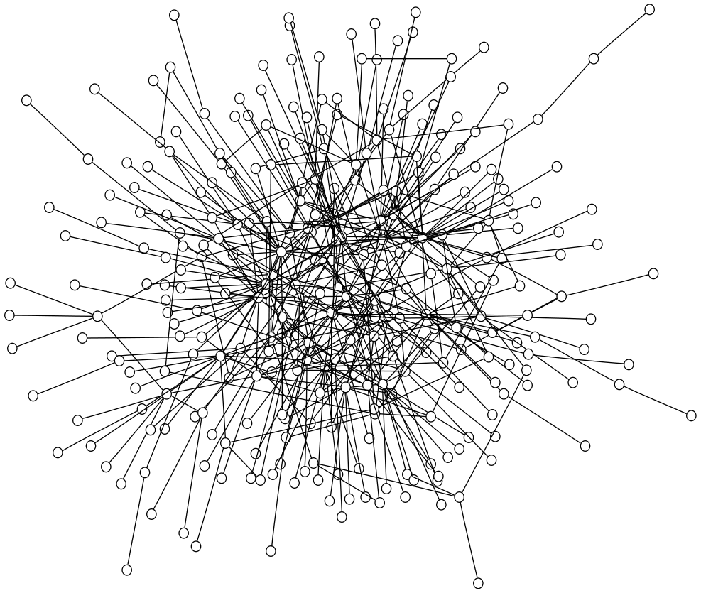
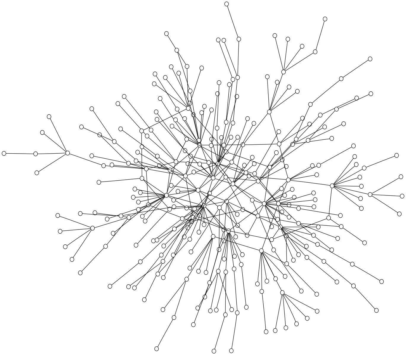
(c) $\gamma=2.5$, $X_{s}=6$	(d) $\gamma=3.0$, $X_{s}=0$

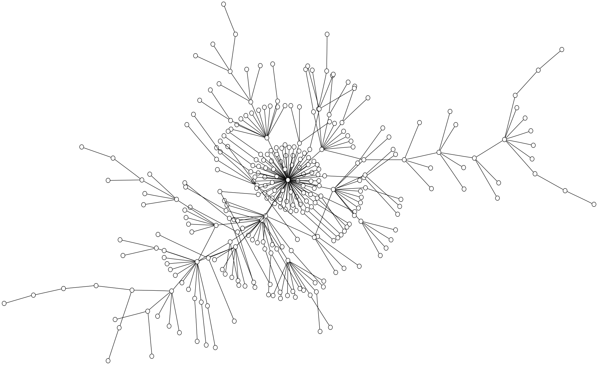
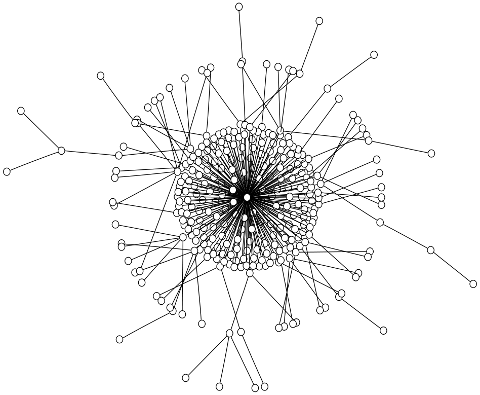
Figure 2: Random scale-free graphs with $N=300$, $d=1$, $\gamma$ as stated, using algorithm described in text. $X_{s}$ is the number of edges in excess of a spanning tree. Graph layout by neato North:neato .

The most basic modifications are adding and deleting a single edge. For example, if $G^{\prime}$ is obtained from $G$ by adding an edge between a node of degree $k$ and another node of degree $l$, where $|k-l|>1$, then $n_{k}$ and $n_{l}$ decrease by one, and $n_{k+1}$ and $n_{l+1}$ increase by one. Using (3) it can be easily derived that adding an edge $(s=1)$, or deleting an edge $(s=-1)$, between node of degree $k$ and another node of degree $l$, results in

$$Q=\begin{cases}\frac{n_{k}}{p_{k}}\frac{n_{l}}{p_{l}}\frac{p_{k+s}}{(n_{k+s}+1)}\frac{p_{l+s}}{(n_{l+s}+1)},&{}_{\text{$|k-l|>1$,}}\\[5.0pt] \frac{n_{k}}{p_{k}}\frac{p_{l+s}}{(n_{l+s}+1)},&{}_{\text{$k+s=l$,}}\\[5.0pt] \frac{n_{l}}{p_{l}}\frac{p_{k+s}}{(n_{k+s}+1)},&{}_{\text{$k=l+s$,}}\\[5.0pt] \frac{n_{k}(n_{k}-1)}{p_{k}^{2}}\frac{p_{k+s}^{2}}{(n_{k+s}+2)(n_{k+s}+1)},&{}_{\text{$k=l$, $n_{k}\geq 2$.}}\end{cases}$$ (4)

For scale-free graphs substitute (2) into (4), and note that the zeta functions cancel out entirely.

Adding and deleting edges is transitive in ${\mathcal{G}}_{N}$, but another useful modification that accelerates convergence is to disconnect one or more edges from a node, and reconnect these edges to other nodes. Consider the simplest case where a giver node has degree $k$, that $m<k$ edges are disconnected and these are all reconnected to a receiver node of degree $l$; we will call such modifications gifting. The degrees of the giver and receiver nodes decrease and increase respectively by $m$; it follows that since necessarily $n_{k},n_{l}\geq 1$, then

$$Q=\begin{cases}\frac{n_{k}}{p_{k}}\frac{p_{k-m}}{(n_{k-m}+1)}\frac{n_{l}}{p_{l}}\frac{p_{l+m}}{(n_{l+m}+1)},&{}_{\text{$k-l\neq 0,m,2m$,}}\\[4.0pt] \frac{n_{k}(n_{k}-1)\ {}p_{k-m}\ {}p_{k+m}}{p_{k}^{2}\ {}(n_{k-m}+1)(n_{k+m}+1)},&{{}_{\text{$k=l$, $n_{k}\geq 2$,}}}\\[4.0pt] 1,&{}_{\text{$k=l+m$,}}\\ \frac{n_{k}}{p_{k}}\frac{n_{l}}{p_{l}}\frac{p_{k-m}^{2}}{(n_{k-m}+1)(n_{k-m}+2)},&{{}_{\text{$k-m=l+m$.}}}\end{cases}$$ (5)

Substitution of (2) gives $Q$ for scale-free graphs.

Care is required making any modification to a graph because it can result in graphs that are not in ${\mathcal{G}}_{N}$. Given the assumed properties of ${\mathcal{G}}_{N}$ an edge can only be added if the nodes are not already connected, and deletion of an existing edge is only allowed if the resulting graph is connected. Gifting can also result in disconnected graphs. Ensuring the graph is connected is a somewhat involved process, and somewhat tangential to our interests, so to avoid disrupting our narrative we will deal with this detail later when describing the algorithm used in our calculations.

IV Properties of scale-free graphs

We have introduced some basic methods of modifying graphs in ${\mathcal{G}}_{N}$ to obtain different graphs in ${\mathcal{G}}_{N}$. These can be used in an MCMC approach, but an MCMC approach can be slow to converge, especially if the arbitrary initial graph is far from being scale-free. An alternative approach is to seek highly likely graphs by maximising $\Pr(G)$. This can be achieved by considering various modifications of $G$ and selecting the modification that has the largest $Q$. Our algorithm to implement gradient ascent of $Q$, which is used in our calculations, is described and discussed later.

So then, we come to answer the question in the title. Figure 2 shows highly likely scale-free graphs obtained using the gradient ascent algorithm stated later; these graphs are typical representatives. We find there is a significant subset of scale-free graphs that are trees, especially for larger $\gamma$ values. For intermediate $\gamma$ scale-free graphs are similar to scale-free trees with some extra edges linking nodes, which break the tree structure by creating loops. For smaller $\gamma$ values the proportion of edges creating loops increases.

This tree-like nature deserves closer attention, because it has been noted elsewhere Kim-etal:scalefree-trees . If $G\in{\mathcal{G}}_{N}$, then a spanning tree $S(G)$ of $G$ has exactly $N-1$ edges, so the number of edges ${\mathcal{E}}(G)$ of $G$ in excess of ${\mathcal{E}}(S(G))=N-1$ is an indication of the amount of cross-linking. Excesses are stated for the graphs in figure 2. On the other hand, the expected excess $X_{s}(G)={\mathcal{E}}(G)-{\mathcal{E}}(S(G))$ for scale-free graphs in ${\mathcal{G}}_{N}$ with $\gamma>2$, $d=1$, is

$$E[X_{S}(G)]=N\times\left(\frac{1}{2}\frac{\zeta(\gamma-1)}{\zeta(\gamma)}-1\right)+1.$$ (6)

The quantity in brackets is decreasing, diverging to positive infinity as $\gamma$ approaches 2 from above, negative for $\gamma>\gamma_{0}\approx 2.47876$, and equal to one at $\gamma=\gamma_{1}\approx 2.18482$.

The expected excess (6) implies that for $\gamma>\gamma_{0}$ scale-free graphs are always expected to be trees. In fact, there should be a deficit of edges, which forces scale-free graphs toward the extreme of one node of very large degree and many nodes of degree one, like figure 2(d). For $\gamma_{1}<\gamma<\gamma_{0}$ scale-free graphs are expected to have less cross-links than links in a spanning tree, and so are tree-like. For $\gamma<\gamma_{1}$ there are expected to be more cross links than spanning tree links, so the graphs are not expected to be tree-like, and are frequently observed in real world networks Kim-etal:scalefree-trees . For $\gamma>2$ the excess is expected to be a bounded multiple of the number of nodes $N$. When $\gamma<2$ the expected number of links grows without bound as $N$ increases until nearly fully connected graphs are produced. These far from tree-like graphs have been termed dense DelGenio-etal:scale-free , but, contrary to the claim of the cited work, there are many such dense graphs for any $N$ and $1<\gamma<2$; our supplied algorithm finds them easily, because it searches within the set of graphs ${\mathcal{G}}_{N}$, rather than by histogram.

${\mathcal{E}}_{0}$	${\mathcal{E}}_{*}$	$\log{P}$	Add	Del.	Gift	Total	Lower	Upper
$\gamma=1.5$
300	482	-87.41	183	1	61	245	43	558
400	475	-87.69	100	25	81	206	97	742
500	504	-86.97	36	32	82	150	129	970
600	574	-86.82	22	48	101	171	144	1248
700	626	-87.75	20	94	117	231	164	1526
$\gamma=2.0$
300	303	-33.75	6	3	31	40	43	306
400	336	-35.35	7	71	59	137	119	648
500	385	-39.59	14	129	93	236	164	1018
600	418	-43.03	12	194	135	341	177	1258
700	458	-47.41	27	269	194	490	205	1622
$\gamma=2.5$
300	299	-31.88	2	3	67	72	64	424
400	313	-32.41	5	92	103	200	159	876
500	341	-38.36	8	167	137	312	176	1164
600	359	-44.54	12	253	155	420	208	1402
700	427	-58.79	29	302	179	510	226	1790

Table 1: Typical behaviour of gradient ascent of $Q$ for a graph of $N=300$ nodes. Columns are: ${\mathcal{E}}_{0}$ and ${\mathcal{E}}_{*}$, initial and final number of edges; $\log{P}$, final log-likelihood; number of additions, deletions, and gifting moves; total moves and predicted lower and upper bounds on number of moves. Recall that the excess links over a tree is $X_{S}={\mathcal{E}}_{*}-N+1$.

We conclude that random scale-free graphs with $d=1$ and $\gamma_{1}<\gamma<\gamma_{0}$ are best characterized as having an under-lying, more-or-less scale-free, tree, and are expected to be scale-free trees for $\gamma>\gamma_{0}$, and nodes with very large degree for larger $\gamma$. These characteristic structures are well illustrated in figure 2. Furthermore, the characteristics are confirmed by observing the relative frequency of the different modifications during the likelihood ascent. Table 1 compiles a summary of the typical behaviour of likelihood ascent. For $\gamma=1.5$, the non-tree like case with many cross-links, the likelihood ascent is mainly adding and gifting edges. For $\gamma=2.5$, the tree-like case with few cross-links, the likelihood ascent is mainly deleting and gifting edges.

V Generating large graphs

We have introduced means to obtain scale-free graphs by modification of an initial graph. Given our conclusion that scale-free graphs for $\gamma>\gamma_{1}$ are essentially tree-like, this suggests an alternative constructive approach for building random scale-free graphs by adding individual nodes with one link.

If a graph $G\in{\mathcal{G}}_{N}$ is modified by adding a node with one link to an existing node of degree $k$, then a new graph $G^{\prime}\in{\mathcal{G}}_{N+1}$ is created with

$$Q=\begin{cases}{\scriptstyle(N+1)}\frac{p_{1}}{n_{1}+1}\frac{n_{k}}{p_{k}}\frac{p_{k+1}}{n_{k+1}+1},&k>1,\\[5.0pt] {\scriptstyle(N+1)}\frac{p_{2}}{n_{2}+1},&k=1,\end{cases}$$ (7)

which follows from Eq. (1) similar to (3). Hence, Eq. (7) provides an optimal preferential attachment rule, however, attachment rules alone need not result in highly likely graphs Callaway-etal:graph-growth . Locally optimum graphs can be obtained if after one or more attachments the link modifications previously described are used.

Figure 3 shows the growth of excess links $X_{s}(G)$, for $G\in{\mathcal{G}}_{N}$ constructed in this way with Eq. (7) used as the attachment rule. The staircase shape results from occasional avalanches of link modifications after a period of mainly node-link additions with few modifications. There appears to be a self-organised criticality.

For $1<\gamma<2$ the excess should grow without bound until the graph is almost fully connected, but figure 3 clearly shows the number of nodes needs to be many orders of magnitude before this effect is apparent; only $\gamma=1.5$ has more cross-links than spanning-tree links for $N>600$ nodes. For $2<\gamma<\gamma_{0}$ the growth of $X_{s}(G)$ should become asymptotically linear in $N$, that is, a constant proportion of cross-links. Once again, graphs many orders of magnitude larger are required before this effect is apparent.

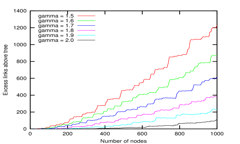
Figure 3: Excess links over those of a spanning tree $X_{S}(G)$ of random scale-free graphs with $N$ nodes, computed by optimal additions and local likelihood ascent for various $\gamma$.

VI Algorithm

We now state and discuss the algorithm used in the computations. This algorithm sequentially modifies the links of a given graph to obtain another graph with the same number of nodes but higher likelihood of being scale-free. Links are modified by the three operations of adding, deleting, and gifting. The algorithm requires only the number of nodes $N$ and the target degree distribution, which in the case of (2) is defined by the single power-law parameter $\gamma$.

Steps 3 and 4 treat the current graph $G$ as a representative of an equivalence class of graphs having node-degree histogram ${{\bf{n}}}(G)$; these two steps determine which equivalence classes are accessible from $G$ using the allowed modifications, and which achieve the largest increase in $Q$. Steps 5 and 6 determine if there is a specific valid modification of $G$ that can make the potentially best transition to another equivalence class.

The following notation is used: $G\in{\mathcal{G}}_{N}$ is the current graph with nodes numbered 1 to $N$; $A$ is the adjacency matrix of $G$, $A_{ij}=1$ if node $i$ is linked to $j$, zero otherwise; $a_{i}$ is column $i$ of $A$; $I_{k}$ is the set of nodes with degree $k$, by definition $n_{k}=|I_{k}|$ and $i\in{}I_{k}$ iff $\|a_{i}\|_{1}=k$; ${\mathcal{N}}_{i}=\{j\colon{}A_{ij}=1\}$, the nodes linked to node $i$; $C(i,j,{\mathcal{L}})=1$ if there exists a path between node $i$ and $j$ after the links in ${\mathcal{L}}$ have been deleted, and zero otherwise.

1. Choose an arbitrary initial graph $G\in{\mathcal{G}}_{N}$.

2. Compute the node-degree histogram ${{\bf{n}}}(G)$ and log-likelihood $\log\Pr({{\bf{n}}}(G))$.

3. Choose a degree $k$ such that $n_{k}>0$; chosen uniformly amongst non-zero $n_{k}$.

4. Compute $\log{}Q_{klm}$ for all potentially valid $k$, $l$, $m$, that is all possible changes involving a node of degree $k$ and another of degree $l$, where $m$ identifies the type of change: ($m=\mathcal{A}$) addition of a link, Eq. (4); ($m=\mathcal{D}$) deletion of a link, Eq. (4); ($m\in{\mathbb{Z}}^{+}$) gift $m$ links from a node of degree $k$ to a node of degree $l$, Eq. (5).

5. Check the list of $\log{}Q_{klm}>0$ in descending order of magnitude for the first valid change, if none, return to step 3. Validity is tested as follows. Find candidate nodes $i\in{}I_{k}$, $j\in{}I_{l}$, for the change as follows:

   1. $A_{ij}=0$;

   2. $A_{ij}=1$ and $C(i,j,\{(i,j)\})=1$;

   3. $a_{i}^{T}a_{j}-A_{ij}\leq{}n_{k}-m$.

   If there is more than one pair of $(i,j)$ then choose uniformly randomly between then. This is achieved by choosing uniformly random permutations Knuth:fundamental-algorithms of the elements of $I_{k}$ and $I_{l}$, then running over $i$ in permutation order with an embedded loop over $j$ in permutation order until the first valid pair is found.

6. Make the valid change to $G$ and return to step 2. For addition ($c=1$) and deletion ($c=0$), set $A_{ij}=A_{ji}=c$. Step 5($m$) ensures that $m$ nodes linked to node $i$ can be moved to node $j$, however, some choices of the $m$ nodes can result in disconnected graphs. Proceed as follows:

   1. If $A_{ij}=0$ and $a_{i}^{T}a_{j}=0$, then choose uniformly randomly from $h\in{\mathcal{N}}_{i}$ where $C(j,h,\{(i,g)\colon{}g\in{\mathcal{N}}_{i}\})=1$. Otherwise, set $h=j$.

   2. Choose $m$ nodes uniformly randomly from $\{g\in{\mathcal{N}}_{i}\colon{}g\not\in{\mathcal{N}}_{j},g\not={}h\}$. Relink these nodes by setting $A_{ig}=A_{gi}=0$ and $A_{jg}=A_{gj}=1$.

The algorithm employs the test $C(i,j,{\mathcal{L}})$ for a graph $G$ as to whether node $i$ is connected to node $j$ when the links in ${\mathcal{L}}$ are removed. The purpose of this test is to ensure that a graph remains connected after some change to the graph. A graph $G$ is connected if the matrix $C_{p}=I+A+A^{2}+\cdots+A^{p}$ has no zero elements for $p=N-1$. A pair of nodes $i$ and $j$ is connected by a path if there exists $p<N$ such that $C_{pij}\not=0$. If $a_{i}$ and $a_{j}$ are columns $i$ and $j$ of $A$ respectively, $w_{p+1}=Aw_{p}+w_{p}$, and $w_{1}=a_{j}$, then $C_{pij}=a_{i}^{T}w_{p}$, which is a relatively efficient computation for each $p$. Hence, $C(i,j,{\mathcal{L}})$ requires computing $C_{pij}$ where $A$ is modified so that $A_{uv}=A_{vu}=0$ for each $(u,v)\in{\mathcal{L}}$.

The algorithm should terminate at a local optimum of $\log\Pr({{\bf{n}}})$ when either $\log{}Q_{klm}$ is non-positive for all $klm$, or there are no valid changes with $\log{}Q_{klm}>0$ for any $klm$. However, step 3 makes a random choice of $k$, so as stated the algorithm will not terminate and requires an additional stopping criterion. For example, if more than a prescribed number of trials of $k$ result in no valid changes, then test each $k$ with $n_{k}>0$ sequentially, if none results in valid changes then a local optimum of $\log\Pr({{\bf{n}}})$ has been reached.

VII Algorithm performance

We provide here some comments on the performance of the algorithm. The histogram $\widehat{{\bf{n}}}$ that maximizes $\Pr({{\bf{n}}})$ for the multinomial distribution (1), has $\widehat{n}_{k}\approx{}Np_{k}$. Substituting into (3) and using Stirling’s approximation of a factorial, obtains

$$Q(\widehat{G}|G)\approx\prod_{k=1}^{N-1}\left(\frac{n_{k}}{\widehat{n}_{k}}\right)^{n_{k}+\frac{1}{2}}.$$ (8)

This approximation assumes $n_{k}\neq\widehat{n}_{k}$ only if $n_{k}\gg 1$. The expressions (4), (5) and (7) for $Q$, were the result of small changes to graphs, but (8) it can be seen that modest deviations from $n_{k}\approx\widehat{n}_{k}$ can result in significant change in probability mass. Hence, most graphs in ${\mathcal{G}}_{N}$ do not display the scale-free property. On the other hand, there are a lot of scale-free graphs Bekassy-etal:enumeration ; vanderHofstad:2006 ; Catanzaro-etal:scale-free , the number of which can be estimated as follows. Consider constructing a graph by choosing $n_{k}\approx\widehat{n}_{k}$ and assigning degrees to the nodes, then adding links randomly first to obtain a tree from the nodes, then to achieve the chosen degrees of the nodes. An upper bound on the number of graphs can be computed from combinatorial analysis of this method, see references; it is an upper bound because it is difficult to ensure the constructed graph is in ${\mathcal{G}}_{N}$.

Of importance to gradient ascent of $Q$ is an estimate of the number of moves required to reach a high-likelihood scale-free graph $\widehat{G}$ with ${{\bf{n}}}(\widehat{G})=\widehat{{\bf{n}}}$ from an initial graph $G$. A lower-bound on the number of moves required is around $\frac{1}{2}\sum_{k=1}^{N-1}|n_{k}-\widehat{n}_{k}|$; here each move corrects the degrees of a pair nodes. A worst case upper-bound is around $\frac{1}{2}\sum_{k=1}^{N-1}k|n_{k}-\widehat{n}_{k}|$, where a move is required to relocate each edge end. The lower-bound should be tight, the upper-bound is expected to be typically an significant over-estimate. These upper and lower bounds are include in Table 1 for comparison the actual number of steps our algorithm took; it can be seen that in all cases the algorithm is closer to the lower bound than the upper bound.

Table 1 also shows that when the initial graph has minimal edges, then near optimal graphs are obtained, but when the initial graph has much too many edges, then the algorithm often gets caught in good, but sub-optimal, graphs. This suggests building a graph up is more effective than reducing a graph down. In the latter case some initial deletions can leave the graph in a configuration that cannot be easily corrected; note the large number of additions and deletions in these case in table 1, which results from frequent readjustment from earlier deletions. The optimal starting condition appears to have as many edges as the optimal graph, which minimises additions and deletions, which can be predicted in advance. Another disadvantage of initial graphs with too many edges, not revealed by table 1, is that they require many more evaluations of potential $Q$ values, meaning individual moves take longer.

VIII Conclusion

We have presented a methodology and specific algorithm for constructing finite random scale-free graphs with minimum node degree $d=1$. Calculation and subsequent analysis reveals four scale ranges with statistically different properties. Based on our evidence we conclude that scale-free graphs are not particularly robust to deletions for $\gamma>\gamma_{1}$, being based on an under-lying tree; any robustness derives from the cross-linking, which is more prevalent for smaller $\gamma$ values, but expected to be entirely absent for $\gamma>\gamma_{0}$. This brings into question some qualities, like robustness and clustering, that have been claimed to be due to the scale-free property of graphs. Our evidence suggests that additional, often implicit, assumptions and constraints, such as, a minimum degree of nodes $d>1$ are responsible.

This strong effect of $d$ highlights a potential mis-conception. Usually when power-laws arise (phase transitions, Hirsch exponent, fractal dimension, extreme events, self-organized criticality) the asymptotics of the distribution dominates the interesting physics. Here, it seems, the properties of the most numerous nodes are important too, that is, the shape of the left side of the degree histogram, rather than the tail on the right. These effects can be explored using the methods we have presented. It should be possible to make further characterizations of random graphs under different probability constraints on the degrees of nodes. The methodology presented here can be adapted to cases of $d>1$; figure 1(b) was obtained by applying the described algorithm with a shifted zeta-distribution, where $p_{1}=\cdots=p_{d-1}=0$ and

$$p_{k}=(k-d+1)^{-\gamma}/\zeta(\gamma),\quad{}k\geq{}d.$$ (9)

The three basic graph modifications of addition, deletion and gifting, were sufficient for $d=1,2$, but different modifications will be required for efficient algorithms for $d>2$.

References

- (1) A.L. Barabasi and R. Albert. Emergence of scaling in random networks. Science, 286:509–512, 1999.
- (2) A. Clauset, C.R. Shalizi, and M.E.J. Newman. Power-law distributions in empirical data. SIAM Review, 51:661–703, 2009.
- (3) M.L. Goldstein, S.A. Morris, and G.G. Yen. Problems with fitting the power law distribution. European Physics Journal B, 41:255–258, 2004.
- (4) M.P.H. Stumpf and M.A. Porter. Critical truths about power laws. Science, 335:665–666, 2012.
- (5) K. Judd. An improved estimator of dimension and some comments on providing confidence intervals. Physica D, 56:216–228, 1992.
- (6) D.S. Callaway, J.E. Hopcroft, J.M. Klienberg, M.E.J Newman, and S.H. Strogatz. Are randomly grown graphs really random? Physical Review E, 64:041902, 2001.
- (7) M. Catanzaro, M. Boguñá, and R. Pastor-Satorras. Generation of uncorrelated random scale-free networks. Physical Review E, 71:027103, 2005.
- (8) R. Pastor-Satorras, E. Smith, and R.V. Solé. Evolving protien interaction networks through gene duplication. Journal of Theoretical Biology, 222:199–210, 2003.
- (9) F. Chung, L. Lu, T.G. Dewey, and D.J. Galas. Duplication models for biological networks. Journal of Computational Biology, 10(5):677–687, 2003.
- (10) G. Bebek, P. Berenbrink, C. Cooper, T. Friedetzky, J. Nadeau, and S.C. Sahinalp. The degree distribution of the generalized duplication model. Theoretical Computer Science, 369:234–249, 2006.
- (11) S.C. North. Drawing graphs with neato. Technical report, www.graphviz.org, 2004.
- (12) R. Fitzgerald. Numerical bayesian methods applied to signal processing. Springer, 1997.
- (13) D. Gamerman. Markov Chain Monte Carlo: Stochastic Simulation for Bayesian Inference. Chapman & Hall, 1997.
- (14) D.H. Kim, J.D. Noh, and H. Jeong. Scale-free trees: the skeletons of complex networks. Physical Review E, 70:046126, 2004.
- (15) C.I. Del Genio, T. Gross, and K.E. Bassler. All scale-free networks are sparse. Physical Review Letters, 107:178701, 2011.
- (16) D. E. Knuth. Fundamental Algorithms, volume 1. Addison-Wesley, Reading, Massachussetts, 2nd edition, 1973.
- (17) A. Bekassy, P. Bekessy, and J. Komlos. Asymptotic enumeration of regular matrices. Stud. Sci. Math. Hung., 7:343–, 1972.
- (18) Remco van der Hofstad and Joel Spencer. Counting connected graphs asymptotically. Eur. J. Comb., 27(8):1294–1320, November 2006.