FTPI-MINN-13/17, UMN-TH-3205/13

May 29/2013

Calculating Extra (Quasi)Moduli on the
Abrikosov-Nielsen-Olesen string with
Spin-Orbit Interaction

Sergei Monin,^a M. Shifman,^b A. Yung^b,c

^aDepartment of Physics, University of Minnesota, Minneapolis, MN 55455, USA

^bWilliam I. Fine Theoretical Physics Institute, University of Minnesota, Minneapolis, MN 55455, USA

^cPetersburg Nuclear Physics Institute, Gatchina, St. Petersburg 188300, Russia

Abstract

Using a representative set of parameters we numerically calculate the low-energy Lagrangian on the world sheet of the Abrikosov-Nielsen-Olesen string in a model in which it acquires rotational (quasi)moduli. The bulk model is deformed by a spin-orbit interaction generating a number of “entangled” terms on the string world sheet.

1 Introduction

In the previous publications simple models with “spin-orbit” interactions supporting the Abrikosov-Nielsen-Olesen (ANO) [2] or similar strings (vortices) were considered [3, 4, 5] with “extra” non-Abelian moduli (or quasimoduli) on the string world sheet. Such extra moduli fields can appear in the bulk models that have order parameters carrying spatial indices, such as those relevant for superfluidity in ³He (see e.g. [6]). This particular example was studied in [4], which, in fact inspired a more detailed numerical analysis presented below. The studies in [3, 4, 5] were carried out at a qualitative level. Here we perform calculations needed for the proof of stability of the relevant solutions and derivation of all constants appearing in the low-energy theory on the string world sheet.

First, we will consider the simplest model [3] assuming weak coupling in the bulk (to justify the quasiclassical approximation), determine the profile functions to find the string solution, and derive the world sheet model. The general theory of the string moduli in the absence of the spin-orbit terms is discussed in [7, 8].

Then we introduce a spin-orbit interaction in the bulk. The impact of this interaction on the string (vortex) world sheet amounts to lifting all or some rotational zero modes (i.e. those not associated with the spontaneous breaking of the translational symmetry by the string). However, under certain condition on a parameter determining the spin-orbit interaction in the bulk, the mass gap generated on the world sheet remains small, and the extra zero modes survive as quasizero modes (some may remain at zero at the classical level). In addition to the above mode-lifting, the spin-orbit interaction generates a number of interesting entangled terms on the string world sheet which couple rotational and translational modes (despite the fact that the translational modes remain exactly gapless).

2 Formulation of the problem

We start from the model suggested in [3]. Its overall features are similar to those of the superconducting cosmic strings [9]. The model is described by an effective Lagrangian

$${\cal L}={\cal L}_{0}+{\cal L}_{\chi}$$ (1)

where

$${\cal L}_{0} = -\frac{1}{4e^{2}}F_{\mu\nu}^{2}+\left|{\mathcal{D}}^{\mu}\phi\right|^{2}-V(\phi)\,,$$

$${\mathcal{D}}_{\mu}\phi = (\partial_{\mu}-iA_{\mu})\phi\,,$$

$$V = \lambda\left(|\phi|^{2}-v^{2}\right)^{2}\,,$$ (2)

and

$${\cal L}_{\chi} = \partial_{\mu}\chi^{i}\,\partial^{\mu}\chi^{i}-U(\chi,\phi)\,,$$ (3)

$$U = \gamma\left[\left(-\mu^{2}+|\phi|^{2}\right)\chi^{i}\chi^{i}+\beta\left(\chi^{i}\chi^{i}\right)^{2}\right],$$ (4)

with self-evident definitions of the fields involved, the covariant derivative, and the kinetic and potential terms. The parameters $e$, $\lambda$, $\beta$, $\mu$, and $v$ can be chosen at will, with some mild constraints (e.g. $v>\mu$) discussed in [4]. In particular, the stability of the $\phi\neq 0$ vacuum we are interested in implies that $\beta$ cannot be too small,

$$\beta\geq\frac{m_{\chi}^{2}}{m_{\phi}^{2}}\,\frac{1}{c(c-1)}\,,$$ (5)

where

$$c\equiv\frac{v^{2}}{\mu^{2}}\,,$$ (6)

cf. Eq. (9). The relations between the parameters in (2), (4) and $a,b,c$ appearing below, on the one hand, and the physical parameters (the particle masses and the coefficients in front of the quartic terms $\phi^{4}$, $\chi^{4}$ and $\phi^{2}\chi^{2}$, respectively), on the other hand, are shown in Table 1 and (7), (9).

$\beta$	$\displaystyle\frac{\tilde{\lambda}}{\gamma}$
$a$	$\displaystyle\frac{m_{A}^{2}}{m_{\phi}^{2}}$
$b$	$\displaystyle\frac{m_{\chi}^{2}}{m_{\phi}^{2}}$
$\displaystyle\frac{v^{2}}{\mu^{2}}\equiv c$	$\displaystyle\left(1-\frac{4\lambda}{\gamma}\frac{m_{\chi}^{2}}{m_{\phi}^{2}}\right)^{-1}$

Table 1: Parameters in (2), (4) in terms of the particle masses and the coefficients in front of the quartic terms $\phi^{4}$, $\chi^{4}$, and $\phi^{2}\chi^{2}$ ($\lambda$, $\tilde{\lambda}$, and $\gamma$, respectively).

We will assume the parameters to be chosen in such a way that the bulk model is weakly coupled and, hence, the quasiclassical approximation is applicable.

Now let us discuss some parameters and the corresponding notation. In the vacuum the complex field $\phi$ develops a vacuum expectation value $|\phi_{\rm vac}|=v$ while its phase is eaten up by the Higgs mechanism. The masses of the (Higgsed) photon and the Higgs excitation are

$$m^{2}_{A}=2e^{2}v^{2}\,,\quad m^{2}_{\phi}=4\lambda v^{2}\,.$$ (7)

We will denote the ratio of the masses

$$a=m^{2}_{A}/m^{2}_{\phi}\equiv\frac{e^{2}}{2\lambda}\,\,.$$ (8)

Moreover, in the vacuum the field $\chi^{i}$ does not condense. Its mass is

$$m^{2}_{\chi}=\gamma\left(v^{2}-\mu^{2}\right).$$ (9)

For what follows we will introduce two extra dimensionless parameters:

$$b=m^{2}_{\chi}/m^{2}_{\phi}\equiv\frac{\gamma}{4\lambda}\,\frac{c-1}{c}\,,\quad c=v^{2}/\mu^{2}\,.$$ (10)

The first measures the ratio of the $\chi$ to $\phi$ masses in the bulk and, as explained in [3], has to be $b\lower 3.01385pt\hbox{$\;\stackrel{{\scriptstyle\textstyle>}}{{\sim}}\;$}1$. The second parameter is also constrained, $c>1$. We will treat both of them as parameters of the order of unity. As for the spatial orientation, the string will be assumed to lie along the $z$ axis. We introduce a dimensionless radius in the perpendicular $\{x,y\}$ plane,

$$\rho=m_{\phi}\,\sqrt{x^{2}+y^{2}}\,.$$ (11)

The basis of our construction is the standard ANO string (see e.g. [10]). The $\phi$ field winds ensuring topological stability, which entails in turn its vanishing at the origin. This implies the following ansätze:

$$A_{0}=0\,,\quad A_{i}=-\varepsilon_{ij}\frac{x_{j}}{r^{2}}\left(\rule{0.0pt}{11.38109pt}1-f(r)\right)\,,\quad\phi=v\varphi(\rho)e^{i\alpha}\,,$$ (12)

where $\alpha$ is the polar angle in the perpendicular plane, and we assume for simplicity the minimal (unit) winding. The boundary conditions supplementing (12) are

$$f(\infty)=0\,,\qquad f(0)=1\,;\qquad\,\varphi(\infty)=1\,,\quad\varphi(0)=0\,.$$ (13)

In the core of such a tube the $\phi$ field tends to zero, see (13). The vanishing of the $\phi$ field results in the $\chi^{i}$ field destabilization in the core of the string (as follows from Eq. (4)). Hence, inside the core, the $\chi^{i}$ field no longer vanishes,

$$(\chi^{i}\chi^{i})_{\rm core}\approx\frac{\mu^{2}}{2\beta}\,,$$ (14)

as will be illustrated by the graphs given below. Choosing the value of $\lambda$ judiciously, we can make $\mu^{2}/\beta\gg m_{\chi}^{2}$, implying that the O(3) symmetry is broken in the core. The appropriate ansatz is

$$\chi^{i}=\frac{\mu}{\sqrt{2\beta}}\,\chi(\rho)\left(\begin{array}[]{c}0\\ 0\\ 1\end{array}\right)\,,$$ (15)

with the boundary conditions

$$\chi(\infty)=0\,,\quad\chi(0)\approx 1\,.$$ (16)

Thus, we have three profile functions, $f$, $\varphi$, and $\chi$, depending on $\rho$. Minimizing the energy functional we derive the system of equations for the profile functions

$$\left(\frac{f^{\prime}}{\rho}\right)^{\prime} = a\frac{\varphi^{2}\,f}{\rho}\,,$$

$$\left(\rule{0.0pt}{11.38109pt}\phi^{\prime}\rho\right)^{\prime} = \frac{f^{2}\,\varphi}{\rho}+\frac{\rho\varphi\left(\varphi^{2}-1\right)}{2}+\frac{\rho\,\varphi\,\chi^{2}}{2\beta}\frac{b}{c-1}\,,$$

$$\left(\rule{0.0pt}{11.38109pt}\chi^{\prime}\rho\right)^{\prime} = \frac{b}{c-1}\rho\chi\left(c\varphi^{2}+\chi^{2}-1\right)\,,$$ (17)

where the primes denote differentiation with respect to $\rho$. In the numerical solution to be presented below we will assume for simplicity that

$$a=1\,,\,\,\,\mbox{ i.e.}\,\,\,m_{\phi}=m_{A}\,.$$ (18)

In the absence of the $\chi$ filed this would imply the Bogomol’nyi-Prasad-Sommerfield (BPS) limit [11] with the tension 

$$T_{0}=2\pi v^{2}\,.$$ (19)

Below we will see how the presence of the $\chi$ filed changes the tension, using $T_{0}$ as a reference point.

It is obvious that the solution $\chi=0$ and $\varphi=\varphi_{0}\equiv\varphi_{\rm ANO}$ satisfies the set of equations (17). First we will show that this solution is unstable, i.e. corresponds to the maximum rather than minimum of the energy functional.

3 Instability of the $\chi=0$ solution

To prove instability we must demonstrate that for $\varphi=\varphi_{0}\equiv\varphi_{\rm ANO}$ there is a negative mode in $\chi$, in much the same way as in [9]. To this end it is sufficient to examine the energy functional in the quadratic in $\chi$ approximation,

$${\mathcal{E}}_{\chi}=\frac{\mu^{2}}{2\beta}\,L\,\int dx\,dy\left\{\chi\left[-\Delta+\gamma\mu^{2}\left(-1+\frac{v^{2}}{\mu^{2}}\varphi^{2}_{0}\right)\right]\chi\right\},$$ (20)

where $L$ is the string length (tending to infinity), and find the lowest eigenvalue of

$$\left[-\Delta+\gamma\mu^{2}\left(-1+\frac{v^{2}}{\mu^{2}}\varphi^{2}_{0}\right)\right]\chi=E\chi\,.$$ (21)

One can view (21) as a two-dimensional Schrödinger equation. Given that the ground state is spherically symmetric and introducing

$$\psi(\rho)=\chi\,\sqrt{\rho}\,,$$ (22)

one can rewrite (21) as

$$-\psi^{\prime\prime}+\left(b\,\frac{c\varphi^{2}_{0}-1}{c-1}-\frac{1}{4\rho^{2}}\right)\psi=\epsilon\psi\,,\qquad\epsilon=\frac{E}{m_{\phi}^{2}}\,,$$ (23)

where prime denotes differentiation over $\rho$. Numerical solution at $c=1.25$ yields

$$\epsilon=\left\{\begin{array}[]{c}-1.479\,\,\,\mbox{at}\,\,\,b=1\,,\\[2.84526pt] -4.19\,\,\,\mbox{at}\,\,\,b=2\,.\end{array}\right.$$ (24)

4 $\chi\neq 0$ solution

To find the asymptotic behavior of the profile functions at $\rho\rightarrow\infty$ one can linearize these equations in this limit,

$$f\sim\sqrt{\rho}\,e^{-\rho}\,,\quad\left(1-\varphi\right)\sim\frac{1}{\sqrt{\rho}}\,e^{-\rho}\,,\quad\chi\sim\frac{1}{\sqrt{\rho}}\,e^{-\sqrt{b}\rho}\,.$$ (25)

We integrated Eqs. (17) numerically for a number of points in the parameter space $\{b,c,\beta\}$ keeping $a=1$. Then the parameter $\lambda$ appears only as an overall factor, with the analytically known dependence. Representative plots are given in Figures 1 and 2 (at the end). The first plot at the very top is given to show the domain of $\rho$ in which an “effective” $m^{2}$ for the $\chi$ field is negative forcing $\chi^{i}$ to condense in the core. This is the domain of negative $\chi^{i}$ contribution to the potential energy. Then the three profile functions are presented: $f(\rho)$, $\varphi(\rho)$, and $\chi(\rho)$ (from top to bottom). In terms of the physical parameters, Figure 1 corresponds to $m_{\chi}^{2}=m_{\phi}^{2}$ and $\tilde{\lambda}=160\lambda$ while Figure 2 corresponds to $m_{\chi}^{2}=2m_{\phi}^{2}$ and $\tilde{\lambda}=640\lambda$.

These plots demonstrate that $\chi(0)$ is indeed close to unity. In scanning the parameter space we observe that (i) increasing the parameter $b$ (i.e. the $\chi$ mass) increases both the width of the domain where the “effective” $m^{2}$ for the $\chi$ field is negative and the value of $\chi(0)$, but decreases the tension of the string; (ii) increasing the parameter $c$ (i.e. decreasing $\mu$) acts in the opposite direction; (iii) increasing the parameter $\beta$ acts in the same way as increasing $c$ but with a weaker impact.

5 The world-sheet theory without spin-orbit term

Now let us introduce moduli. Two translational moduli are obvious. Since they are well studied we will not dwell on this part. Of interest are the rotational moduli. Given the nontrivial solution (15) we can immediately generate a family of solutions which go through the system of equations (17), namely,

$$\chi^{i}=\frac{\mu}{\sqrt{2\beta}}\,\chi(\rho)\,S^{i}\,,$$ (26)

where the moduli $S^{i}$ are constrained ($i=1,2,3$),

$$S^{i}\,S^{i}=1\,,\;$$ (27)

therefore, in fact, we have two moduli, as was expected. To derive the theory on the string world sheet we, as usual, introduce $t$, $z$ dependence converting the $S^{i}$ moduli into the moduli fields $S^{i}(t,z)$, and

$$\chi^{i}=\frac{\mu}{\sqrt{2\beta}}\,\chi(\rho)\,S^{i}(t,z)\,.$$ (28)

Substituting this in the Lagrangian (3) and (4) we obtain the low-energy effective action

$$S=\frac{1}{2g^{2}}\int dt\,dz\,\left(\partial_{k}S^{i}\right)^{2}\,,\quad k=t,z.$$ (29)

where

$$\frac{1}{2g^{2}}=\frac{1}{8c\beta\lambda}\int^{\infty}_{0}2\pi\rho\,\chi^{2}(\rho)\,d\rho\,.$$ (30)

One can rewrite this as

$$\frac{g^{2}}{2\pi}=\lambda\,\frac{\beta}{\pi^{2}}\,\frac{c}{I_{1}}\,,$$ (31)

where

$$I_{1}=\int^{\infty}_{0}\rho\,\chi^{2}(\rho)\,d\rho\,.$$ (32)

For the parameters we used in Figs. 1, 2 we obtain

$$I_{1}\approx 1.107\;\;\mbox{(for Fig. 1)},\qquad I_{1}\approx 1.18\;\;\mbox{(for Fig. 2)}\,,$$ (33)

and, correspondingly,

$$\frac{g^{2}}{2\pi}\approx 0.915\,\lambda\;\;\mbox{(for Fig. 1)}\,,\qquad\frac{g^{2}}{2\pi}\approx 1.717\,\lambda\;\;\mbox{(for Fig. 2)}\,.$$ (34)

6 Spin-orbit interaction

The “two-component” $\phi$-$\chi$ string solution presented above spontaneously breaks two translational symmetries, in the perpendicular $x,y$ plane, and O(3) rotations. The latter are spontaneously broken by the string orientation along the $z$ axis (more exactly, O(3)$\to$O(2)), and by the orientation of the spin field $\chi^{i}$ inside the core of the flux tube introduced through $S^{i}$.

Now, we deform Eq. (3) by adding a spin-orbit interaction [5],

$${\cal L}_{\chi}=\partial_{\mu}\chi^{i}\,\partial^{\mu}\chi^{i}-\varepsilon(\partial_{i}\chi^{i})^{2}-U(\chi,\phi)\,,$$ (35)

where $\varepsilon$ is to be treated as a perturbation parameter.

If $\varepsilon=0$ (i.e. Eq. (3) is valid) the breaking O(3)$\to$O(2) produces no extra zero modes (other than translational) in the $\phi$-$A_{\mu}$ sector [7, 8]. Due to the fact that $\chi\neq 0$ in the core, we obtain two extra moduli $S^{i}$ on the world sheet. This is due to the fact that at $\varepsilon=0$ the rotational O(3) symmetry is enhanced [4, 5] because of the O(3) rotations of the “spin” field $\chi^{i}$, independent of the coordinate spacial rotations.

What happens at $\varepsilon\neq 0\,$, see Eq. (35)? If $\varepsilon$ is small, to the leading order in this parameter, we can determine the effective world-sheet action using the solution found above at $\varepsilon=0$. Two distinct O(3) rotations mentioned above become entangled: O(3)$\times$O(3) is no longer the exact symmetry of the model, but, rather, an approximate symmetry. The low-energy effective action on the string world sheet takes the form

$$S = \int dt\,dz\left({\cal L}_{{\rm O}(3)}+{\cal L}_{x_{\perp}}\right),$$

$${\cal L}_{{\rm O}(3)} = \left\{\frac{1}{2g^{2}}\left[\left(\partial_{k}S^{i}\right)^{2}-\varepsilon\left(\partial_{z}S^{3}\right)^{2}\right]\right\}-M^{2}\left(1-(S^{3})^{2}\right),$$ (36)

$${\cal L}_{x_{\perp}} = \frac{T}{2}\left(\partial_{k}\vec{x}_{\perp}\right)^{2}-M^{2}(S^{3})^{2}\left(\partial_{z}\vec{x}_{\perp}\right)^{2}$$ (37)

$$+ 2M^{2}\left(S^{3}\right)\left(S^{1}\partial_{z}x_{1\perp}+S^{2}\partial_{z}x_{2\perp}\right),$$

where $\vec{x}_{\perp}=\{x(t,z),\,y(t,z)\}$ are the translational moduli fields, and $T$ is the string tension. The mass term $M^{2}$ is

$$M^{2}={\varepsilon}\,v^{2}\,\frac{\pi I_{2}}{2c\beta}\,,$$ (38)

where

$$I_{2}=\int^{\infty}_{0}\rho\,(\chi^{\prime}(\rho))^{2}\,d\rho\,.$$ (39)

For the values of parameters used in Figs. 1, 2 we obtain

$$I_{2}\approx 0.378\;\;\mbox{(for Fig. 1)},\qquad I_{2}\approx 0.467\;\;\mbox{(for Fig. 2)}\,.$$ (40)

As for the tension $T$ we have

$$\frac{T}{T_{0}}\approx 0.963\;\;\mbox{(for Fig. 1)}\,,\qquad\frac{T}{T_{0}}\approx 0.953\;\;\mbox{(for Fig. 2)}\,.$$ (41)

The impact of the $\chi^{i}$ field on the string tension is rather small and negative. The positive contribution of its kinetic energy is compensated by the negative potential energy, see Figs. 1 and 2 at the end. This was expected given the result of Sec. 3.

Moreover, it is seen that

$$\frac{M^{2}}{T}\sim\frac{\varepsilon}{\beta}$$

and is small for sufficiently small ratio $\varepsilon/\beta$. This justifies the above calculation.

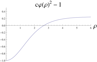
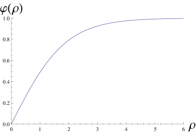
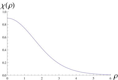
Figure 1: $b=1$, $c=1.25$, $\beta=8$

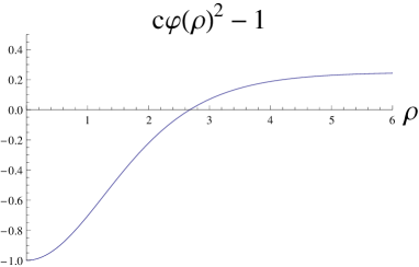
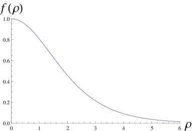
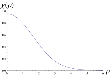
Figure 2: $b=2$, $c=1.25$, $\beta=16$

7 Conclusions

We discussed the theory supporting strings with extra (rotational) moduli on the string world sheet. Our numerical analysis demonstrates that it is not difficult to endow the ANO string with such moduli following a strategy similar to that used by Witten in constructing cosmic strings. Our discussion was carried out in the quasiclassical approximation.

When the bulk model is deformed by a spin-orbit interaction a number of entangled terms emerge on the string world sheet. Quantum effects on the string world sheet (which can be made arbitrarily small with a judicious choice of parameters) is a subject of a separate study.

References

- [1]
- [2] A. Abrikosov, Sov. Phys. JETP 32 1442 (1957); H. Nielsen and P. Olesen, Nucl. Phys. B61 45 (1973).
- [3] M. Shifman, Phys. Rev. D 87, 025025 (2013) [arXiv:1212.4823 [hep-th]].
- [4] M. Nitta, M. Shifman and W. Vinci, Phys. Rev. D 87, 081702 (2013) [arXiv:1301.3544 [cond-mat.other]].
- [5] M. Shifman, and A. Yung, Phys. Rev. Lett. 110, 201602 (2013) [arXiv:1303.7010 [hep-th]].
- [6] G. Volovik, The Universe in a Helium Droplet, (Oxford University Press, 2003); A. J. Leggett, Quantum Liquids (Oxford University Press, 2006).
- [7] E. A. Ivanov and V. I. Ogievetsky, Teor. Mat. Fiz. 25, 164 (1975) [English version in JINR Report JINR-E2-8593].
- [8] I. Low and A. V. Manohar, Phys. Rev. Lett. 88, 101602 (2002) [hep-th/0110285].
- [9] E. Witten, Nucl. Phys. B 249, 557 (1985).
- [10] M. Shifman, Advanced Topics in Quantum Field Theory, (Cambridge University Press, 2012).
- [11] E. B. Bogomol’nyi, Sov. J. Nucl. Phys. 24, 449 (1976), reprinted in Solitons and Particles, eds. C. Rebbi and G. Soliani (World Scientific, Singapore, 1984) p. 389. M. K. Prasad and C. M. Sommerfield, Phys. Rev. Lett. 35, 760 (1975), reprinted in Solitons and Particles, Eds. C. Rebbi and G. Soliani (World Scientific, Singapore, 1984) p. 530.
- [12]