The longitudinal response function of the deuteron in chiral effective field theory

Abstract

We use chiral effective field theory ($\chi$EFT) to make predictions for the longitudinal electromagnetic response function of the deuteron, $f_{L}$, which is measured in $d(e,e^{\prime}N)$ reactions. In this case the impulse approximation gives the full $\chi$EFT result up to corrections that are of $\mathcal{O}(P^{4})$ relative to leading order. By varying the cutoff in the $\chi$EFT calculation between 0.6 and 1 GeV we conclude that the calculation is accurate to better than 10% for values of $\mathbf{q}^{2}$ within 4 fm^-2 of the quasi-free peak, up to final-state energies $E_{np}=60$ MeV. In these regions $\chi$EFT is in reasonable agreement with predictions for $f_{L}$ obtained using the Bonn potential. We also find good agreement with existing experimental data on $f_{L}$, albeit in a more restricted kinematic domain.

I Introduction

The use of chiral perturbation theory ($\chi$PT) to describe few-nucleon systems is a problem that has received much attention over the past twenty years. This effort began with the seminal papers of Weinberg We90 , and has recently been reviewed in Refs. Ep08 ; Ep12 . In this approach the NN potential is computed up to some fixed order, $n$, in the chiral expansion in powers of $P\equiv(p,m_{\pi})/\Lambda_{0}$. Here $p$ is the NN c.m. momentum, $m_{\pi}$ the pion mass, and the breakdown scale $\Lambda_{0}$ is nominally $m_{\rho}\sim 4\pi f_{\pi}$, but in reality is somewhat lower for reactions involving baryons. This NN potential is then iterated, using the Schrödinger or Lippmann-Schwinger equation, to obtain the scattering amplitude. This approach has come to be known as chiral effective field theory ($\chi$EFT) as it encodes the consequences of QCD’s pattern of chiral-symmetry breaking for few-nucleon systems and is built on a systematic expansion in powers of $P$, while resumming the non-perturbative effects that lead to the existence of nuclear bound states.

Electromagnetic reactions provide particularly fertile ground for the application of $\chi$EFT. A few-nucleon electromagnetic current operator, $J_{\mu}$, can also be derived from $\chi$PT Ko09 ; Ko11 ; Pa08 ; Pa09 ; Pa11 ; Pi12 , and matrix elements are then constructed via:

$$\mathcal{M}_{\mu}=\langle\psi^{(f)}|\sum_{k=0}^{n}J_{\mu}^{(k)}|\psi^{(i)}\rangle,$$ (1)

where $|\psi^{(i)}\rangle$ and $|\psi^{(f)}\rangle$ are solutions of the Schrödinger equation for the $\chi$EFT potential $V$—in principle at order $n$. $\chi$PT predicts that short-distance effects will enter $J_{\mu}$ eventually, but minimal substitution generates the first several orders in the expansion for $J_{\mu}$, especially in the case of the charge operator. This enables predictions for charge form factors of $A=2$ PC99 ; WM01 ; Ph03 ; Ph07 ; Pi12 and $A=3$ Pi12 systems to be obtained as pure predictions up to order $P^{4}$ relative to leading order. These predictions agree well with data up to at least $Q^{2}=0.4$ GeV². In the magnetic response the first short-distance operator not determined by NN scattering or single-nucleon properties enters considerably earlier, but accurate predictions for form factors can still be made Ko12 ; Pi12 . Indeed, the existence of this additional short-distance operator allows enhanced understanding of magnetic moments and M1 transitions in systems up to $A=9$, with reactions that had not previously been understood now being explained, and correlated, through the presence of the same short-distance $\gamma$NN$\rightarrow$NN operator Gi10 ; Pa12 .

In this work we focus on the application of this formalism to electrodisintegration of deuterium, and specifically the computation of the longitudinal response function, $f_{L}$. $f_{L}$ is proportional to the square of the matrix element of the NN charge operator between the deuteron wave function and the wave function of a continuum NN state. $J_{0}$ is given solely by a single-nucleon operator up to $\mathcal{O}(P^{4})$ relative to leading order in the $\chi$EFT expansion, so calculations of $f_{L}$ can take the information gleaned on NN interactions from scattering experiments and use it to make quite accurate predictions for an electromagnetic observable. Deuteron electro-disintegration has been employed as a testing ground for NN models for a long time aren ; aren1 ; aren2 ; ALT00 ; ALT02 ; ALT05 . Since the 4-momentum in the breakup process is given by a virtual photon, a richer set of kinematics can be probed as compared to the photo-disintegration process. And, in addition to the deuteron wave function, the disintegration process probes both the on-shell and off-shell NN t-matrix through the final-state interaction.

This means that the solutions for the deuteron wave function $|\psi\rangle$, and the NN t-matrix, are input to our calculation. To obtain them from $\chi$EFT potentials we need to impose a cutoff on the intermediate states, $\Lambda$. The low-energy constants (LECs) multiplying contact interactions in the nucleon-nucleon part of the chiral Lagrangian should then be adjusted to eliminate any cutoff dependence $\sim\mathcal{O}(1)$ or greater in the effective theory’s predictions for low-energy observables. If this is not possible we conclude that $\chi$EFT is unable to give reliable predictions. At leading order the $\chi$EFT potential consists of a zero-derivative contact interaction that is operative only in NN partial waves with $L=0$ together with one-pion exchange, which is active in all partial waves. In an earlier work we showed how to “subtractively renormalize” the LO equations for NN scattering in these two channels Ya08 . This technique eliminates the contact interaction in favor of a low-energy observable (e.g. the relevant NN scattering length). This makes it straightforward to take the limit $\Lambda\rightarrow\infty$: no fine-tuning of the pertinent LEC is necessary. The resulting phase shifts (and one mixing parameter) do not provide anything like a precision description of NN data, but they are, at least, a well-defined, renormalized LO calculation.

However, several papers have demonstrated that a LO $\chi$EFT calculation does not produce reliable predictions in partial waves with $L>0$ once $\Lambda$ is sufficiently large ES03 ; NTvK05 ; Bi06 ; PVRA06 . This is because only one-pion exchange is present in these waves at LO, and the resulting singular potential has no NN LEC that permits renormalization. We examined this problem within the context of subtractive renormalization and confirmed the conclusion of Ref. NTvK05 , i.e. any partial wave with $L>0$ where one-pion exchange is attractive does not have stable LO results in $\chi$ET Ya09A . We also showed that this problem is not removed at $\mathcal{O}(P^{2})$ or $\mathcal{O}(P^{3})$. In particular, at $\mathcal{O}(P^{3})$ two-pion exchange produces a highly singular, attractive potential. The NN contact interactions needed to renormalize this potential are not present, e.g. in the ³P₂-³F₂ channel. The resulting lack of stability with $\Lambda$ of the NN phase shifts occurs once $\Lambda$ is larger than $\approx 1$ GeV. In Ref. Ya09B we used subtractive renormalization to calculate S-wave NN phase shifts from $\mathcal{O}(P^{2})$ and $\mathcal{O}(P^{3})$ $\chi$ET potentials. Here too we found that the phase shifts are not stable once $\Lambda>1$ GeV. In this case part of the problem is that the momentum-dependent contact interaction that appears at $\mathcal{O}(P^{2})$ has limited effect as $\Lambda\rightarrow\infty$ Wigner ; PC96 ; Sc96 . Thus the NN potential obtained by straightforward application of $\chi$PT cannot be used over a wide range of cutoffs: $\chi$EFT as formulated above is not properly renormalized, i.e. the impact of short-distance physics on the results is not under control.

Nevertheless, in Refs. Or96 ; Ep99 ; EM02 (Refs. EM03 ; Ep05 ) $V$ was computed to $\mathcal{O}(P^{2})$ and $\mathcal{O}(P^{3})$ ($\mathcal{O}(P^{4})$), and the several NN LECs which appear in $V$ were fitted to NN data for a range of cutoffs between 500 and 800 MeV. The $\mathcal{O}(P^{4})$ predictions contain very little residual cutoff dependence in this range of $\Lambda$’s, and describe NN data with considerable accuracy. This suggests that $\chi$EFT may be a systematic theory of few-nucleon systems if we employ $\Lambda$’s in the vicinity of $m_{\rho}$. Since the short-distance physics of the effective theory for $p\gg m_{\rho}$ is different to the short-distance physics of QCD itself, some authors argue that considering $\Lambda\gg m_{\rho}$ does not yield any extra information about the real impact of short-distance physics on observables Le97 ; EM06 . Using low cutoffs has the advantage that relevant momenta are demonstrably within the domain of validity of $\chi$PT. Discussion about whether such a procedure results in the omission of some operators is ongoing Bi09 ; Ph12 . In what follows we employ wave functions obtained with the standard $\chi$EFT counting and our subtractive renormalization method Ya09A ; Ya09B , but we do so only for cutoffs $\Lambda$ up to the maximum value where we found reasonable results in Refs. Ya09A ; Ya09B , i.e. $\Lambda\leq 1000$ MeV.

Our deuteron electrodisintegration calculation provides an opportunity to test this strategy, by comparing its predictions for deuteron structure and final-state interactions to experimental data. However, experimental data on $f_{L}$ are somewhat limited—especially in the low-energy and low-$\mathbf{q}^{2}$ region of most interest to $\chi$EFT. Much of the data on $f_{L}$ that do exist have been averaged over spectrometer acceptances, which makes comparison with theory not only complicated, but also, in some cases, ambiguous. Therefore, although we do compare with data from Refs. vdS91 ; Du94 ; Jo96 , we use the Bonn-potential calculations of Arenhövel et al. as a proxy for data. These calculations have been quite successful in describing data: non-L/T separated Be81 ; TC84 ; Br86 ; Bl98 , L/T-separated vdS91 ; Du94 ; Jo96 , and even on the interference response functions, $f_{LT}$ and $f_{TT}$ Ta87 ; vdS92 ; Fr94 ; Ka97 ; Zh01 ; Bo08 ; Re08 , taken at many different laboratories over a wide range of relevant kinematic conditions. (Note that we do not list data at squared momentum transfers $>1$ GeV² here because those are well outside the reach of $\chi$EFT, and even beyond the scope of the semi-relativistic treatment of Arenhövel et al.. For recent progress on high-$Q^{2}$ electrodisintegration see Refs. Ul02 ; Bo11 ; JvO08 ; JvO10 and references therein.)

A necessary condition for the $\chi$EFT predictions to be considered reliable is that they show minimal dependence on the cutoff $\Lambda$. We will use this criterion to diagnose situations in which the final-state interaction matrix-element computation has significant sensitivity to short-distance physics. Deuteron photodisintegration has been studied (albeit with an incomplete current operator) in $\chi$EFT by Rozdzepik et al. using a similar strategy and the wave functions of Refs. Ep05  Ro11 . Since this process involves real photons, it is sensitive to the deuteron transverse response function, $f_{T}$, and has no dependence on the response function computed here. Christlmeier and Grießhammer computed deuteron electrodisintegration at very low energies and momentum transfers in the pionless effective field theory CG08 . They demonstrated the incompatibility of the data on the mixed response function $f_{LT}$, published by von Neumann-Cosel et al. with the low-energy NN phase-shift data and our knowledge of other electromagnetic transitions in the NN system vNC02 . This helped them diagnose a flaw in the analysis of Ref. vNC02 . Pionless EFT was also successfully applied to the $(e,e^{\prime})$ data taken in a later experiment at S-DALINAC Re08 .

The paper is structured as follows. In Sec. II we review the facts about the NN charge operator which are relevant for our study. In Sec. III, we introduce the general set up of the electrodisintegration problem and lay out the basic formulae. In Sec. IV we evaluate the matrix element of $J_{0}$ which enters $f_{L}$ and derive an explicit expression for it in terms of partial waves. We also present the NN input used, i.e. results for deuteron wave functions and NN phase shifts from Refs. Ya09A ; Ya09B . In Section V we present our results for the longitudinal response function. We pay particular attention to the kinematic regions where significant dependence of $f_{L}$ on the momentum cutoff $\Lambda$ is and is not present. We present our conclusions in Sec. VI.

II The NN charge operator to $\mathcal{O}(eP^{3})$

In this section we analyze the NN charge operator $J_{0}$, expanding it in powers of the $\chi$EFT small parameter $P$. Since our wave functions are computed up to $\mathcal{O}(P^{3})$ relative to leading order, we also need the two-nucleon charge operator $J_{0}$ up to the same relative accuracy. We denote the leading order for $J_{0}$ as $\mathcal{O}(e)$. A $J_{0}$ that is consistent with chiral potential $V$ up to $\mathcal{O}(eP^{4})$ (and obeys appropriate Ward identities) has recently been obtained by several authors Ko09 ; Ko11 ; Pa09 ; Pa11 ; Pi12 . We now summarize the results needed for this study.

The analysis proceeds by dividing the charge operator into an isoscalar part $J_{0}^{(s)}$, and an isovector one $J_{0}^{(v)}$. Up to corrections of $\mathcal{O}(eP^{4})$ in the chiral expansion we have, on the basis of states of NN relative momentum :

$$\langle\mathbf{p}^{\prime}|J_{0}^{(s)}(\mathbf{q})|\mathbf{p}\rangle=\left[\delta(\mathbf{p}^{\prime}-\mathbf{p}-\mathbf{q/2})+\delta(\mathbf{p}^{\prime}-\mathbf{p}+\mathbf{q/2})\right]G_{E}^{(s)}(Q^{2})$$ (2)

where $G_{E}^{(s)}$ is the isoscalar nucleon form factor, and we have summed over the contributions of nucleons one and two. In the case of the deuteron we may use the symmetry of the state (only even partial waves are present) to prove that the two terms in square brackets are equal.

Meanwhile for $J_{0}^{(v)}$ we have:

$$\langle\mathbf{p}^{\prime}|J_{0}^{(v)}(\mathbf{q})|\mathbf{p}\rangle=\left[\delta(\mathbf{p}^{\prime}-\mathbf{p}-\mathbf{q}/2)\tau_{3}^{(1)}+\delta(\mathbf{p}^{\prime}-\mathbf{p}+\mathbf{q}/2)\tau_{3}^{(2)}\right]G_{E}^{(v)}(Q^{2}),$$ (3)

where $G_{E}^{(v)}$ is the isovector nucleon form factor. This operator does not contribute to the matrix elements for elastic scattering, but it is relevant for electrodisintegration. $G_{E}^{(s)}$ and $G_{E}^{(v)}$ are related to the proton (neutron) charge form factor $G_{E}^{(p)}$ ($G_{E}^{(n)}$) by

$$G_{E}^{(s,v)}(Q^{2})=\frac{1}{2}(G_{E}^{(p)}(Q^{2})\pm G_{E}^{(n)}(Q^{2})),$$ (4)

where the $+(-)$ sign applies to the $s(v)$ case.

$\chi$PT does a reasonable job describing $G_{E}^{(v)}$ for squared 4-momentum $Q^{2}<0.1$ GeV², but its description of isoscalar nucleon structure $G_{E}^{(s)}$ is of limited utility, even in this low-$Q^{2}$ domain Be92 ; Ph09 . Our goal here is to look at higher $|\mathbf{q}|$, and we do not wish to be limited in our pursuit of that goal by $\chi$PT’s description of single-nucleon electromagnetic structure.

There are no two-body corrections to $J_{0}$ at $\mathcal{O}(eP^{2})$. It might seem that there will be an effect in $J_{0}^{(v)}$, because the $A_{0}$ photon can couple directly to the exchanged pion. However, in the static limit used to obtain NN potentials and charge operators that pion line carries no energy. Thus two-body corrections to $J_{0}^{(v)}$ that contain such an effect are deferred until $\mathcal{O}(eP^{4})$, because we follow the counting of Ref. Ep05 and count $p/M\sim\mathcal{O}(P^{2})$ while $p/\Lambda\sim\mathcal{O}(P)$. At $\mathcal{O}(eP^{3})$ an NN contribution to $J_{0}$ must be built out of a vertex from $\mathcal{L}_{\pi N}^{(2)}$, one from $\mathcal{L}_{\pi N}^{(1)}$ and a pion propagator. However, the only term in $\mathcal{L}_{\pi N}^{(2)}$ that couples an $A_{0}$ photon to a nucleon and a pion has a fixed $1/M$ coefficient, so this effect is also deferred until $\mathcal{O}(eP^{4})$.

Therefore, in the counting where $p/M\sim P^{2}$, the NN charge operator is given by Eqs. (2) and (3), up to corrections of $\mathcal{O}(eP^{4})$.

III Basic formulae for deuteron electrodisintegration

The usual expression for the differential cross section for deuteron electro-disintegration is (see, for example, Ref. aren1 )

$$\frac{d^{3}\sigma}{dk_{2}^{lab}d\Omega_{e}^{lab}d\Omega_{p}}=c\{\rho_{L}f_{L}+\rho_{T}f_{T}+\rho_{LT}f_{LT}\cos[\phi]+\rho_{TT}f_{TT}\cos[2\phi]\}.$$ (5)

$\rho(f)_{L,T,LT,TT}$ describe the lepton (hadron) tensor. The kinematics is to be visualized as in Fig. 1. Here the virtual photon gives its 4-momentum ($\omega,\mathbf{q}$) to the deuteron, with these quantities determined by the initial electron energy and $\theta_{e}$, the electron scattering angle. $\theta$ is the angle between $\mathbf{q}$ and the momentum $\mathbf{p}^{\prime}$ of the outgoing proton. (Here and in what follows, unless otherwise stated, we work in the c.m. frame of the final proton-neutron pair. If necessary, the superscript “lab” is used to denote quantities in the lab. frame.) Meanwhile, $\phi$ is the angle between the scattering plane containing the two electron momentum vectors and the plane formed by the outgoing proton and neutron. Finally, in Fig. 1 we have defined $\mathbf{q}$ to be along the z-axis. Hence $\Omega_{e}^{lab}=(\theta_{e}^{lab},\phi_{e}^{lab}),$ $\Omega_{p}=(\theta,\phi)$. Meanwhile,

$$c=\frac{\alpha}{6\pi^{2}}\frac{k_{2}^{lab}}{k_{1}^{lab}(q^{2})^{2}},$$ (6)

where $\alpha$ is the fine structure constant, $k_{1(2)}^{lab}$ is the absolute value of the incoming (outgoing) electron 3-momentum in the laboratory frame, and $q^{2}$ is the 4-momentum-squared of the virtual photon.

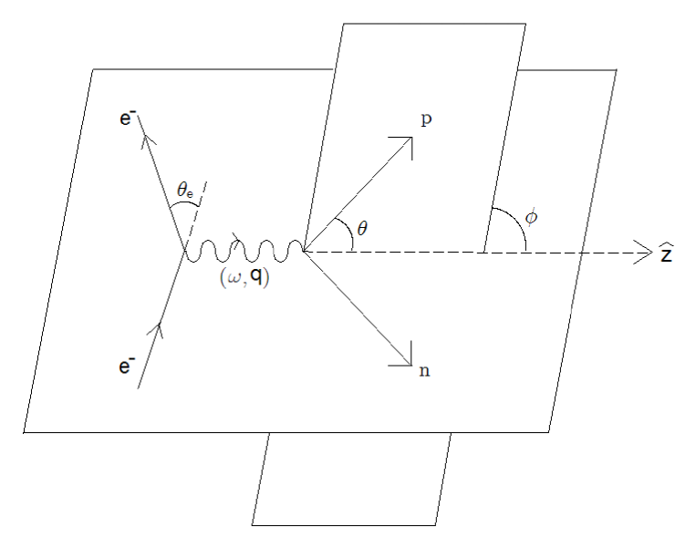
Figure 1: The kinematic description of the deuteron electro-disintegration process. The labels are specified in the text below.

In the (final-state) c.m. frame we have

proton (neutron) 3-momentum $$: \mathbf{p}^{\prime}\mathbf{(-p}^{\prime}\mathbf{),}$$

proton (neutron) total energy $$: E_{n}=E_{p}=M+\frac{\mathbf{p}^{\prime 2}}{2M},$$

total energy of deuteron $$: E_{d}=M_{d}+\frac{\mathbf{q}^{2}}{2M_{d}},\text{ }M_{d}=2M-B.$$ (7)

Here $M(M_{d})$ represents the rest mass of the nucleon (deuteron) and $B=2.24$ MeV is the deuteron binding energy. From energy conservation: $|\mathbf{p}^{\prime}|=\sqrt{(\omega-B)M+(\mathbf{q})^{2}\frac{M}{2M_{d}}}$. The quantities in the lab. frame can be easily related to those in c.m. frame by a Lorentz boost CG08 by an amount

$$\beta=\frac{|\mathbf{q|}^{lab}}{M_{d}+\omega^{lab}},$$ (8)

i.e.,

$$\omega^{cm} = \gamma\omega^{lab}-\beta\gamma|\mathbf{q|}^{lab},$$

$$|\mathbf{q|}^{cm} = \beta\gamma M_{d}.$$ (9)

For this work, we do not consider the electron polarization degree of freedom, and calculate only the contribution from the longitudinal part in Eq. (5), which is thus rewritten as

$$\frac{d^{3}\sigma_{longitudinal}}{dk_{2}^{lab}d\Omega_{e}^{lab}d\Omega_{p}}=\frac{\alpha}{2\pi^{2}}\frac{k_{2}^{lab}}{k_{1}^{lab}(q^{2})^{2}}\sum\limits_{SM_{s}m_{J}}\rho_{L}T_{SM_{s}0m_{J}}T_{SM_{s}0m_{J}}^{\ast},$$ (10)

where the lepton tensor

$$\rho_{L}=4E_{e}^{lab}E_{e}^{\prime lab}(\frac{q^{2}}{\mathbf{q}^{2}})\cos^{2}\left(\frac{\theta_{e}^{lab}}{2}\right),$$ (11)

and $T_{SM_{s}\mu m_{J}}$ is defined as aren :

$$T_{SM_{s}\mu m_{ds}}=-\pi\sqrt{2\alpha|\mathbf{p}^{\prime}|E_{p}E_{d}/M_{d}}\langle\Psi_{\mathbf{p}^{\prime}SM_{s}}|J_{\mu}(\mathbf{q})|m_{J}\rangle.$$ (12)

In Eq. (12) $\langle\Psi_{\mathbf{p}^{\prime}SM_{s}}|$ is the NN final state with the total spin quantum number $S$ and its projection on the z-axis, $M_{s}$, both specified, $\mathbf{p}^{\prime}$ represents that the final proton has 3-momentum $\mathbf{p}^{\prime}$, and $\mu$ labels the polarization index of the virtual photon. We consider only $\mu=0$ here. The deuteron state $|m_{J}\rangle$ has total angular momentum 1, and $m_{J}$ labels the z-projection of its total angular momentum. The angular dependence of Eq. (12) can be separated into two parts, i.e.,

$$T_{SM_{s}\mu m_{J}}(\theta,\phi)=e^{i(\mu+m_{J})\phi}x_{SM_{s}\mu m_{J}}(\theta).$$ (13)

The longitudinal structure function $f_{L}$ is obtained from the $\theta$-dependent part of $T_{SM_{s}0m_{J}}$, i.e.,

$$f_{L}=\sum\limits_{SM_{s}m_{J}}x_{SM_{s}0m_{J}}x_{SM_{s}0m_{J}}^{\ast},$$ (14)

and so $\frac{d^{3}\sigma_{longitudinal}}{dk_{2}^{lab}d\Omega_{e}^{lab}d\Omega_{p}}\sim f_{L}$, with the proportionality determined solely by kinematic factors.

IV Evaluating the matrix element

From Eqs. (12) and (14), one sees that to obtain $f_{L},$ the matrix element $\langle\Psi_{\mathbf{p}^{\prime}SM_{s}}|J_{0}(\mathbf{q})|m_{J}0\rangle$ needs to be evaluated, which, up to $\mathcal{O}(eP^{4})$, can be represented by

$$\langle\Psi_{\mathbf{p}^{\prime}SM_{s}T}|J_{0}(\mathbf{q})|m_{J}0\rangle = \langle\mathbf{p}^{\prime}SM_{s}T|J_{0}(\mathbf{q})|m_{J}0\rangle$$ (15)

$$+\langle\mathbf{p}^{\prime}SM_{s}T|t(E^{\prime})G_{0}(E^{\prime})J_{0}(\mathbf{q})|m_{J}0\rangle,$$

with $J_{0}$ given by Eqs. (2) and (3), and $t(E^{\prime})$ and $G_{0}(E^{\prime})$ the NN t-matrix and free Green’s function. Here we have used the $T$ to represent the fact that the final-state wavefunction is isospin dependent and introduced a $0$ in the kets and the $T$ in the two bras on the right-hand side to indicate the isospin of those states.

The first term on the right-hand side of Eq. (15) is the plane-wave impulse approximation (PWIA), and the second term is the final-state interaction (FSI). The dynamics of the PWIA part can be described by Fig. 2: there the final-state proton (neutron) has 3-momentum $\mathbf{p}^{\prime}(-\mathbf{p}^{\prime})$ in the final c.m. frame, while before the proton (neutron) is struck, it has 3-momentum $\mathbf{p}^{\prime}-\mathbf{q}/2$ $(-\mathbf{p}^{\prime}-\mathbf{q}/2)$ in the deuteron’s c.m. frame.

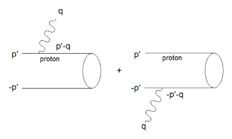
Figure 2: The plane-wave impulse approximation diagrams for deuteron electro-disintegration. The blob on the right of each diagram represents the deuteron state. All momenta in the figure are measured in the final proton-neutron c.m. frame.

IV.1 Isospin decomposition

By inserting a complete set of isospin states and using the identity:

$$\langle\mathbf{p}SM_{s}TM_{T}|G_{0}(E^{\prime})|\mathbf{p}^{\prime\prime}S^{\prime\prime}M_{s}^{\prime\prime}T^{\prime\prime}M_{T}^{\prime\prime}\rangle = \delta(\mathbf{p}-\mathbf{p}^{\prime\prime})\delta_{SS^{\prime\prime}}\delta_{M_{s}M_{s}^{\prime\prime}}\delta_{TT^{\prime\prime}}\delta_{M_{T}M_{T}^{\prime\prime}}$$ (16)

$$\times\left[\frac{{\mathcal{P}}}{E^{\prime}-\mathbf{p}^{2}/M}-i\pi\delta\left(E^{\prime}-\mathbf{p}^{2}/M\right)\right].$$

we obtain

$${\langle\mathbf{p}^{\prime}SM_{s}\Psi_{T}|t(E^{\prime})G_{0}(E^{\prime})J_{0}(\mathbf{q})|m_{J}0\rangle}=\sum_{T=0,1}\int d^{3}p\,\langle\mathbf{p}^{\prime}SM_{s}T|t(E^{\prime})|\mathbf{p}SM_{s}T\rangle$$

$$\times\left[\frac{{\mathcal{P}}}{E^{\prime}-\mathbf{p}^{2}/M}-i\pi\delta\left(E^{\prime}-\frac{\mathbf{p}^{2}}{M}\right)\right]\langle\mathbf{p}SM_{s}T|J_{0}(\mathbf{q})|m_{J}0\rangle,$$ (17)

with $E^{\prime}=\frac{\mathbf{p^{\prime}}^{2}}{M},$ and ${\mathcal{P}}$ denotes the principal value. Note that in Eq. (15) the magnitude of $\mathbf{p}^{\prime}$ is restricted to be that of the proton in the final-state c.m. frame, while in Eq. (17) $\mathbf{p}$ is the integration variable. Note also that in Eq. (17), and in what follows, we have dropped the $M_{T}$ label, since all states have $M_{T}=0$: there are no interactions present that change this quantum number.

The matrix element $\langle\mathbf{p^{(\prime)}}SM_{s}T|J_{0}(\mathbf{q})|m_{J}0\rangle$ needs to be evaluated so that we can calculate Eq. (15). The matrix element can be evaluated as

$$\langle\mathbf{p}SM_{s}T|J_{0}(\mathbf{q})|m_{J}0\rangle=\sum_{i=1,2}\langle\mathbf{p}_{i}-\frac{\mathbf{q}}{2}SM_{s}|m_{J}\rangle(\delta_{T0}G_{E}^{s}(\mathbf{q}^{2})\pm\delta_{T1}G_{E}^{v}(\mathbf{q}^{2})),$$ (18)

where the $+(-)$ sign applies to the $i=1(2)$ case, and the second factor on each line is now purely a matrix element in isospin space. Here $\mathbf{p}_{1(2)}$ is the momentum of particle 1(2) in the final c.m. frame. Note that particle 1(2) can be either a proton or neutron.

Substituting

Eqs. (4) and (18) into Eq. (15) and Eq. (17), we get the final expression

$$\langle\mathbf{p}^{\prime}SM_{s}\Psi_{T}|(1+tG_{0})J_{0}(\mathbf{q})|m_{J}0\rangle$$ (19)

$$= \langle\mathbf{p}^{\prime}-\frac{\mathbf{q}}{2}\;SM_{s}|m_{J}\rangle G_{E}^{(p)}(\mathbf{q}^{2})+\langle-\mathbf{p}^{\prime}-\frac{\mathbf{q}}{2}\;SM_{s}|m_{J}\rangle G_{E}^{(n)}(\mathbf{q}^{2})$$

$$+\frac{1}{2}\sum_{T=0,1}\int d^{3}p\,\langle\mathbf{p}^{\prime}SM_{s}T|t|\mathbf{p}SM_{s}T\rangle\left[\frac{{\mathcal{P}}}{E^{\prime}-\mathbf{p}^{2}/M}-i\pi\delta(E^{\prime}-\mathbf{p}^{2}/M)\right]$$

$$\quad\times\left[\langle\mathbf{p}-\frac{\mathbf{q}}{2}SM_{s}|m_{J}\rangle+(-1)^{T}\langle-\mathbf{p}-\frac{\mathbf{q}}{2}SM_{s}|m_{J}\rangle\right](G_{E}^{(p)}(\mathbf{q}^{2})+(-1)^{T}G_{E}^{(n)}(\mathbf{q}^{2})).$$

Note that the final-state interaction piece in Eq. (19) itself has two parts: one for $T=0$ and one for $T=1$. Each part consists of a t-matrix, the free Green’s function and the deuteron wave function with the nucleon form factors. Here we need to integrate over $\mathbf{p}$, thus the deuteron wave function is multiplied by the half-shell t-matrix $t$($\mathbf{p}^{\prime}\mathbf{,p};E_{np}$). In principle, arbitrarily high values of $|\mathbf{p}|$ contribute to the integration which yields the electrodisintegration amplitude. Physically, this means that the virtual photon can strike one of the nucleons in a state with arbitrarily large 3-momentum $-\mathbf{q}+\mathbf{p}$ (the other nucleon will have momentum $-\mathbf{p}$ in the final proton-neutron c.m. frame). The two nucleons then exchange momentum to reach their final state through the FSI. This is in contrast with the PWIA, where, to reach a given final state, the virtual photon must strike the nucleon at a specific momentum. However, in practice, the high-$|\mathbf{p}|$ component of the deuteron wave function is small, so the high-momentum part of the FSI integral will be suppressed.

At this point, we have an expression for the sum of a plane-wave-impulse-approximation piece and the final-state interaction in terms of the 3-momentum of the measured proton $\mathbf{p}^{\prime}$. The next step is to express Eq. (19) in terms of partial waves.

IV.2 Partial-wave decomposition

IV.2.1 Plane-wave impulse approximation

First, we perform the partial-wave decomposition of the PWIA part of Eq. (19). To do this we insert

$$1=\frac{2}{\pi}\sum_{\begin{subarray}{c}J,m_{J},LS\\ with|L-S|\leq J\leq|L+S|\end{subarray}}\int\limits_{0}^{\infty}dp\,p^{2}|pJm_{J}LS\rangle\langle pJm_{J}LS|$$ (20)

into $\langle\mathbf{p}^{\prime}-\frac{\mathbf{q}}{2}SM_{s}|m_{J}\rangle$, where $p=|\mathbf{p}|$. Note that the normalization adopted here is

$$\langle\mathbf{k}^{\prime}|\mathbf{k}\rangle=\delta(\mathbf{k}-\mathbf{k}^{\prime})$$ (21)

and hence

$$\langle p^{\prime}J^{\prime}m_{J^{\prime}}L^{\prime}S^{\prime}|pJm_{J}LS\rangle=\frac{\pi}{2}\frac{\delta(p-p^{\prime})}{p^{2}}\delta_{JJ^{\prime}}\delta_{m_{J}m_{J^{\prime}}}\delta_{L^{\prime}L}\delta_{S^{\prime}S}.$$ (22)

Meanwhile, the deuteron wave function appears as matrix elements

$$\langle|\mathbf{p}^{\prime}-\frac{\mathbf{q}}{2}\mathbf{|}\,Jm_{J}LS|m_{J}\rangle=i^{L}\Psi_{L}\left(|\mathbf{p}^{\prime}-\frac{\mathbf{q}}{2}\mathbf{|}\right),$$ (23)

where the S- ($L=0$) and D- ($L=2$) wave components of the deuteron wave function satisfy

$$\frac{2}{\pi}\int dpp^{2}[\Psi_{0}^{2}(p)+\Psi_{2}^{2}(p)]=1.$$ (24)

The momentum-space wave functions we employ are obtained using the methods discussed in ref.Ya08 , and are shown, together with those of the CD-Bonn potential, in Fig. 3.

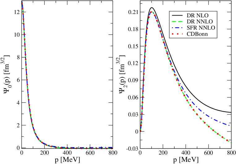
Figure 3: The momentum-space wave functions of the deuteron as a function of p, where $\psi_{0}$(p) is the ³S₁ wave function and $\psi_{2}$(p) denotes the ³D₁ wave function. These wave functions are obtained from the dimensional-regularization (DR) two-pion-exchange potential (TPE) up to next-to leading order (NLO), i.e., $\mathcal{O}(Q^{2})$ (black solid line), DR TPE up to next-to-next-to leading order (NNLO), i.e., $\mathcal{O}(Q^{3})$ (green dashed line), and the spectral-function-regularization (SFR) TPE up to NNLO (blue dash-dotted line), where the cutoff in the Lippmann-Schwinger equation (LSE) is $\Lambda=800$ MeV, and the SFR intrinsic cutoff is $\widetilde{\Lambda}=800$ MeV. The red dots indicate the corresponding wave functions obtained from the CD-Bonn potential.

Putting this all together and using the plane-wave expansion formula (with S=1 for deuteron)

$$|\mathbf{p}^{\prime}1M_{s}\rangle=\sqrt{\frac{2}{\pi}}\sum_{L^{\prime},m_{l}^{\prime}}Y_{L^{\prime}m_{l}^{\prime}}^{\ast}(\Omega_{p^{\prime}})|p^{\prime}L^{\prime}m_{l}^{\prime}\rangle\otimes|1M_{s}\rangle,$$ (25)

the two contributions to the PWIA matrix element become:

$$\langle\pm\mathbf{p}^{\prime}-\frac{\mathbf{q}}{2}\;1M_{s}|m_{J}\rangle = \sqrt{\frac{2}{\pi}}\sum_{L=0,2}\sum_{m_{l}}(Lm_{l}1M_{s}|1m_{J})Y_{Lm_{l}}(\Omega_{\pm p^{\prime}-q/2})i^{L}\Psi_{L}\left(\mathbf{|}\mathbf{p}^{\prime}\mp\frac{\mathbf{q}}{2}\mathbf{|}\right).$$

Here $(Lm_{l}1M_{s}|1m_{J})$ is the Clebsch-Gordan coefficient and $\Omega_{\pm p^{\prime}-q/2}$ is the angle between $\widehat{z}$ and $\pm\mathbf{p}^{\prime}-\frac{\mathbf{q}}{2}$.

IV.2.2 Final-state interaction

One can follow the same logic as for the PWIA piece to perform the partial-wave decomposition of the FSI term. Note that the total spin ($S$) and isospin ($T$) are conserved in the NN interaction. Thus

$$\langle\mathbf{p}^{\prime}SM_{s}T|t(E^{\prime})G_{0}(E^{\prime})J_{0}(\mathbf{q})|m_{J}0\rangle$$

$$=\sum_{M_{s}^{\prime}}\int d^{3}p\langle\mathbf{p}^{\prime}SM_{s}T|t(E^{\prime})|\mathbf{p}SM_{s}^{\prime}T\rangle\left[\frac{{\mathcal{P}}}{E^{\prime}-\mathbf{p}^{2}/M}-i\pi\delta\left(E^{\prime}-\frac{\mathbf{p}^{2}}{M}\right)\right]\langle\mathbf{p}SM_{s}^{\prime}T|J_{0}(\mathbf{q})|m_{J}0\rangle.$$

The matrix element $\langle\mathbf{p}S^{\prime}M_{s}^{\prime}T|J_{0}(\mathbf{q})|m_{J}0\rangle$ is evaluated via the first line of Eq. (19) and Eq. (IV.2.1). The 3-dimensional t-matrix $t(\mathbf{p}^{\prime},\mathbf{p};E^{\prime})$ can be constructed from $t_{LSJ}(p^{\prime},p;E)$. Since the deuteron has $S=1$, we need only $t_{L1J}(p^{\prime},p;E)$, for which:

$$\langle\mathbf{p}^{\prime}1M_{s}T_{f}|t(E^{\prime})|\mathbf{p}1M_{s}^{\prime}T_{f}\rangle$$

$$\qquad=\frac{2}{\pi}\sum_{{}_{\begin{subarray}{c}J,m_{j},L,L^{\prime\prime}\\ m_{l}m_{l}^{\prime\prime}\end{subarray}}}(Lm_{l}1M_{s}|Jm_{j})Y_{Lm_{l}}(\Omega_{p^{\prime}})t_{L1J,T_{f}}(E^{\prime})(L^{\prime\prime}m_{l}^{\prime\prime}1M_{s}^{\prime}|Jm_{j})Y_{L^{\prime\prime}m_{l}^{\prime\prime}}^{\ast}(\Omega_{p}).$$ (28)

Upon insertion of these results into Eq. (IV.2.2) we find that we need to perform the angular part of the integral in the following form

$$\int Y_{L^{\prime\prime}m_{l}^{\prime\prime}}^{\ast}(\Omega_{p})Y_{Lm_{l}}(\Omega_{\pm p-q/2})d\Omega_{p}.$$ (29)

Here $\Omega_{\pm p-q/2}$ is the solid angle between $\widehat{z}$ and $\pm\mathbf{p-q/}2$. We now denote the angle between $\widehat{z}$ and $\mathbf{p-q/}2$ as ($\theta^{\prime},\phi$), and

$$\theta^{\prime}=\sin^{-1}\left[\frac{|\mathbf{p}|\sin\theta}{\sqrt{|\mathbf{p}|^{2}-|\mathbf{p}||\mathbf{q}|\cos\theta+|\mathbf{q}|^{2}/4}}\right],$$ (30)

with $(\theta,\phi)$ the solid angle between $\mathbf{p}^{\prime}$ and $\hat{z}$. Similarly, the angle between $\widehat{z}$ and $-\mathbf{p-q/}2$, which we denote as ($\theta^{\prime\prime},\phi+\pi$), is

$$\theta^{\prime\prime}=\sin^{-1}\left[\frac{|\mathbf{p}|\sin\theta}{\sqrt{|\mathbf{p}|^{2}+|\mathbf{p}||\mathbf{q}|\cos\theta+|\mathbf{q}|^{2}/4}}\right].$$ (31)

Thus, to evaluate $\langle\mathbf{p}^{\prime}S=1M_{s}T_{f}|t(E^{\prime})G_{0}(E^{\prime})J_{0}(\mathbf{q})|m_{J}0\rangle,$ we need to do the integral over the angles $\theta$ and $\phi$. The integral over $\phi$ can be reduced by taking advantage of the property of spherical harmonics:

$$\int_{0}^{2\pi}\int_{0}^{\pi}Y_{lm}^{\ast}(\theta,\phi)Y_{l^{\prime}m^{\prime}}(\theta^{\prime},\phi)d(\cos\theta)d\phi$$ (32)

$$= 2\pi\delta_{mm^{\prime}}\sqrt{\frac{2l+1}{4\pi}\frac{(l-m)!}{(l+m)!}\frac{2l^{\prime}+1}{4\pi}\frac{(l^{\prime}-m)!}{(l^{\prime}+m)!}}\int_{0}^{\pi}P_{l}^{m}(\cos\theta)P_{l^{\prime}}^{m}(\cos\theta^{\prime})d(\cos\theta).$$

With the aid of Eq. (32), we can then perform the numerical integration over $\theta$ and $p$ to obtain the final-state interaction contribution to the longitudinal response function.

In doing this it is clearly important to have a description of the NN interaction that agrees with data for NN final-state energies of interest. In fact, the LECs of the NN t-matrix we adopted in our calculation of $f_{L}$ are those which generate phase shifts that agree with the Nijmegen phase-shift analysis nnonline ; St93 for $T_{lab}\leq 100$ MeV (as can be seen in Figs. 4 and 5). This kinematics corresponds to $E_{np}\leq 50$ MeV.

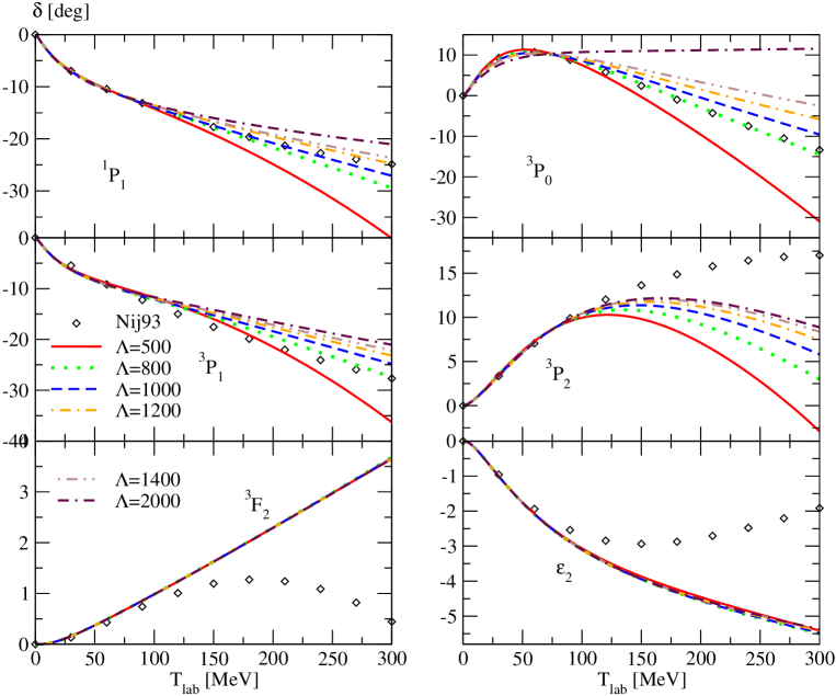
Figure 4: The NN P-wave phase shifts as a function of the laboratory kinetic energy that result from choosing $v^{LR}=v_{1\pi}+v_{2\pi}$, with the latter chosen to be the SFR TPE up to NNLO (with intrinsic cutoff $\widetilde{\Lambda}=800$ MeV). Here the generalized scattering lengths $\alpha_{11}^{SJ}$ are adjusted to give the best fit in the region $T_{lab}<100$ MeV. The Nijmegen phase-shift analysis  nnonline ; St93 is indicated by the open diamonds. This graph is adapted from our previous publication Ya09A .

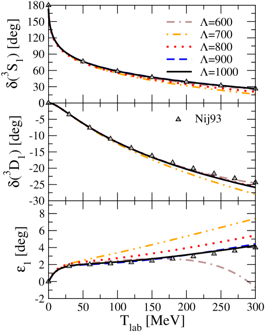
Figure 5: The best fit for the NN ³S${}_{1}-^{3}$D₁ phase shifts as a function of the laboratory kinetic energy for different cutoffs $\Lambda$ ranging from 0.6 to 1 GeV. The potentials employed are the SFR NNLO (with intrinsic cutoff $\widetilde{\Lambda}=800$ MeV). The values of the Nijmegen phase-shifts  nnonline ; St93 are indicated by the open triangles.

V Results for the longitudinal response function

In this section we present our results for the longitudinal response function of deuteron electro-disintegration. For the nucleon form factors we adopt the results listed in Ref. Bel . For electro-disintegration, one needs to specify two kinematic variables, e.g., ($\omega,\mathbf{q}$) to describe the whole process. We adopted the following kinematic variables in order to compare our results with those obtained with the Bonn potential in Ref. aren : first, the final energy of the proton-neutron system, which hereafter is labeled $E_{np},$ (previously it was denoted $E^{\prime}$) i.e.,

$$E_{np}=\frac{\mathbf{p}^{\prime 2}}{M};$$ (33)

second, the 3-momentum of the virtual photon (also in the system’s final c.m. frame) $\mathbf{q}_{cm}^{2}$. With $E_{np}$ and $\mathbf{q}_{cm}^{2}$ specified, the energy of the virtual photon can be calculated to be

$$\omega_{cm}=E_{np}-\sqrt{M_{d}^{2}+\mathbf{q}_{cm}^{2}}+2M.$$ (34)

The experimental data of Refs. vdS91 ; Du94 ; Jo96 are presented in terms of the lab. frame value of $|\mathbf{q}|$ and the value of the “missing momentum”,

$$\mathbf{p}_{m}=\mathbf{p}^{\prime}_{lab}-\mathbf{q}_{lab},$$ (35)

with $\mathbf{p}_{lab}^{\prime}$ the momentum of the detected proton. All these data were taken in kinematics such that $\mathbf{p}_{lab}^{\prime}$ and $\mathbf{q}_{lab}$ are aligned, and so $\theta=\phi=0$. From this information, and knowledge of the virtual-photon energy, $\omega_{lab}$, we can compute the kinetic energy of the np pair in the lab frame in two different ways:

$$E_{np,lab}=\omega_{lab}+M_{d}-2M=\sqrt{M^{2}+\mathbf{p}_{m}^{2}}+\sqrt{M^{2}+\mathbf{p}^{\prime 2}}-2M.$$ (36)

Lorentz transformation of this quantity to the cm frame according to

$$E_{np,cm}=\gamma(E_{np,lab}-\beta|\mathbf{{q}|),}$$ (37)

with $\beta$ given by Eq. (8), yields the $E_{np}$ which we quote in our results. Alternatively, $E_{np,cm}$ can be obtained by energy conservation, applied in the cm frame:

$$E_{np,cm}=\sqrt{M_{d}^{2}+\mathbf{q}_{cm}^{2}}+\omega_{cm}-2M$$ (38)

where $\omega_{cm}$ and $\mathbf{q}_{cm}$ are obtained from $\omega_{lab}$ and $\mathbf{q}_{lab}$ using Eq. (9).

Before presenting the results, we introduce one kinematics which is of particular interest: the so-called quasi-free ridge. The quasi-free ridge occurs when $\omega_{cm}=0$. Physically, this means that the virtual photon hits one of the nucleons and gives just enough 3-momentum to put it on-mass-shell. The other nucleon remains at rest in the laboratory frame. This occurs when:

$$E_{np,cm}\approx M_{d}(1+\frac{\mathbf{q}_{cm}^{2}}{2M_{d}^{2}})-2M\approx\frac{\mathbf{q}_{cm}^{2}}{2M_{d}}.$$ (39)

Consequently, on the quasi-free ridge $E_{np}$ (in MeV)$\approx 10\,\mathbf{q}_{cm}^{2}$ (in fm^-2).

We now present our results. First, we adopt the NN t-matrix and deuteron wave function generated with spectral-function regularization (SFR) applied to the two-pion-exchange potential up to NNLO, with the SFR cutoff $\widetilde{\Lambda}$ set to $800$ MeV. Fig. 6 shows the longitudinal structure function $f_{L}$ versus angle $\theta$, i.e., the angle between $\mathbf{p}^{\prime}$ and $\mathbf{q,}$ for $E_{np}=10$ MeV and $\mathbf{q}_{cm}^{2}=0.25-25$ fm^-2. The $\chi$EFT PWIA result is denoted by the red dash-double-dotted line, with error bars indicating the effect of varying the cutoff in the Lippmann-Schwinger equation (LSE) from $\Lambda=600-1000$ MeV. It is obtained using the full deuteron wave function obtained from the SFR TPE potential, evaluated at the pertinent three-momentum, see Eq. (IV.2.1).

For the final-state interaction (FSI), one needs to sum over partial-waves in order to obtain the 3-dimensional t-matrix. We have summed over partial-waves up to $J=3,$ and the results are denoted as blue dashed ($J=1$), green dash-dotted ($J$ up to $2$) and black double-dash-dotted ($J$ up to $3$) line in Fig. 6. In general, our results converge once we include partial waves with $J=2$ in our calculation of the FSI.

Here and below we compare our calculations to the calculations of Arenhövel and collaborators aren ; Aren10 . These calculations are done using the Bonn-B potential MHE87 and include PWIA and FSI pieces. This allows a direct comparison with the PWIA and FSI-included $\chi$EFT calculations that are the subject of this work. The PWIA result obtained with the Bonn-potential wave function is indicated by the red dotted line. When both $E_{np}$ and $\mathbf{q}_{cm}^{2}$ are low, i.e., $E_{np}=10$ MeV and $\mathbf{q}_{cm}^{2}\leq 1$ fm^-2, the results agree very well. As $\mathbf{q}_{cm}^{2}$ becomes larger, the PWIA results obtained from the two potentials start to deviate from each other.

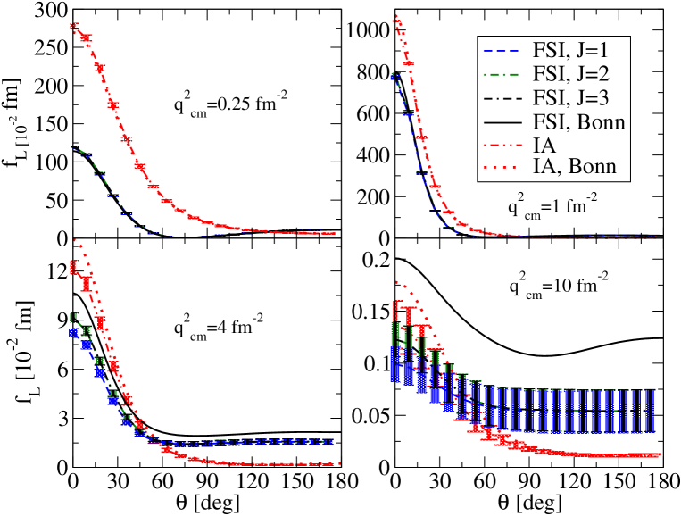
Figure 6: The deuteron electro-disintegration longitudinal response function $f_{L}$ as a function of $\theta$ for $E_{np}=10$ MeV and four different values of $\mathbf{q}_{cm}^{2}$. The error bars are obtained from varying the cutoff $\Lambda=600-1000$ MeV in the LSE. The convergence of the calculation as additional partial waves are included in the computation of the FSI is also shown. Legend as indicated. Here the intrinsic cutoff of SFR TPE is $\widetilde{\Lambda}=800$ MeV.

We first discuss the quasi-free ridge case shown in Fig. 6, i.e., $E_{np}=10$ MeV and $\mathbf{q}_{cm}^{2}=1$ fm^-2. Out of all four panels in Fig. 6, $f_{L}$ receives the least correction from the FSI here, and, as shown in the other three panels, the further away we move from the quasi-free ridge the larger the FSI correction becomes. This can be explained easily by the fact that, at the quasi-free ridge, both nucleons in the deuteron are on the mass shell after being struck by the virtual photon, and no FSI is needed in order to make the final-state particles real. On the other hand, as we move further kinematically from the quasi-free ridge, the FSI must provide a larger energy-momentum transfer to make the proton and neutron become real particles in the final state, and so it becomes more important.

Moreover, for this particular np final-state energy, the quasi-free ridge is the last $\mathbf{q}_{cm}^{2}$ where all the PWIA and FSI results from the two potentials agree. As we increase $\mathbf{q}_{cm}^{2}$ to 4 fm^-2 and above, both our PWIA and FSI results start to diverge away from the corresponding Bonn potential results. The error bars also grow quite significantly for $\mathbf{q}_{cm}^{2}>4$ fm^-2, i.e. $\mathbf{q}_{cm}>400$ MeV, particularly in the FSI. There, where both the deuteron wave functions and the NN t-matrix enter the calculation, the results become highly cutoff-dependent.

We now assess how this uncertainty in the $\chi$EFT $f_{L}$ prediction comes from the uncertainty of the $\chi$EFT deuteron wave function and NN t-matrix. Let’s first look at the quasi-free ridge. From Eq. (33) and Eq. (39), we infer that

$$|\mathbf{p}^{\prime}|\approx\frac{|\mathbf{q}_{cm}|}{2}$$ (40)

at the quasi-free ridge, where the dominant element in the calculation is the deuteron wave function $\Psi_{L}(|\mathbf{p}^{\prime}-\frac{\mathbf{q}_{cm}}{2}\mathbf{|})$. At the quasi-free ridge, the value of the wave-function argument achieves its lowest possible value (for a given $E_{np}$): it is $0$ (for $\theta=0$) increasing to $2|\mathbf{p}^{\prime}|$ (for $\theta=\pi$). Fig. 3 shows that the deuteron wave function $\Psi_{L}(p\mathbf{)}$ given by both the SFR and DR TPE up to NNLO agrees with the one given by the Bonn potential at least up to wave function arguments $\approx 100$ MeV, and dies off quickly at higher momentum. Since the high-momentum component of the wavefunction is almost zero, this suggests that $f_{L}$ calculated from these two potentials should agree with each other at the quasi-free ridge. In fact, as shown in Fig. 7, in quasi-free kinematics the $f_{L}$ given by the SFR TPE up to NNLO does agree with those given by the Bonn potential all the way up to $E_{np}=160$ MeV.

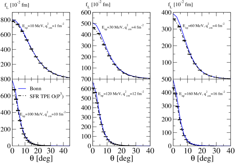
Figure 7: The deuteron electro-disintegration longitudinal response function $f_{L}$ as a function of $\theta$ in various kinematics on or around the “quasi-free ridge”. Here the blue line represents the result given by the Bonn potential with FSI included, and the black double-dash-dotted line denotes the same results given by the SFR TPE up to NNLO. The error bars are obtained from varying the cutoff $\Lambda=600-1000$ MeV in the LSE. The SFR intrinsic cutoff is $\widetilde{\Lambda}=800$ MeV.

To see where the two wave functions start to disagree, we use Fig. 8 as an example ($E_{np}=10$ MeV again, now at more $\mathbf{q}_{cm}^{2}$ values). For $\mathbf{q}_{cm}^{2}\leq 1$ fm^-2, there is no significant difference between results obtained by $\chi$EFT and the Bonn potential. At $\mathbf{q}_{cm}^{2}=4$ fm^-2, the shift due to FSI is roughly the same ($\approx 3.7\times 10^{-2}$ fm at $\theta=0$) for both the NNLO SFR TPE and the Bonn potential. In other words, the FSI has almost the same effect for the two potentials, and the disagreement in the total $f_{L}$ comes (mostly) from the PWIA part. The $\approx 10\%$ difference in the PWIA amplitude originates from the difference between the deuteron wave functions generated by NNLO SFR TPE and the Bonn potentials at around $p=100$ MeV and is not significantly enlarged by the FSI piece where the deuteron wave function is integrated against the NN t-matrix.

Figure 8: The deuteron electro-disintegration longitudinal response function $f_{L}$ as a function of $\theta$ for $E_{np}=10$ MeV, and $\mathbf{q}^{2}_{cm}$ ranging from 0.5 fm^-2 to 16 fm^-2. Here the red dash-double-dotted (dotted) line represents the PWIA results given by the SFR TPE up to NNLO (Bonn), and the black double-dash-dotted (solid) line denotes the FSI results given by the SFR TPE up to NNLO (Bonn). The error bars are obtained from varying the cutoff $\Lambda=600-1000$ MeV in the LSE. The intrinsic cutoff is $\widetilde{\Lambda}=800$ MeV for the SFR TPE up to NNLO.

On the other hand, as we increase $\mathbf{q}_{cm}^{2}$ to $10$ fm^-2 (with $E_{np}=10$ MeV) $f_{L}$ given by the two different potentials starts to have a larger difference in the FSI than in the PWIA—see the lower panels of Fig. 8. Although this final-state energy is well within the range that is fit by our NN potential, one must remember that the deuteron wave function that enters the FSI integral is largest when $|\mathbf{p}|=|\mathbf{q}_{cm}|/2$, and the phase-shift data—where we perform best fit up to $T_{lab}=100$ MeV—only validates our computation of $t(p^{\prime},p;E_{np})$ for $E_{np}\leq 50$ MeV and $p$ up to about $225$ MeV. We infer that it is important for $t(p^{\prime},p;E_{np})$ to at least accurately describe data for the on-shell kinematics corresponding to both $p^{\prime}(\equiv\sqrt{ME_{np}})$ and $p(=|\mathbf{q}_{cm}|\mathbf{/}2)$. If either of these is greater than $225$ MeV, then the difference in the NN t-matrix generated by the SFR TPE up to NNLO and the Bonn potential enters the FSI calculation in addition to any differences in $\Psi_{L}$.

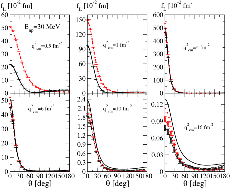
Figure 9: The deuteron electro-disintegration longitudinal response function $f_{L}$ as a function of $\theta$ for $E_{np}=30$ MeV, and $\mathbf{q}^{2}_{cm}$ ranging from 0.5 fm^-2 to 16 fm^-2. Legend as in Fig. 8.

In Fig. 9 we show a similar set of panels to those in Fig. 8, but at $E_{np}=30$ MeV. The agreement between $\chi$EFT and Bonn results is again quite good at low $\mathbf{q}^{2}$, although there is some disagreement at backward angles once FSI is included. This trend in the final result for $f_{L}$ diminishes as we move towards the quasi-free ridge. At the quasi-free ridge the cutoff variation of the $\chi$EFT calculation is small—smaller than for $E_{np}=10$ MeV, because the FSI plays less of a role at this higher energy. The agreement with the Bonn potential is also quite good there. Immediately above the quasi-free ridge these features persist, until $\mathbf{q}^{2}_{cm}\approx 6$ fm^-2, at which point $|\mathbf{q}_{cm}|$ becomes large enough, and the FSI important enough, that agreement cannot be maintained.

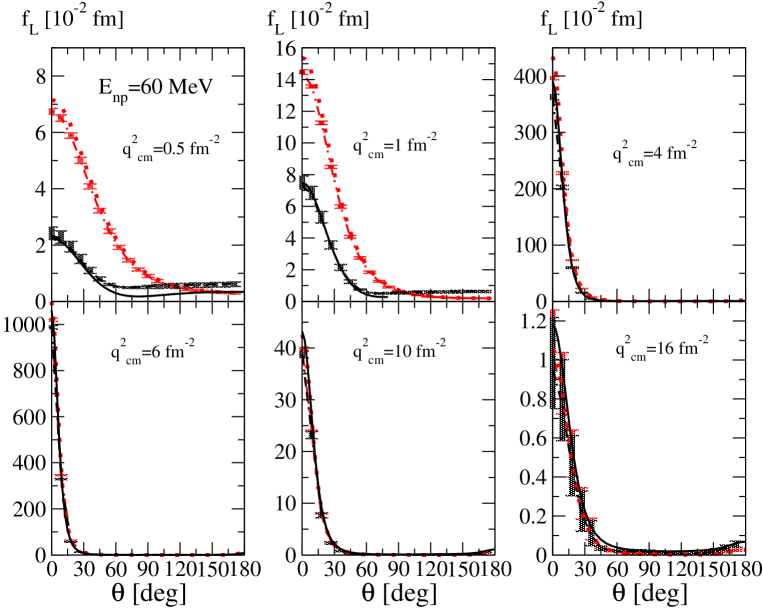
Figure 10: The deuteron electro-disintegration longitudinal response function $f_{L}$ as a function of $\theta$ for $E_{np}=60$ MeV, and $\mathbf{q}^{2}_{cm}$ ranging from 0.5 fm^-2 to 16 fm^-2. Legend as in Fig. 8.

If we now examine $E_{np}=60$ MeV we are already in a regime where the FSI is not trustworthy even if $\mathbf{q}^{2}_{cm}$ is low. This is reflected in the failure of the FSI-included result to encompass the Bonn-potential answer, even within error bars, at $\mathbf{q}^{2}_{cm}=0.5$ fm^-2 (upper-left panel of Fig. 10). But, already by $\mathbf{q}^{2}_{cm}=1$ fm^-2, the Bonn-potential and $\chi$EFT predictions (both with FSI included) are within 10% of each other, with the difference entirely accounted for by the $\chi$EFT result’s variation with the LSE cutoff $\Lambda$. As we move to the quasi-free ridge, and FSI becomes less important, this variation becomes less of a component of the full answer for $f_{L}$. In consequence there is a window, up to $\mathbf{q}^{2}_{cm}\approx 10$ fm^-2, where the cutoff dependence of the final prediction for $f_{L}$ is not sizable. The agreement between $\chi$EFT and the Bonn potential for $f_{L}$ is also good through much of this range. However as $\mathbf{q}^{2}_{cm}$ approaches 10 fm^-2 the Bonn-potential and $\chi$EFT PWIA answers start to differ, especially at small angles. Since the FSI is small in both calculations in this range, that difference is not ameliorated in the full calculation.

We will now summarize the results of the calculations we carried out for $E_{np}=10-160$ MeV and $\mathbf{q}_{cm}^{2}=0.1-25$ fm^-2. The results are generically similar to those displayed above, in that, if we define

$$\mathbf{q}_{qf}^{2}\text{ (fm}^{-2}\text{)}\equiv\frac{E_{np}\text{ (MeV)}}{10}$$ (41)

then our results show that for the kinematic region $E_{np}\leq 60$ MeV and $|\mathbf{q}_{cm}^{2}-\mathbf{q}_{qf}^{2}|$ $<4$ fm^-2, the calculations using $\chi$EFT up to NNLO have $<10$% variation with respect to the cutoff in the LSE . The $\chi$EFT results and those found with the Bonn potential also agree within 10% if $|\mathbf{q}_{cm}^{2}-\mathbf{q}_{qf}^{2}|$ $<2$ fm^-2, for $E_{np}$ at least as high as $160$ MeV. Somewhat remarkably this agreement is possible even in cases where both $E_{np}$ and $\mathbf{q}^{2}_{cm}$ appear to be outside the range of validity of our calculation—as long as we are close to the quasi-free ridge and so details of the FSI remain unimportant.

On the other hand, we emphasize that the $\chi$EFT FSI is reliable for low $|\mathbf{q}_{cm}|$ and low $E_{np}$, see, e.g. first two panels of Fig. 8. Indeed, in the first panel there one might be concerned about the accuracy of our description of the deuteron wave function. The LECs in our chiral potential are obtained through the best fit to the NN phase shifts for $T_{lab}<100$ MeV. In general this does not give the best possible deuteron wavefunction—which is crucial for the PWIA. An alternative would be to perform the renormalization of the LECs in the ${}^{3}S_{1}-^{3}D_{1}$ channel so that some of the deuteron properties, e.g., the binding energy, are very accurately reproduced. We have verified that, by doing this, for $|\mathbf{q}_{cm}^{2}-\mathbf{q}_{qf}^{2}|$ $<4$ fm^-2 the 10% uncertainty due to the variation of the cutoff in the LSE can be reduced to 5%, but only for lower values of $E_{np}(<30$ MeV$)$. Aside from that, it does not improve the discrepancy between the results generated by $\chi$EFT and the Bonn potential. Moreover, for $E_{np}>60$ MeV, the variation of the results with respect to the cutoff becomes larger than before, due to the fact that the NN ${}^{3}S_{1}-^{3}D_{1}$ t-matrix now has worse convergence with respect to the cutoff in the higher energy/momentum region. We conclude that the uncertainty of $f_{L}$ will remain roughly the same unless higher orders in the chiral potential are included.

	$p_{m}$ (MeV)	$|\mathbf{q}_{lab}|$ (MeV)	$E_{np}$ (MeV)	$|\mathbf{q}_{cm}|^{2}$ (fm-2)	$f_{L}/f_{L}^{PWIA}$	$f_{L}^{PWIA}$ (fm)
van der Schaar	39.8	329	42.9	2.66	0.96 $\pm$ 0.03	5.00
et al.	69.9	299	49.5	2.18	0.93 $\pm$ 0.07	1.49
	110	259	59.3	1.62	0.77 $\pm$ 0.14	0.36
	-38.8	419	29.4	4.36	1.08 $\pm$ 0.03	3.15
	39.8	381	53.7	3.51	1.07 $\pm$ 0.03	4.83
	-58.8	503	36.9	6.24	0.96 $\pm$ 0.07	1.00
Ducret et al.	-20	300	17.5	2.26	0.77 $\pm$ 0.02 $\pm$ 0.04	7.91
	-20	400	51.1	2.19	0.88 $\pm$ 0.02 $\pm$ 0.05	1.32
	-20	500	52.2	6.06	0.92 $\pm$ 0.02 $\pm$ 0.05	6.98
	-20	600	75.0	8.53	0.92 $\pm$ 0.02 $\pm$ 0.06	5.44
	-20	670	92.7	10.4	0.87 $\pm$ 0.03 $\pm$ 0.08	4.65
	-100	400	10.3	4.06	0.88 $\pm$ 0.02 $\pm$ 0.06	0.137
	-100	500	22.4	6.26	1.14 $\pm$ 0.02 $\pm$ 0.08	0.135
	-100	600	38.5	8.86	1.15 $\pm$ 0.03 $\pm$ 0.10	0.114
	-100	670	52.0	10.9	1.20 $\pm$ 0.03 $\pm$ 0.12	0.097
	100	200	41.8	0.981	0.51 $\pm$ 0.01 $\pm$ 0.03	0.493
	100	300	64.1	2.16	0.66 $\pm$ 0.01 $\pm$ 0.04	0.492
	100	400	90.1	3.73	0.75 $\pm$ 0.01 $\pm$ 0.04	0.444
	100	500	119	5.66	0.88 $\pm$ 0.02 $\pm$ 0.06	0.385
Jordan et al.	53	402	65	3.9	$f_{L}=$ 1.78 $\pm$ 0.07 $\pm$ 0.15	N/A

Table 1: The first two columns give kinematics quoted in the relevant papers: the missing momentum, and the three-momentum transfer to the nucleus as measured in the lab. frame. The next two columns give the (c.m. frame) quantities we employ for our calculation. The fifth column shows results for $f_{L}/f_{L}^{PWIA}$ were extracted from plots given in Refs. vdS91 ; Du94 ; Jo96 . The first error is the statistical error, while the second is the systematic quoted in the publication. The last column shows $f_{L}^{PWIA}$ evaluated with the Paris potential. The units for the Jordan et al. $f_{L}$ measurement are fm.

	$E_{np}$ (MeV)	$|\mathbf{q}_{cm}|^{2}$ (fm-2)	$f_{L}$ (fm)	$f_{L}^{\chi EFT}$ (fm)
van der Schaar et al.	42.9	2.66	4.59 $\pm$ 0.15	4.06 $\pm$ 0.04
	49.5	2.18	1.31 $\pm$ 0.10	1.09 $\pm$ 0.01
	59.1	1.62	0.265 $\pm$ 0.048	0.218 $\pm$ 0.005
	29.4	4.36	3.46 $\pm$ 0.10	2.78 $\pm$ 0.03
	53.7	3.51	4.84 $\pm$ 0.14	3.92 $\pm$ 0.03
	36.9	6.24	0.998 $\pm$ 0.073	0.911 $\pm$ 0.006
Ducret et al.	17.5	2.26	6.07 $\pm$ 0.24	6.52 $\pm$ 0.06
	51.1	2.19	1.09 $\pm$ 0.04	0.94 $\pm$ 0.01
	52.2	6.06	6.63 $\pm$ 0.22	6.36 $\pm$ 0.06
	75.0	8.53	5.50 $\pm$ 0.18	5.23 $\pm$ 0.05
	92.7	10.4	4.61 $\pm$ 0.16	5.02 $\pm$ 0.81
	10.2	4.06	0.119 $\pm$ 0.004	0.096 $\pm$ 0.003
	22.4	6.26	0.155 $\pm$ 0.005	0.116 $\pm$ 0.002
	38.5	8.86	0.136 $\pm$ 0.005	0.105 $\pm$ 0.001
	52.0	10.9	0.124 $\pm$ 0.004	0.091 $\pm$ 0.001
	41.7	0.981	0.245 $\pm$ 0.010	0.271 $\pm$ 0.005
	64.1	2.16	0.306 $\pm$ 0.015	0.326 $\pm$ 0.006
	90.1	3.73	0.298 $\pm$ 0.012	0.310 $\pm$ 0.004
	119	5.66	0.280 $\pm$ 0.013	0.261 $\pm$ 0.002
Jordan et al.	65.2	3.9	1.78 $\pm$ 0.07	2.15 $\pm$ 0.02

Table 2: The experimental number quoted in the second-last column is the result of multiplying the final two rows of the previous table (with the exception of the Jordan et al. point). Only statistical errors are listed for the experimental result presented in this table, since systematic errors are accounted for separately. $f_{L}^{\chi EFT}$ is an average of $\chi$EFT calculations that include both PWIA and FSI pieces and use cutoffs ranging from 600–1000 MeV, with the error bar indicating the size of the spread.

Finally, we compare our results with data for the longitudinal structure function published in Refs. vdS91 ; Du94 ; Jo96 . The kinematics and data for $f_{L}$ are listed in Table 1. The experiments of van der Schaar et al. vdS91 and Ducret et al. Du94 give their data as ratios between the measured longitudinal response and that predicted by a Paris-potential La80 impulse-approximation calculation. For those two experiments we have calculated $f_{L}^{PWIA}$ at the pertinent momentum using the Paris-potential deuteron wave-function parameterization of Ref. La81 . The result for $f_{L}$ given in Table 2 is then obtained by multiplying the final two columns in Table 1 together (with the obvious exception of the single data point of Jordan et al. Jo96 , where the publication gives $f_{L}$ directly). Table 2 compares these experimental results for $f_{L}$ with those from our $\chi$EFT calculations using the SFR NNLO potential and cutoffs of 0.6 to 1 GeV.

In fact, we find significant sensitivity of both the Paris IA and the $\chi$EFT result to the value of $E_{np}$ chosen. The value of $E_{np}$ listed here is obtained from the initial-state kinematics given in the publications, using the relativistic energy-momentum relation. Using the value of $E_{np}$ found from the final-state kinematics to compute $f_{L}^{PWIA}$ produces results that differ by more than the quoted uncertainties on $f_{L}/f_{L}^{PWIA}$. This makes us think that further details of the experiments, e.g., acceptances, are needed in order to provide a completely meaningful comparison between theory and data.

Nevertheless, some trends are already clear from the straightforward comparison between theory and data that can be made without detailed knowledge of the experiments. For the $p_{m}=-20$ MeV data (Ducret et al.) the $\chi$EFT calculations are in good agreement with the data, once the experiment’s $\approx 6$% systematic is accounted for. For example, multiplying the Ducret et al. data by 1.015, we find that the $\chi$EFT prediction is within 1.3 (combined theory and statistical uncertainty of the measurement) $\sigma$ for all but the $E_{np}=51.1$ MeV data point. The agreement for $p_{m}=100$ MeV is also very good—even at the highest $\mathbf{q}_{cm}^{2}$ of almost 6 fm^-2. For the rest of the Ducret et al. data set, taken at $p_{m}=-100$ MeV, the $\chi$EFT calculation is systematically below the data, and this cannot be attributed to normalization uncertainty—at least not within the quoted systematic.

Similarly, the van der Schaar et al. data are (with one exception) all underpredicted by $\chi$EFT at this order. This problem persists even if the entire 7% systematic uncertainty quoted in Ref. vdS91 is assigned to the experimental normalization. The disagreement worsens as $\mathbf{q}_{cm}^{2}$ increases, with the only experimental point for $\mathbf{q}_{cm}^{2}<2$ fm^-2 agreeing with the $\chi$EFT prediction while points in the range $2~{}\mathrm{fm}^{-2}<\mathbf{q}_{cm}^{2}<3~{}\mathrm{fm}^{-2}$ have $\chi$EFT 1-3$\sigma$ below the data (depending on how the experimental normalization is treated). The disagreement between $\chi$EFT and data becomes dramatic at higher $\mathbf{q}_{cm}^{2}$.

Similar under-prediction also occurs when Arenhövel’s Bonn-potential calculation is compared to these data, so the difficulty appears generic to calculations employing only the one-body operator for $J_{0}$. It will be interesting to explore whether higher-order corrections to the NN charge operator in $\chi$EFT can redress the difference seen here between theory and experiment. It is also worth noting that the uncertainty due to cutoff variation in the $\chi$EFT result is very small for most cases. This leads us to question whether varying the cutoff between 600 MeV and 1 GeV adequately estimates the uncertainty in the $\chi$EFT result due to higher-order effects.

VI Conclusion

We have computed the longitudinal structure function of the deuteron, $f_{L}$, in $\chi$EFT, including effects up to $\mathcal{O}(P^{3})$ relative to leading order in the standard counting. Comparison with calculations of Arenhövel et al., which use the Bonn potential, indicates good agreement at low energies ($E_{np}\leq 60$ MeV) and for $\mathbf{q}^{2}$ which are not very distant ($<4$ fm^-2) from the quasi-free ridge. We also use the $\Lambda$ dependence of the $\chi$EFT calculation as a diagnostic, to find kinematic regions where the final result for $f_{L}$ is sensitive to short-distance components in the evaluation of the final-state interaction. If significant $\Lambda$ dependence is present it suggests sensitivity to such effects, which may mean that both the $\chi$EFT calculation and the Bonn-potential calculation do not capture the full dynamics present in $f_{L}$. With this caveat in mind, we find that our calculations are able to describe data from Saclay, NIKHEF, and Bates, on the longitudinal structure function, either within a more restricted kinematic region (compared to the region where our results agree with Bonn potential), or by allowing somewhat expanded combined (statistical + systematic + theory) error bars. We also notice that both $\chi$EFT and Bonn potential give a similar trend of under-prediction of the experimental $f_{L}$ with increasing $\mathbf{q}_{cm}^{2}$. Further studies are needed to understand the origin of this discrepancy.

In fact, the $\chi$EFT calculation is in good agreement with the Bonn potential and with the data to surprisingly high energies and $\mathbf{q}^{2}$ as long as one stays on (or near) the quasi-free ridge. This suggests that a different counting may be needed for this reaction, one where the expansion is not in the naive kinematic variables, $|\mathbf{p}^{\prime}|$ and $|\mathbf{q}|$, but instead, perhaps where some account is taken of the dominance of the PWIA part of the matrix element for sufficiently high energies ($E_{np}>30$ MeV) and sufficiently low values of the “missing momentum” $|\mathbf{p}-\frac{\mathbf{q}}{2}|$.

In the future, the recent $\chi$EFT calculations of elastic scattering on tri-nucleons Pa12 could be extended to electrodisintegration, and compared with data on that reaction exp_dis_3n . However, a more obvious and immediately necessary next step is to extend this $\chi$EFT calculation to other structure functions. The three-current operator $\mathbf{J}$ has also been computed to three orders relative to leading order Ko09 ; Ko11 ; Pa09 ; Pa11 , and comparison of $f_{T}$, $f_{LT}$, and $f_{TT}$ with data (and Bonn-potential calculations) would be an important test of the domain of validity of the $\chi$EFT expansion for that object.

In closing, we reiterate that such a test can be rendered unambiguous because the results presented here show the regions in which the $\chi$EFT expansion for the PWIA and FSI pieces of the deuteron electrodisintegration process are under control. The absence of any NN mechanisms in the charge operator up to the order considered makes the $f_{L}$ presented here a prediction once the NN potential is fixed by the fit to NN data. The fact that we find good agreement with both $f_{L}$ data and other theories in a broad kinematic range provides further reassurance (see also Refs. Ph07 ; Ko12 ) that $\chi$EFT does a good job of describing deuteron structure for internal relative momenta $<0.2$ GeV.

- (1) S. Weinberg, Phys. Lett. B 251, 288 (1990); Nucl. Phys. B 363, 3 (1991).
- (2) E. Epelbaum, H. -W. Hammer and U. -G. Meißner, Rev. Mod. Phys. 81, 1773 (2009).
- (3) E. Epelbaum and U. -G. Meißner, Ann. Rev. Nucl. Part. Sci. 62 159-185 (2012).
- (4) S. Kölling, E. Epelbaum, H. Krebs and U.-G. Meißner, Phys. Rev. C 80, 045502 (2009).
- (5) S. Kölling, E. Epelbaum, H. Krebs and U.-G. Meißner, Phys. Rev. C 84, 054008 (2011).
- (6) S. Pastore, R. Schiavilla and J. L. Goity, Phys. Rev. C 78, 064002 (2008).
- (7) S. Pastore, L. Girlanda, R. Schiavilla, M. Viviani and R. B. Wiringa, Phys. Rev. C 80, 034004 (2009).
- (8) S. Pastore, L. Girlanda, R. Schiavilla and M. Viviani, Phys. Rev. C 84, 024001 (2011).
- (9) M. Piarulli, L. Girlanda, L. E. Marcucci, S. Pastore, R. Schiavilla and M. Viviani, Phys. Rev. C 87, 014006 (2013).
- (10) D. R. Phillips, J. Phys. G 34, 365-388, (2007).
- (11) D. R. Phillips, Phys. Lett. B 567, 12 (2003).
- (12) D. R. Phillips and T. D. Cohen, Nucl. Phys. A 668, 45 (2000).
- (13) M. Walzl and U. G. Meißner, Phys. Lett. B 513, 37 (2001).
- (14) S. Kölling, E. Epelbaum and D. R. Phillips, Phys. Rev. C 86, 047001 (2012).
- (15) L. Girlanda, A. Kievsky, L. E. Marcucci, S. Pastore, R. Schiavilla and M. Viviani, Phys. Rev. Lett. 105, 232502 (2010).
- (16) S. Pastore, S. C. Pieper, R. Schiavilla and R. B. Wiringa, Phys. Rev. C 87, 035503 (2013).
- (17) H. Arenhövel, W. Leidemann and E. Tomusiak, Phys. Rev. C 46, 455 (1992).
- (18) H. Arenhövel et al, Z. Phys. A 331, 123-138 (1988).
- (19) H. Arenhövel, W. Leidemann and E. Tomusiak, Phys. Rev. C 43, 1022 (1991).
- (20) H. Arenhövel, W. Leidemann and E. L. Tomusiak, Few Body Syst. 28, 147 (2000).
- (21) H. Arenhövel, W. Leidemann and E. L. Tomusiak, Eur. Phys. J. A 14, 491 (2002).
- (22) H. Arenhövel, W. Leidemann and E. L. Tomusiak, Eur. Phys. J. A 23, 147 (2005).
- (23) C.-J. Yang, Ch. Elster and D. R. Phillips Phys. Rev. C 77, 014002 (2008).
- (24) D. Eiras and J. Soto, Eur. Phys. J. A 17, 89 (2003).
- (25) A. Nogga, R.G.E. Timmermans and U. van Kolck, Phys. Rev. C 72, 054006 (2005).
- (26) M. C. Birse, Phys. Rev. C 74, 014003 (2006).
- (27) M. Pavon Valderrama and E. Ruiz Arriola, Phys. Rev. C 74, 064004 (2006) [Erratum-ibid. C 75, 059905 (2007)].
- (28) C.-J. Yang, Ch. Elster and D. R. Phillips, Phys. Rev. C 80, 034002 (2009).
- (29) C.-J. Yang, Ch. Elster and D. R. Phillips, Phys. Rev. C 80, 044002 (2009).
- (30) E. P. Wigner, Phys. Rev. 98, 145 (1955).
- (31) D. R. Phillips and T. D. Cohen, Phys. Lett. B 390, 7 (1997).
- (32) K. A. Scaldeferri, D. R. Phillips, C. W. Kao and T. D. Cohen, Phys. Rev. C 56, 679 (1997).
- (33) C. Ordonez, L. Ray and U. van Kolck, Phys. Rev. C 53, 2086 (1996).
- (34) D. R. Entem and R. Machleidt Phys. Lett. B 524, 93 2002.
- (35) E. Epelbaum, W. Glöckle, and U.-G. Meißner, Nucl. Phys. A 671, 295 (2000).
- (36) D. R. Entem and R. Machleidt, Phys. Rev. C 68, 041001(R) (2003).
- (37) E. Epelbaum, W. Glöckle and U-G. Meißner, Nucl. Phys. A 747, 362 (2005).
- (38) G. P. Lepage, arXiv:nucl-th/9706029.
- (39) E. Epelbaum and Ulf-G. Meißner, arXiv:nucl-th/0609037.
- (40) M. C. Birse, PoS CD 09, 078 (2009) [arXiv:0909.4641 [nucl-th]].
- (41) D. R. Phillips, PoS CD 12, 013 (2012) [arXiv:1302.5959 [nucl-th]].
- (42) M. van der Schaar, H. Arenhovel, T. S. Bauer, H. P. Blok, H. J. Bulten, M. Daman, R. Ent and E. Hummel et al., Phys. Rev. Lett. 66, 2855 (1991).
- (43) J. E. Ducret, M. Bernheim, J. F. Danel, L. Lakehal-Ayat, J. M. Le Goff, A. Magnon, C. Marchand and J. Morgenstern et al., Phys. Rev. C 49, 1783 (1994).
- (44) D. Jordan, T. McIlvain, R. Alarcon, R. Beck, W. Bertozzi, V. Bhushan, W. Boeglin and J. P. Chen et al., Phys. Rev. Lett. 76, 1579 (1996).
- (45) M. Bernheim et al., Nucl. Phys. A 365, 349 (1981).
- (46) S. Turck-Chieze, P. Barreau, M. Bernheim, P. Bradu, Z. E. Meziani, J. Morgenstern, A. Bussiere and G. P. Capitani et al., Phys. Lett. B 142, 145 (1984).
- (47) H. Breuker, V. Burkert, E. Ehses, U. Hartfiel, G. Knop, G. Krosen, J. Langen and M. Leenen et al., Nucl. Phys. A 455, 641 (1986).
- (48) K. I. Blomqvist, W. U. Boeglin, R. Bohm, M. Distler, R. Edelhoff, I. Ewald, R. Florizone and J. Friedrich et al., Phys. Lett. B 424, 33 (1998).
- (49) N. Ryezayeva et al., Phys. Rev. Lett. 100, 172501 (2008).
- (50) M. van der Schaar, H. Arenhovel, H. P. Blok, H. J. Bulten, E. Hummel, E. Jans, L. Lapikas and G. van der Steenhoven et al., Phys. Rev. Lett. 68, 776 (1992).
- (51) T. Tamae, H. Kawahara, A. Tanaka, M. Nomura, K. Namai, M. Sugawara, Y. Kawazoe and H. Tsubota et al., Phys. Rev. Lett. 59, 2919 (1987).
- (52) F. Frommberger, D. Durek, R. Gothe, G. Happe, C. Hueffer, D. Jakob, M. Jaschke and G. Knop et al., Phys. Lett. B 339, 17 (1994).
- (53) W.-J. Kasdorp et al., Phys. Lett. B 393, 42 (1997).
- (54) Z. L. Zhou et al. [MIT-Bates OOPS Collaboration], Phys. Rev. Lett. 87, 172301 (2001).
- (55) W. U. Boeglin, H. Arenhovel, K. I. Blomqvist, R. Bohm, M. Distler, R. Edelhoff, I. Ewald and R. Florizone et al., Phys. Rev. C 78, 054001 (2008).
- (56) P. E. Ulmer, K. A. Aniol, H. Arenhovel, J. P. Chen, E. Chudakov, D. Crovelli, J. M. Finn and K. G. Fissum et al., Phys. Rev. Lett. 89, 062301 (2002).
- (57) W. U. Boeglin et al. [Hall A Collaboration], Phys. Rev. Lett. 107, 262501 (2011).
- (58) S. Jeschonnek and J. W. Van Orden, Phys. Rev. C 78, 014007 (2008).
- (59) S. Jeschonnek and J. W. Van Orden, Phys. Rev. C 81, 014008 (2010).
- (60) D. Rozpedzik, J. Golak, S. Kölling, E. Epelbaum, R. Skibinski, H. Witala and H. Krebs, Phys. Rev. C 83, 064004 (2011).
- (61) S. Christlmeier and H. W. Grießhammer, Phys. Rev. C 77, 064001 (2008).
- (62) P. von Neumann-Cosel et al., Phys. Rev. Lett. 88, 202304 (2002).
- (63) V. Bernard, N. Kaiser, J. Kambor and U. G. Meißner, Nucl. Phys. B 388, 315 (1992).
- (64) D. R. Phillips, J. Phys. G 36, 104004 (2009).
- (65) See http://nn-online.org/
- (66) V. G. J. Stoks, R. A. M. Klomp, M. C. M. Rentmeester and J. J. de Swart, Phys. Rev. C 48, 792 (1993).
- (67) M. A. Belushkin, H.-W. Hammer and Ulf-G. Meißner, Phys. Rev. C 75, 035202 (2007).
- (68) H. Arenhövel, private communication.
- (69) R. Machleidt, K. Holinde and C. Elster, Phys. Rept. 149, 1 (1987).
- (70) M. Lacombe, B. Loiseau, J. M. Richard, R. Vinh Mau, J. Cote, P. Pires and R. De Tourreil, Phys. Rev. C 21, 861 (1980).
- (71) M. Lacombe, B. Loiseau, R. Vinh Mau, J. Cote, P. Pires and R. de Tourreil, Phys. Lett. B 101, 139 (1981).
- (72) P.H.M. Keizer, et al., Phys. Lett. B 157 255 (1985); P.H.M. Keizer, et al., Phys. Lett. B 197 29 (1987); P.H.M. Keizer, Ph.D. Thesis, Amsterdam 1986.