A methodology for detecting and exploring non-convulsive seizures in patients with SAH

Abstract

A methodology for understanding and detecting nonconvulsive seizures in individuals with subarachnoid hemorrhage is introduced. Specifically, beginning with an EEG signal, the power spectrum is estimated yielding a multivariate time series which is then analyzed using empirical orthogonal functional analysis. This methodology allows for easy identification and observation of seizures that are otherwise only identifiable though expert analysis of the raw EEG.

1 Introduction

Seizure detection in EEG data has a long history [santa_fe_time_series_prediction, larry_neuroscience_book, partha_brain_book]. In fact, seizure detection is developed to the point where medical instrument companies have proprietary seizure detection algorithms. Nevertheless, automated seizure detection is not particularly effective. Moreover, most seizure detection is carried out in the context of epilepsy. Here we develop a new methodology for understanding and detecting seizure in a different context, in patients with a aneurysmal subarachnoid hemorrhage (SAH). The context is important because SAH is a serious clinical condition that affects a broad population. And the context is different from the more standard epilepsy context; seizures in individuals with SAH are not well understood, may be diverse in type, and may affect recovery in different ways. Because of the potential diversity in seizure in SAH patients, we aim to both detect seizure events and understand and phenotype the different seizure types. Our methodology is based applying several targeted levels of analysis to the original EEG signal; here this methodology entails estimating a power spectrum from EEG data and then applying empirical orthogonal functional analysis (EOF)to the power spectrum (PS).

2 Seizures in individuals with SAH

Aneurysmal subarachnoid hemorrhage (SAH) occurs when blood enters the subarachnoid space, located between the arachnoid membrane and the pia mater surrounding the brain, from a ruptured dilated cerebral blood vessel. SAH affects up to 30,000 Americans annually carrying a huge public health burden. Secondary complications such as nonconvulsive seizures (NCSz) contribute significantly to poor outcome. These seizures are different from convulsive seizures as the patients have no or minimal symptoms other than decreased mental status while the brain is seizing. There is a great deal of evidence that suggests that additional brain injury occurs secondary to NCSz [subarachnoid_seizures_I].

Treatment is available but diagnosis poses major challenges as automated detection algorithms to date have very poor accuracy. Controversy exists regarding the preferred treatment regimen but unanimously experts agree that the time to initiate treatment is much more important than the choice of seizure medication. Detection algorithms fall short as surface EEG is notoriously contaminated by artifact. Some sources of artifacts include poor contact between EEG electrodes and scalp, sweat artifact, electrical artifact, and many more. Intracrotical depth electrodes are increasingly placed together with other invasive brain monitoring devices and have the huge advantage of a better signal to noise ratio. Signals from such sources would be an ideal to further develop seizure detection algorithms with better specificity and sensitivity for seizures.

Diversity among seizures

Seizures after acute brain injury show a great deal of phenotypical variability. For example, approximately half of the seizures remain focal and do not spread to other brain regions. Patterns of seizures further differ greatly in terms of maximum frequency, amplitude, duration, and background in between discharges. The pathophysiological significance of these differences is unknown but to study these differences accurate characterization of patterns is the first step.

3 Seizure detection and analysis

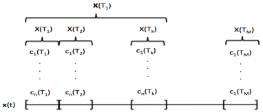
Figure 1: Broad view of our seizure analysis methodology. Given a time series ($\mathbf{x}(t)$), we estimate a power spectra at fixed intervals yielding powers per frequency ($c_{i}(T_{j})$) that are then treated as a multi-variate time series ($\mathbf{X}(T_{i})$) that is then studied using EOF analysis.

General decomposition of a time series

Begin with a time series of length $MT$, $\mathbf{x}(MT)=(x(1),x(2),\cdots,x(MT))$. Assume over the time period or window of calculation that the time series is ergodic and obeys the weak stationarity property [koopmans, statistical_analysis_climate_book]. We will, for now, split the time series $\mathbf{x}(MT)$ into $M$ components, indexed by $k$ and denoted by $\mathbf{x}_{k}(t)$. The time series can be decomposed into $n$ orthogonal components, or

$$\mathbf{x}_{k}(t)=\sum_{i=j}^{N}c_{j}\mathbf{e}_{j}$$ (1)

$\mathbf{e}_{j}$ is an orthogonal basis functions and $c_{j}$ is the amplitude of that given basis function. In this paper, we will begin with a time series of finite length, $MT$, split it into $M$ components of length $T$, and then decompose the disjoint time series in two different steps to achieve a useful representation of seizure dynamics.

Power spectra decomposition of EEG data

It is well known [koopmans] that a way to represent a time series is via a decomposition into a set of $2n$ frequencies, $\lambda_{j}$, or

$$\mathbf{x}_{k}(t)=\sum_{j=-n}^{n}c_{j}e^{i\lambda_{j}t};$$ (2)

this representation of $\mathbf{x}_{k}(t)$ is called the Fourier transform [whezyg, koopmans, fourierO_dirichlet] of $\mathbf{x}_{k}(t)$. In this framework $\mathbf{x}_{k}(t)$ is conceptualized as a collection of harmonic terms parameterized by frequency. Each frequency has an instantaneous power associated with it $|c_{j}|^{2}$; or $|c_{j}|^{2}$ is the power of $x(t)$ at frequency $\lambda_{j}$. Intuitively the power at a frequency quantifies how much of $\mathbf{x}(t)$’s signal is represented by the orthogonal component, or harmonic term, $c_{j}e^{i\lambda_{j}t}$, over the time window of length $T$. The power calculation yields the vector of powers for given frequencies, $X_{k}(t)=(|c_{1}|^{2},|c_{2}|^{2},\cdots,|c_{n}|^{2})$, for each of the $M$ time series. Finally, by Parseval’s theorem [whezyg, koopmans] the total power in frequency space is equal to the variance in state space, or:

$$\sigma(\mathbf{x}_{k}(T))=P(\mathbf{x}_{k}(T)) =\frac{1}{T}\sum_{t=1}^{T}x^{2}(t)$$ (3)

$$=\sum_{j=-n}^{n}|c_{j}|^{2}$$ (4)

Empirical orthogonal functional analysis

To study the time series of the vector of power per frequency, $\mathbf{X}(T_{k})$, a multivariate time series, we must generalize to multivariate, or matrix decompositions. For the moment we will ignore the meaning of the time points (powers) and abstract the $|c_{j}|^{2}$’s to be any variable dependent on time.

Consider a matrix of time series, where the columns index the time points, and the rows index the variables (e.g., the frequencies). Assume we have de-trended $\mathbf{X}(T_{k})$ such that it is mean zero. Associated with $\mathbf{X}(T_{k})$ is its covariance matrix, $\Sigma(T_{k})$. By construction $\Sigma$ is Hermitian so the eigenvalues are non-negative and there will always exist an orthogonal basis (i.e., the eigenvectors are orthogonal). We can decompose $\mathbf{X}(T_{k})$ by the orthogonal directions of maximum variance which is equivalent to (cf. section 13.1 in [statistical_analysis_climate_book]) decomposing $\mathbf{X}(T_{k})$ into eigenvectors (e.g., the generalized $\mathbf{e}_{j}$’s from Eq. 1) corresponding to the eigenvectors of $\Sigma(T_{k})$ in descending order. In this way, the first EOF is the pattern representing the maximum variance within $\mathbf{X}(T_{k})$; written more mathematically, the first EOF is the eigenvector that minimizes $E(||\mathbf{X}-\langle\mathbf{X},\mathbf{e}\rangle\mathbf{e}||^{2})$. Note that $\mathbf{X}(T_{k})$ must be at least a full rank matrix which in practice means that $k\geq n$.

We visualize the EOFs individually as vectors, usually restricted to the first EOF, creating a multivariate time series of length $M$. Moreover, to we also estimate and plot the time-dependent fraction of energy or variance represented by the EOF being plotted. Recall that the total power (variance), is the sum of the eigenvalues (the trace) of $\Sigma(T_{k})$, or $\sigma(\mathbf{X}(T_{k}))=\sum_{j=1}^{n}\lambda_{j}$. Using this, the fraction of the variance that EOF $j$ represents is $\frac{\lambda_{j}}{\sigma(\mathbf{X}(T_{k})}$.

Explicit details of the PS and EOF computations

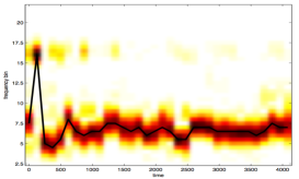
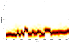
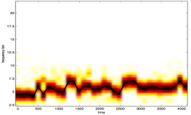
Figure 4: EOF of the PS of the EEG for the left, right, and whole brain (left to right) respectively; note depth seizure event is only apparent in the EOF of the left side of the brain and is indicated by a qualitative change in the EOF signal as realized via a larger number and different set of frequencies contributing to the variance of the signal.

The explicit algorithm we used in this paper follows four steps: (i) collect a time series of PS data, which is estimated by the machinery used to collect EEG data; (ii) determine a suitable EOF window size, noting that $k\geq n$, thus creating the $\mathbf{X}(T_{j})$’s; (iii) estimate the EOF on non-overlapping time windows of the PS data, the $\mathbf{X}(T_{j})$’s; and (iv) plot the first EOF, a $n$-dimensional vector, in time (cf. Figs. 2 and 4).

Interpretation of the EOFs of the time series of PS of a time series

Moving back into the context where $\mathbf{X}(T_{k})$ is a matrix of time series of power per frequency, the interpretation of PS, the first EOF, and the first EOF of the PS are as follows.

Power spectrum of the time series: a time series can be decomposed and represented as energy or power (if integrated over time) of the frequencies that compose the time series. Or, written differently, the time series can be rewritten in terms of power (variance) per orthogonal basis element. In this situation, the basis elements are not chosen to maximize any quantity, but rather as the frequencies present in the data.

First EOF of a multivariate time series: the orthogonal direction that represents the direction of greatest (or maximized) energy or variance and can include portions of different frequencies (e.g., $3$ Hz accounts for $20\%$ , $5$ Hz accounts for $40\%$, etc.); the first EOF is a vector that specifies what proportions of which frequencies make up the orthogonal vector in the direction of the maximum energy or variance.

First EOF of the PS of a time series: the ranked (or ordered) proportional selection of frequencies that contribute the most energy without overlapping (i.e., along the orthogonal component that captures or represents the maximum amount of energy). This is equivalent to identifying the frequencies, by proportion, that contribute the most to variance, or energy in the EEG signal. Because variance and energy are synonymous, the first EOF of the PS of a time series reveals the frequencies within the EGG signal that are the most active, important, present, or energetic.

4 Results

Identifying high resolution EOF features before and after manually identified seizure events.

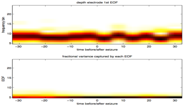
Figure 2: First EOF (top) and relative importance (fractional variance) of each EOF versus time before and after seizure for power spectra of an EEG time series. Blue implies no contribution, red implies maximum contribution to the EOF.

To study the nature of depth seizures in SAH patients, we applied EOF analysis to the PS of the EEG for $n=20$ ranging from $1$ to $20$ Hz recorded at $5$ second intervals ($T=5min$, $k=60$) $30$ minutes before and after seizure ($M=60min$) for several single patient with a SAH; because $k=60$ and $n=20$, without pathologies $\mathbf{X}(T_{k})$ will be full rank. The seizure onsets were manually identified by a neurointensivist. The signal via EOF of the PS of the EEG revealed is striking: at the onset of seizure, the period of oscillation between the high-variance frequencies changes; in the specific patient shown in Fig. 2 from the oscillation in frequency changes period from $25$ to $12$ minutes. Moreover, as the seizure onsets, the amount of variance represented by the first EOF increases dramatically, as can be seen in Fig. 2. This implies that as the during the seizure, the set of excited frequencies is severely constrained. It is hoped that temporal signatures such as these can be generalized to better understand seizure, and to phenotype different types of seizure in SAH patients.

Seizure visualization and detection prior to manual seizure identification.

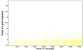
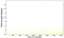
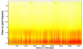
Figure 3: PS of the EEG for the left, right, and whole brain (left to right) respectively. Note, the left and right portions figures are not empty, but rather the range the variables take is very large and thus difficult to visualize. Finally, note that no seizure-like event is evident.

A subset of the SAH patients we study have a depth electrode inserted in their brain to monitor electrical activity for clinical reasons. A subset, $18$ of $48$, of these patients displayed a “depth seizure,” or a seizure that was not easily identifiable from the surface EEG. In our example, the depth seizure was manually identified from the raw EEG collected from the depth probe. Here the PS of the EEG was recorded once a minute with an $n=40$ spit into half a Hz intervals ranging from 1-20 Hz for the entire length of the patient stay. Here we set $T=40$ minutes, making $n=k=40$, allowing again for $\mathbf{X}(T_{k})$ to be of full rank. Because of the lower resolution of the recordings we ignore fine scale features and work to detect seizure by identifying abrupt changes in the active frequencies. Figure 3 shows the PS of the surface EEG for the left, right, and whole brain respectively. In these plots, no discernible seizure-like structure is evident. The EOF of the PS signals tell another story. In this patient the feature we would hope to see, abrupt changes in the frequencies with energy, are clearly visable in the left brain only; neither the whole brain nor the right brain have a single strong enough to identify a seizure-like event in the EOF signal. This corroborates what we expect in half of the depth seizure cases — a localized seizure event that is not propagating through the rest of the brain. Therefore, in this example, applying the EOF to the PS of the surface EEG can help identify depth seizure events using surface EEG data that are only identifiable manually using the depth EEG and are manually unidentifiable using the PS of either the depth or the surface EEG alone.

Seizure identification in a small population of SAH patients with and without seizure.

A first step toward using an EOF signal to define a seizure phenotype is to determine whether an EOF signal can be used to identify seizure by humans at a broad level. Using a data set consisting of $26$ patients, $1$ with a surface and $12$ with depth seizures, we compared EOF visualization to PS visualization in correctly identifying seizures according to a gold standard generated by a trained neuroscientist. Accuracy was $88\%$ for EOF versus $48\%$ for PS, and the difference was statistically significantly different by McNemar’s test ($p=0.008$) [mcnemars_test]. Similarly, using the EOF of the PS there is a strong, statistically significant linear correlation ($\rho=0.76$, $p=10^{-5}$) between EOF-identified seizure and the gold standard. There was no linear correlation between the PS identified seizure and the gold standard. Relative to the data set here, the EOF was not useful for differentiating depth versus surface seizure; this lack of effectiveness is likely due to sample size (correlation for depth identification was strong but not statistically significant).

5 Discussion

EOF analysis of the PS of EEG highlights the characteristics of EEG that define seizure in SAH patients. Moreover, the EOF of the PS of the EEG makes manual identification of seizure significantly easier and more reliable. As is often the case, multiple levels of data analysis, e.g., estimating the EOF of the PS of the EEG, can be very useful for revealing the important temporal content.

Given the likelihood that seizures in SAH patients have different implications for different populations of patients (e.g., older patients, patients with great injury, etc.), discovering and quantifying the differentiating temporal signatures and tying them to outcomes will be of critical significance for both understanding and treating seizure in patients with SAH. Nevertheless scientifically controlled collection of EEG data for SAH patients are rare if nonexistent. Here we show that it is possible to use physiologic data collected for clinical reasons to better understand SAH-based pathophysiology, even though the data are collected outside of a scientifically controlled environment and contain noise, missing values, clinical intervention effects, and nonstationary trends. Nevertheless, much work remains both to automate seizure detection in SAH patients using the EOF of the PS, and to statistically define the temporal signatures that can be used to differentiate patient health and predict patient outcome.