Chern Simons duality with a fundamental boson and fermion

Sachin Jain1, Shiraz Minwalla2, Shuichi Yokoyama3
Department of Theoretical Physics, Tata Institute of Fundamental Research,
Homi Bhabha Road, Mumbai 400005, India
E-mail: 1sachin, 2minwalla, 3yokoyama(at)theory.tifr.res.in
Abstract:

We compute the thermal free energy for all renormalizable Chern Simon theories coupled to a single fundamental bosonic and fermionic field in the ’t Hooft large $N$ limit. We use our results to conjecture a strong weak coupling duality invariance for this class of theories. Our conjectured duality reduces to Giveon Kutasov duality when restricted to ${\cal N}=2$ supersymmetric theories and to an earlier conjectured bosonization duality in an appropriate decoupling limit. Consequently the bosonization duality may be regarded as a deformation of Giveon Kutasov duality, suggesting that it is true even at large but finite $N$.

preprint: TIFR/TH/13-17

1 Introduction

Three dimensional Chern Simons $U(N)$ gauge theories coupled to matter fields are interesting from several points of view. These theories have applications as diverse as quantum hall physics [1, 2], the topology of three manifolds [3] and the study of quantum gravity via the AdS/CFT correspondence [4].

It has recently been realized that vector Chern Simons theories (i.e. Chern Simons theories whose matter fields are all in the fundamental of $U(N)$) are ‘solvable’ in the large $N$ limit. We now have explicit formulae for the spectrum of single sum operators, three point correlation functions and thermal partition functions for some of these theories [5, 6, 7, 8, 9, 10, 11, 12, 13, 14, 15, 16]. These exact results have already led to the discovery of new non supersymmetric level rank dualities between classes of such theories. The existence of such a duality was first speculated on in [5]; concrete evidence for such a duality was provided by the study of three point functions in [7, 8]. The transformation of parameters under duality was first worked out in [9] (based on correlation function computations, see also [14]); this paper also made the first definite conjecture for such a duality. The equality of free energies of dual pairs was established in [13, 15, 16].

Vector matter Chern Simons theories have also been conjectured to admit dual bulk descriptions as a theory of higher spin fields [5, 6, 17]. It thus appears that these theories are dynamically rich even in the analytically tractable large $N$ limit.

In this note we study the most general renormalizable $U(N)$ Chern Simons theory coupled to a single fundamental scalar and fermion field in the large $N$ limit. In particular we use the methods of [5, 10, 13, 15, 11] to exactly determine the quantum corrected pole masses of the propagating bosonic and fermionic fields in this theory. We also determine the exact thermal partition function of these theories as a function of temperature, chemical potentials and couplings. We use our results to propose a level rank type strong weak coupling duality map that relates pairs of these theories, generalizing an earlier proposal by [13].

A special case of the theories we study in this paper is the superconformal level $k$ $U(N)$ ${\cal N}=2$ Chern Simons theory with a single fundamental chiral multiplet. The action for this theory is given in terms of component fields by111The conventions we have employed in that action are $\displaystyle\widetilde{D}_{\mu}\phi=$ $\displaystyle(\partial_{\mu}-iA_{\mu}-\mu_{B}\delta_{3\mu})\phi\quad\widetilde{D}_{\mu}\bar{\phi}=\partial_{\mu}\bar{\phi}+i\bar{\phi}A_{\mu}+\mu_{B}\delta_{3\mu}\bar{\phi}$ (1) $\displaystyle\widetilde{D}_{\mu}\psi=$ $\displaystyle(\partial_{\mu}-iA_{\mu}-\mu_{F}\delta_{3\mu})\psi\quad\widetilde{D}_{\mu}\bar{\psi}=\partial_{\mu}\bar{\psi}+i\bar{\psi}A_{\mu}+\mu_{F}\delta_{3\mu}\bar{\psi}.$ (2)

$\displaystyle S$ $\displaystyle=\int d^{3}x\biggl{[}i\varepsilon^{\mu\nu\rho}{k\over 4\pi}\mathrm{Tr}(A_{\mu}\partial_{\nu}A_{\rho}-{2i\over 3}A_{\mu}A_{\nu}A_{\rho})+\widetilde{D}_{\mu}\bar{\phi}\widetilde{D}^{\mu}\phi+\bar{\psi}\gamma^{\mu}\widetilde{D}_{\mu}\psi$
$\displaystyle+\frac{4\pi}{k}(\bar{\psi}\psi)(\bar{\phi}\phi)+\frac{2\pi}{k}(\bar{\psi}\phi)(\bar{\phi}\psi)+\frac{4\pi^{2}}{k^{2}}(\bar{\phi}\phi)^{3}\biggl{]}$ (3)

where $\phi$ and $\psi$ respectively are complex scalar and spinor fields that transform in the fundamental representation of $U(N)$. The action (3) defines222More precisely, the field theories we study are defined by their action together with a regulation scheme. Throughout this paper we employ the dimensional reduction scheme employed in [5, 10]. In this regularization scheme the Chern-Simons level $k$ satisfies $|k|=|k_{\text{YM}}|+N$, where $k_{\text{YM}}$ is the Chern-Simons level in the regularization by the Yang-Mills term [18, 19]. This requires the ’t Hooft coupling defined by $\lambda=N/k$ to satisfy $|\lambda|\leq 1$. Through this paper we also work in the lightcone gauge of [5]. a discrete set of superconformal ${\cal N}=2$ field theories labeled by the two integers $N$ and $k$. There is considerable evidence that the theories (3) enjoy a strong weak coupling level rank type duality under which $k$ goes to $-k$ and $N$ goes to $|k|-N$; recent evidence for this supersymmetric level rank duality includes the matching of the thermal partition function of conjecturally dual pairs of theories in the large $N$ limit [13, 15, 16].

The duality between pairs of ${\cal N}=2$ theories (3) implies a duality map on the manifold of quantum field theories obtained by perturbing (3) with relevant or marginal operators. In the large $N$ limit relevant deformations of the ${\cal N}=2$ theory are mass terms for $\phi$ and $\psi$ plus a $(\bar{\phi}\phi)^{2}$ term; marginal deformations of the theory consist of a $({\bar{\phi}}\phi)^{3}$ potential together with 3 distinct Yukawa terms. The manifold of quantum field theories obtained by perturbing the ${\cal N}=2$ field theory with a marginal or relevant operator is spanned by the theories333The operators parameterized by the deformations $x_{6}$, $x_{4}$, $y_{4}^{\prime}$ and $y_{4}^{\prime\prime}$ are marginal only in the strict large $N$ limit. At first nontrivial order in the $\frac{1}{N}$ expansion the scaling dimensions of the corresponding operators are presumably all renormalized, in which case $r$ out of these operators will turn relevant while the remaining $4-r$ operators become irrelevant. The self duality of the ${\cal N}=2$ theory would then imply the duality of the $3+r$ dimensional manifold of theories obtained from relevant deformations of the ${\cal N}=2$ superconformal fixed point. We leave further analysis of the finite $N$ system, including the determination of the value of the integer $r$, to future work.

$\displaystyle S$ $\displaystyle=\int d^{3}x\biggl{[}i\varepsilon^{\mu\nu\rho}{k\over 4\pi}\mathrm{Tr}(A_{\mu}\partial_{\nu}A_{\rho}-{2i\over 3}A_{\mu}A_{\nu}A_{\rho})$
$\displaystyle+\widetilde{D}_{\mu}\bar{\phi}\widetilde{D}^{\mu}\phi+\bar{\psi}\gamma^{\mu}\widetilde{D}_{\mu}\psi+m_{B}^{2}\bar{\phi}\phi+m_{F}\bar{\psi}\psi+{4\pi b_{4}\over k}(\bar{\phi}\phi)^{2}+\frac{4\pi^{2}x_{6}}{k^{2}}(\bar{\phi}\phi)^{3}$
$\displaystyle+\frac{4\pi x_{4}}{k}(\bar{\psi}\psi)(\bar{\phi}\phi)+\frac{2\pi y_{4}^{\prime}}{k}(\bar{\psi}\phi)(\bar{\phi}\psi)+\frac{2\pi y_{4}^{\prime\prime}}{k}\left((\bar{\psi}\phi)(\bar{\psi}\phi)+(\bar{\phi}\psi)(\bar{\phi}\psi)\right)\biggl{]}.$ (4)

In this paper we present exact results for the pole masses and thermal free energies of the class of theories (4) in the ’t Hooft large $N$ limit. Our results support the conjectured existence of a duality map between these theories, and we are able to conjecture a detailed mapping of parameters between pairs of (conjecturally) dual theories. Our results generalize the results of [13] and reduce to those of that paper in the special when we set all dimensionful parameters ($m_{B}$, $m_{F}$ and $b_{4}$) in (4) to zero.

In the rest of this introduction we turn to a more detailed presentation of our results and their implications. As mentioned above, in this paper we have computed quantum corrected (zero temperature) pole masses of the $\phi$ and $\psi$ fields respectively. We find that the bosonic pole mass is given by the solution to the equation

$\displaystyle c^{2}_{B,0}=$ $\displaystyle\lambda^{2}(1+3x_{6}){c^{2}_{B,0}\over 4}-2\lambda b_{4}|c_{B,0}|+x_{4}{\lambda(-\lambda+2~{}\text{sgn}(\rm{X_{0}}))\over(\lambda-\text{sgn}(\rm{X_{0}}))^{2}}(-m_{F}+x_{4}\lambda|c_{B,0}|)^{2}+m_{B}^{2}$

and that fermionic pole mass, $c_{F,0}$, is given in terms of $c_{B,0}$ by

$$c^{2}_{F,0}=\left({m_{F}-x_{4}|c_{B,0}|\lambda\over-\lambda+\text{sgn}(\rm{X_{0}})}\right)^{2}$$ (6)

where ${\rm X_{0}}=\lambda(|c_{F,0}|-x_{4}|c_{B,0}|)+m_{F}.$

As we demonstrate in the next section, the duality transformation

$\displaystyle N^{\prime}=|k|-N,~{}~{}~{}k^{\prime}=-k~{}~{}~{}x_{4}^{\prime}={1\over x_{4}},\quad m_{F}^{\prime}=-{m_{F}\over x_{4}}$
$\displaystyle x_{6}^{\prime}=1+{1-x_{6}\over x_{4}^{3}},\quad b_{4}^{\prime}=-{1\over x_{4}^{2}}(b_{4}+{3\over 4}{1-x_{6}\over x_{4}}m_{F})$ (7)
$\displaystyle m_{B}^{\prime 2}=-{1\over x_{4}}m_{B}^{2}+{3\over 4}{1-x_{6}\over x_{4}^{3}}m_{F}^{2}+{2\over x_{4}^{2}}b_{4}m_{F}$

maps the pair of equations (LABEL:ztm) and (6) back to themselves, provided we simultaneously interchange the pole masses $c_{B,0}$ and $c_{F,0}$. Note the ’t Hooft coupling $\lambda={N\over k}$ transforms under duality transformation as

$$\lambda^{\prime}=\lambda-\text{sgn}(\lambda).$$ (8)

We also demonstrate invariance of the finite temperature partition function of these theories under (1) once fermionic and bosonic chemical potentials are interchanged and the holonomy density function transforms suitably (see (24)).444More precisely, as we explain below, the gap equations and thermal free energy presented in this paper enjoy invariance under duality only when the parameters in (4) obey certain inequalities. See below for more details. Motivated by these results we conjecture that (1) describes a duality of the quantum theory defined by the Lagrangian (4) in the large $N$ limit. This duality transformation interchanges bosons and fermions, and so is a ‘bosonization’ duality.555The submanifold on which all dimensionful parameters are set to zero, $m_{B}=m_{F}=b_{4}=0$ is preserved by the duality map (1). Duality also preserves the submanifolds $b_{4}=m_{F}=0$. However the submanifold $b_{4}=0$ is not preserved by duality.

It is not difficult to verify that (1) is a $Z_{2}$ duality, i.e. that the duality map squares to identity.

Notice that (1) does not include a conjecture for the transformation rules for $y_{4}^{\prime}$ and $y_{4}^{\prime\prime}$. The reason for this is that the results obtained in this paper turn out to be insensitive to the values of $y_{4}^{\prime}$ and $y_{4}^{\prime\prime}$ at leading order in the large $N$ limit. The determination of the transformation of the parameters $y_{4}^{\prime}$ and $y_{4}^{\prime\prime}$ would require either the evaluation of the partition function at a subleading order in the large $N$ expansion or the evaluation some other quantity sensitive to these parameters at leading order in large $N$ (this quantity could be a correlator involving the operator ${\bar{\psi}}\phi$ and ${\bar{\phi}}\psi$). We leave this interesting task to future work. We also note that the duality map (1) reduces to that proposed in [13] in the special case $m_{B}=m_{F}=b_{4}=0$.

Setting

$$m_{F}=m_{B}=b_{4}=y_{4}^{\prime\prime}=0~{}~{}~{}x_{4}=x_{6}=y_{4}^{\prime}=1$$ (9)

reduces (4) to the ${\cal N}=2$ supersymmetric action (3). It is easily verified that the special choice of parameters (9) is left unchanged by the duality transformation (1). In other words our conjectured duality (1) reduces to Giveon Kutasov duality [20, 21] ($N\rightarrow|k|-N$, $k\rightarrow-k$) when we make the choice of parameters (9).

Studying (1) in the the neighborhood of the ${\cal N}=2$ point (9) allows us to deduce the duality transformation rules for the relevant and marginal operators of the ${\cal N}=2$ under Giveon Kutasov duality. Setting $m_{F}=\delta m_{F}$, $m_{B}=\delta m_{B}$, $b_{4}=\delta b_{4}$, $x_{4}=1+\delta x_{4}$ and $x_{6}=1+\delta x_{6}$, and working to first order in all deviations, (1) yields

$$\delta m_{F}^{\prime}=-\delta m_{F}~{}~{}\delta m_{B}^{\prime 2}=-\delta m_{B}^{2}$$ (10)

and

$$\delta x_{6}^{\prime}=-\delta x_{6},~{}~{}\delta x_{4}^{\prime}=-\delta x_{4},~{}~{}\delta b_{4}^{\prime}=-\delta b_{4}.$$ (11)

It follows from (10) that under Giveon-Kutasov duality

$$\bar{\phi}\phi\rightarrow-\bar{\phi}\phi,~{}~{}~{}\bar{\psi}\psi\rightarrow-\bar{\psi}\psi.$$ (12)

(11) independently imply that under the duality

$$(\bar{\phi}\phi)^{3}\rightarrow-(\bar{\phi}\phi)^{3},~{}(\bar{\phi}\phi)^{2}\rightarrow(\bar{\phi}\phi)^{2},~{}~{}(\bar{\psi}\psi)(\bar{\phi}\phi)\rightarrow(\bar{\psi}\psi)(\bar{\phi}\phi).$$ (13)

The consistency of (13) with (12) (using large $N$ factorization) may be regarded as a mild check of the duality map (1).

The class of theories (4) also includes a two parameter set of ${\cal N}=1$ theories. These theories may be obtained by plugging the most general renormalizable superpotential $W=-\frac{w}{4k}(\bar{\phi}\phi)^{2}-\mu(\bar{\phi}\phi)$ into the general construction of ${\cal N}=1$ theories presented in equation (F.30) of [10]. The Lagrangian takes the form666We thank O. Aharony for helping us to correct a mistake in an earlier analysis of the ${\cal N}=1$ manifold of theories. (4) with

$$m_{F}=\mu,m_{B}^{2}=\mu^{2},b_{4}=\mu w,x_{4}=\frac{1+w}{2},x_{6}=w^{2},y_{4}^{\prime}=w,y_{4}^{\prime\prime}=w-1.$$

Plugging these special values into the general formulas of our paper, we have verified that $c_{B,0}=c_{F,0}$, i.e. the zero temperature fermionic and bosonic pole masses are equal. Moreover this two dimensional ${\cal N}=1$ submanifold is mapped to itself by the duality transformation (1) with the parameter transformations

$$w^{\prime}=\frac{3-w}{1+w},~{}~{}~{}\mu^{\prime}=-\frac{2\mu}{1+w}.$$

We regard the equality of pole masses and the invariance of the ${\cal N}=1$ submanifold of theories as a nontrivial check of the formulae for pole masses and the duality map (1) presented in this paper.

The Lagrangian (4) has three dimensionful parameters; $b_{4}$, $m_{F}$ and $m_{B}^{2}$. It turns out to be possible to scale certain combinations of these parameters to infinity while holding others fixed, in such a way that the resultant theory is nontrivial and well defined. We now describe three such scaling limits.

In the ‘fermionic’ scaling limit we scale $m_{F},m_{B}$ and $b_{4}$ to infinity as

$$\begin{split}&m_{F}\to\infty\\ &m_{B}^{2}=a_{1}m_{F}^{2}+a_{2}m_{F}+a_{3}\\ &b_{4}=g_{1}m_{F}+g_{2}\end{split}$$ (14)

where $x_{4}$, $x_{6}$, $a_{1},a_{2},a_{3},g_{1},g_{2}$ are held fixed. We design our scaling limit to ensure that the fermionic pole mass $c_{F,0}$ stays fixed at a particular value ${\tilde{c}}_{F,0}$ while $c_{B,0}$ is taken to infinity. It turns out that this requirement allows us to solve for $a_{1}$, $a_{2}$ and $a_{3}$ as a function of the other parameters. In other words our fermionic scaling limit is characterized by one physical parameter ${\tilde{c}}_{F,0}$ and four spurious or unphysical parameters, $g_{1},g_{2},x_{4},x_{6}$. At leading order in $\frac{1}{m_{F}}$, it turns out that the thermal free energy of our system is insensitive to the spurious parameters. Moreover it exactly matches the free energy of single massive fermion coupled to a Chern Simons gauge field

$\displaystyle S$ $\displaystyle=\int d^{3}x\biggl{[}i\varepsilon^{\mu\nu\rho}{k\over 4\pi}\mathrm{Tr}(A_{\mu}\partial_{\nu}A_{\rho}-{2i\over 3}A_{\mu}A_{\nu}A_{\rho})+\bar{\psi}\gamma^{\mu}\widetilde{D}_{\mu}\psi+m_{F}^{\text{reg}}\bar{\psi}\psi\biggl{]}$ (15)

with777(16) simply expresses the relationship of the pole mass and the bare mass of the theory (15).

$$m_{F}^{\text{reg}}=\left({\rm\text{sgn}}(m_{F}^{\text{reg}})-\lambda\right)|c_{F,0}|.$$ (16)

Motivated by this result we conjecture that (4) reduces to (15) in the fermionic scaling limit.

A second natural scaling limit, which we call the bosonic limit, is one in which $m_{F}$, $m_{B}$ and $b_{4}$ are also scaled to infinity as (LABEL:fermionic), but with parameters chosen in such a manner that $c_{F,0}$ is taken to $\infty$ with $c_{B,0}$ and all dimensionless couplings ($x_{4}$ and $x_{6}$) held fixed. As in the case of the fermionic limit, this condition may be used to determine $a_{1},a_{2}$ and $a_{3}$ as functions of $g_{1}$ and $g_{2}$ (see (LABEL:bmbs)). Once again we have checked by direct computation that the free energy of our system in this limit is independent of the four spurious parameters $g_{1},g_{2},x_{4},x_{6}$ and in fact agrees exactly with the free energy of the critically coupled boson theory

$\displaystyle S$ $\displaystyle=\int d^{3}x\biggl{[}i\varepsilon^{\mu\nu\rho}{k\over 4\pi}\mathrm{Tr}(A_{\mu}\partial_{\nu}A_{\rho}-{2i\over 3}A_{\mu}A_{\nu}A_{\rho})+\widetilde{D}_{\mu}\bar{\phi}\widetilde{D}^{\mu}\phi+\sigma({\bar{\phi}}\phi+\frac{m^{\text{cri}}_{B}}{4\pi})\biggl{]}$ (17)

with

$$|c_{B,0}|=m^{\text{cri}}_{B}.$$

This result motivates us to conjecture that (4) reduces to (17) in the bosonic scaling limit. It is of course natural that our system reduces to a purely bosonic theory when the fermion pole mass is scaled to infinity. The reader might, however, wonder why the bosonic theory so obtained is the critical theory rather than the ‘regular’ bosonic theory. We believe that the reason is simply because the theory of a ‘regular’ boson with a fixed mass is finely tuned. The original bosonic theory we started with has a relevant operator, namely $\phi^{4}$, whose coefficient is finely tuned to be unnaturally small under the ’t Hooft limit. Integrating out a very massive fermion generically renormalizes the coefficient of this operator by a term of order $c_{F,0}$, which is very large in the decoupling limit under consideration. However the ‘regular’ boson theory perturbed by a $\phi^{4}$ term with a large coefficient is precisely the critical boson, explaining why the bosonic scaling limit yields the critical boson theory.

A third ‘critical’ scaling limit we study in this paper is one in which we scale $b_{4}\to\infty$ with $c_{F,0}$, $c_{B,0}$, $x_{4}$, $x_{6}$ held fixed. In terms of the parameters in (4) this is achieved by scaling $m_{B}$ to infinity with

$$b_{4}=\frac{1}{2m_{B}^{\text{cri}}\lambda}m_{B}^{2}+g_{2}$$ (18)

where $m_{B}^{\text{cri}}$ is held fixed and $g_{2}$ given in (70). $m_{F}$, $x_{4}$ and $x_{6}$ are also held fixed in the critical scaling limit. We have verified by explicit computation that $x_{4}$ and $x_{6}$ are spurious in this limit (in the sense that the finite temperature free energy is independent of these parameters). We have also verified that the free energy is identical to that of the system

$\displaystyle S$ $\displaystyle=\int d^{3}x\biggl{[}i\varepsilon^{\mu\nu\rho}{k\over 4\pi}\mathrm{Tr}(A_{\mu}\partial_{\nu}A_{\rho}-{2i\over 3}A_{\mu}A_{\nu}A_{\rho})+\widetilde{D}_{\mu}\bar{\phi}\widetilde{D}^{\mu}\phi+\bar{\psi}\gamma^{\mu}\widetilde{D}_{\mu}\psi$
$\displaystyle+\sigma({\bar{\phi}}\phi+\frac{m^{\text{cri}}_{B}}{4\pi})+{m_{F}^{\text{reg}}}\bar{\psi}\psi\biggl{]}.$ (19)

These results lead us to conjecture that (4) in the scaling limit (18) reduces precisely to the theory (19). This conjecture is very natural; as we have explained above we expect a regular boson to turn into a critical boson in the limit that $b_{4}$ is taken to infinity; once this happens the coefficients $x_{4}$ and $x_{6}$ are irrelevant (they multiply operators of dimension 4 and 6 respectively) and should make no contribution to any physical quantity.

We will now explain how the three different scaling limits identified above transform under the duality map (1). It is not difficult to verify that (1) turns the fermionic scaling limit into the bosonic scaling limit with $m_{B}^{\text{cri}}$ and $m_{F}^{\text{reg}}$ related by

$${m_{B}^{\text{cri}}}=-\frac{1}{\lambda-\rm{sgn}(\lambda)}m_{F}^{\text{reg}}$$ (20)

(here $\lambda$ is the ’t Hooft coupling of the fermionic scaling limit). In a similar manner, (1) turns the bosonic scaling limit into the fermionic scaling limit with

$${m}_{F}^{\text{reg}}=-\lambda{m}_{B}^{\text{cri}}$$

(here $\lambda$ is the ’t Hooft coupling of the bosonic scaling limit). These relations between ${m_{B}^{\text{cri}}}$ and ${m}_{F}^{\text{reg}}$ were already obtained in [13]. Finally the critical scaling limit with parameter $m_{B}^{\text{cri}},m_{F}^{\text{reg}}$ and ’t Hooft coupling $\lambda$ is mapped, by (1), into another critical scaling limit with parameters ${\tilde{m}}_{B}^{\text{cri}}$ and ${\tilde{m}}_{F}^{\text{reg}}$ with

$$\begin{split}{\tilde{m}}_{B}^{\text{cri}}&=-\frac{1}{\lambda-\rm{sgn}(\lambda)}m_{F}^{\text{reg}}\\ {\tilde{m}}_{F}^{\text{reg}}&=-\lambda{m}_{B}^{\text{cri}}.\\ \end{split}$$ (21)

Combining these results with our conjectures for the nature of the decoupling limits it follows that the quantum field theories defined by the Lagrangians (15) and (17) are level rank dual to each other when their masses are related by (20). This is simply the ‘bosonization’ duality conjectured between the regular fermion and critical boson theory in [9] (see also [5, 7, 8, 13, 15, 14, 16]) It also follows that the quantum theory defined by the Lagrangian (19) is self dual under level rank duality, once mass parameters are related by (21); this is a new result. Note that the bosonization duality conjectured in [9] follows very simply from the self duality of (19) by decoupling one of the two fields.

As we have emphasized in this introduction, the existence of a duality map for the (renormalizable subset of) the theories (4) follows immediately from the Giveon Kutasov duality of the ${\cal N}=2$ superconformal theory even at large but finite $N$. In this paper we have determined the precise form of the duality map, and demonstrated that it reduces, in an appropriate scaling limit, to the bosonization duality of [9] (see also [5, 7, 8, 13, 15, 14, 16]). While the precise duality map will of course depend on $N$, it should be well approximated by (1) at large but finite $N$. Our results thus strongly suggest that the bosonization duality of [9] is correct even at finite $N$ at least when $N$ is large (recall that all calculational evidence for this duality has so far been obtained only in the infinite $N$ limit).

In summary, the duality map (1) on the general class of theories (4) is extremely rich. It reduces to the statement of Giveon Kutasov duality for ${\cal N}=2$ theories with this field content, suggests a new duality between theories of the form (19), and reduces to the bosonization duality between Chern Simons coupled minimal fermions and critical bosons in the appropriate decoupling limit.

2 Exact Results for the thermal free energy

It was argued in [13, 15] (following the earlier work [5, 10, 11]) that the finite temperature partition function of a large $N$ Chern Simons theory coupled to fundamental matter, on a 2 sphere of volume $V_{2}$, is given by (see eq (1.3) in [15])

$$Z=\langle\exp\left[-T^{2}V_{2}v[U]\right]\rangle_{CS}$$ (22)

where the RHS is an expectation value in pure Chern Simons theory on $S^{2}\times S^{1}$, $T$ is the temperature and $U$ the holonomy around $S^{1}$. $v[U]$ is a gauge invariant function of the holonomy; and may be thought of as the free energy of the field theory on $R^{2}$ as a function of the holonomy. It turns out to be possible to explicitly compute $v[U]$ in any given matter Chern Simons theory by summing a class of planar free energy graphs.

In general the functional $v[U]$ depends on $N$, $k$ and the parameters of the matter Chern Simons theory. Consider two different theories whose $v[U]$ functions are given by $v^{1}_{N,k}[\rho]$ and $v^{2}_{N^{\prime},k^{\prime}}[\rho]$ respectively (here $\rho$ is the eigenvalue density function of the holonomy matrix $U$). Using the level rank duality of pure Chern Simons theory, the authors of [15] were able to demonstrate that if

$$v^{1}_{N,k}[\rho]=v^{2}_{|k|-N,-k}[{\rho^{\prime}}]$$ (23)

where

$\displaystyle\lambda^{\prime}\rho^{\prime}(\alpha)=-{\text{sgn}(\lambda)\over 2\pi}+\lambda\rho(\alpha+\pi)$ (24)

then the partition function of the theory $1$ at level $k$ and rank $N$ is identical to the partition function of the theory $2$ at level $-k$ and rank $|k|-N$. In other words the two theories are related by level rank duality. In this section we will explicitly compute $v[\rho]$ for the theories (4). We demonstrate that our results (1) obey (23) when the two different theories ($1$ and $2$) are related by the duality map (1).

By performing the path integral over the gauge fields, it was shown in [15] that (22) reduces, in the large $N$ limit, to the saddle point solution to the capped matrix model (see equations (1.6) and (1.7) in [15])

$$Z=\int DU{\rm exp}\left[-V_{2}T^{2}v[U]\right].$$ (25)

The integral measure $DU$ is capped in a sense we now explain. $v[U]$ is most conveniently regarded as a functional of the eigenvalue density of the unitary matrix $U$ (see [15] for definitions and more details). The integral over unitary matrices in (25) may be thought of as an integral over eigenvalue density functions that obey the restriction $\rho(\alpha)\leq\frac{1}{2\pi|\lambda|}$. As an eigenvalue distribution is intrinsically positive, we also have the inequality $\rho(\alpha)\geq 0$. The result (25) is accurate in the large $N$ limit when $V_{2}T^{2}$ is of order $N$ and when all dimensionful parameters in the Lagrangian, in units of the inverse radius of the sphere, scale like $N^{\frac{\Delta}{2}}$, ($\Delta$ is the dimension of the parameter)

Given the explicit form of $v[\rho]$ it turns out not to be difficult to solve the large $N$ saddle point equations that follow from the capped matrix integral (25) [15, 16]. The solution to this matrix model determines the saddle point value of the eigenvalue density function $\rho(\alpha)$. The saddle point value of $\rho(\alpha)$ always tends to a universal form in the high temperature (or large volume) limit, $\frac{VT^{2}}{N}\gg 1$, given by [15]

$$\begin{split}\rho_{univ}(\alpha)&=\frac{1}{2\pi|\lambda|}~{}~{}~{}(|\alpha|\leq\pi|\lambda|)\\ \rho_{univ}(\alpha)&=0~{}~{}~{}(|\alpha|>\pi|\lambda|).\\ \end{split}$$ (26)

In this limit the theory effectively lives on $R^{2}$ and the thermal free energy is simply given by $VT^{2}v[\rho_{univ}]$.

In this section we present explicit results for the function $v[\rho]$ for the theory (4). Our result for $v[\rho]$ depends on five field theory parameters divided by appropriate powers of the temperature. These parameters are

$${\hat{m}}_{B}^{2}=\beta^{2}m_{B}^{2},~{}~{}~{}{\hat{m}}_{F}=\beta m_{F},~{}~{}~{}{\hat{b}}_{4}=\beta b_{4},~{}~{}~{}x_{4},~{}~{}~{}x_{6}$$ (27)

($\beta$ is the inverse temperature). The results also depend on the two independent non dimensionalized chemical potentials $\nu_{F}=\beta\mu_{F}$ and $\nu_{B}=\beta\mu_{B}$. Here $\mu_{B}$ and $\mu_{F}$ are the chemical potentials for the symmetries under which $\phi\to e^{i\alpha}\phi$ and $\psi\to e^{i\alpha}\psi$ respectively.888The Lagrangian (4) is invariant under separate rephasings of the bosonic and fermionic fields provided $y_{4}^{\prime\prime}=0$. It turns out that the free energy of our system is independent of $y_{4}^{\prime\prime}$ at leading order in the large $N$ limit studied in this paper. For this reason it appears to be consistent to turn on independent chemical potentials for bosons and fermions, for any field theory of the form (4), in the large $N$ limit studied in this paper.

The methods we have employed to obtain our results are identical to those employed in [5, 10, 13, 15], see appendix A.1 for details of the computation. The procedure that was used by [5, 10, 13, 15] to obtain the thermal free energy also evaluates the thermal masses of the bosonic and fermionic fields. Below present explicit results for these thermal masses in addition to the free energy functional $v[\rho]$. In the zero temperature limit these masses reduce to the physical scattering pole masses of the bosonic and fermionic fields respectively.

2.1 Results for pole masses and thermal free energy

In this section we describe our results for the pole masses and finite temperature free energies of the action (4).

In the lightcone gauge of [5], which we use in this paper, the exact propagators for the bosonic and fermionic fields in our problem, take the form

$$\begin{split}\langle{\bar{\phi}}_{j}(-q)\phi^{i}(p)\rangle&=\frac{(2\pi)^{3}\delta^{i}_{j}\delta^{3}(-p+q)}{\widetilde{p}^{2}+c_{B}^{2}T^{2}}\\ \left\langle\bar{\psi}_{j}(-q)\psi^{i}(p)\right\rangle&={-\delta^{i}_{j}(2\pi)^{3}\delta^{3}(-p+q)\over i\gamma^{\mu}\widetilde{p}_{\mu}+\widetilde{\Sigma}_{F}(p)}.\end{split}$$ (28)

We work in the finite temperature Euclidean theory in which the direction $x^{3}$ is compactified on a circle of circumference $\beta$. In our expression for the bosonic propagator we have used the symbol $\widetilde{p}_{\mu}$ whose definition is

$$\widetilde{p}_{\mu}=p_{\mu}+i\delta_{\mu,3}\mu_{B}.$$ (29)

In a similar fashion the symbol $\widetilde{p}_{\mu}$ that appears in the fermionic propagator is defined by

$$\widetilde{p}_{\mu}=p_{\mu}+i\delta_{\mu,3}\mu_{F}.$$ (30)

Upon solving the gap equation that determines these exact propagators in the large $N$ limit we find that $\widetilde{\Sigma}_{F}(p)$ is given by

$\displaystyle{\widetilde{\Sigma}_{F}}(p)=$ $\displaystyle f(\hat{p}_{s})p_{s}+ig(\hat{p}_{s})p_{+}\gamma^{+}$
$\displaystyle f(\hat{p}_{s})=$ $\displaystyle{\lambda\over\hat{p}_{s}}\int d\alpha\rho(\alpha)\biggl{\{}\log(2\cosh\frac{\sqrt{\hat{p}_{s}^{2}+c_{F}^{2}}+i\alpha+\nu_{F}}{2})+\log(2\cosh\frac{\sqrt{\hat{p}_{s}^{2}+c_{F}^{2}}-i\alpha-\nu_{F}}{2})$
$\displaystyle-x_{4}\left(\log(2\cosh\frac{c_{B}+i\alpha+\nu_{B}}{2})+\log(2\cosh\frac{c_{B}-i\alpha-\nu_{B}}{2})\right)\biggl{\}}+{\hat{m}_{F}\over\hat{p}_{s}}$
$\displaystyle g(\hat{p}_{s})=$ $\displaystyle\frac{c_{F}^{2}}{\hat{p}_{s}^{2}}-f(\hat{p}_{s})^{2}$ (31)

where $\alpha$ represents holonomy and $\rho(\alpha)$ is holonomy distribution, and $\hat{p}_{\mu}$ is the non dimensionalized momentum

$$\hat{p}_{\mu}={p_{\mu}\over T}.$$ (32)

As in [5] we use the symbol $p_{s}$ to denote $\sqrt{p_{1}^{2}+p_{2}^{2}}$ (see [5] for more details).

The constants $c_{B}$ and $c_{F}$ that appear in (28) have the interpretation of the thermal mass (in units of the temperature) of the bosonic and fermionic fields respectively. These quantities are determined as solutions to the equations

$\displaystyle c_{F}^{2}=$ $\displaystyle\left\{2{\lambda}({\cal C}-x_{4}{\cal S})+\hat{m}_{F}\right\}^{2}$ (33)
$\displaystyle c_{B}^{2}=$ $\displaystyle\lambda^{2}(1+3x_{6}){\cal S}^{2}-4\lambda\hat{b}_{4}{\cal S}+4x_{4}\left(\lambda^{2}{\cal C}^{2}-2x_{4}\lambda^{2}{\cal S}{\cal C}+\hat{m}_{F}\lambda{\cal C}\right)+\hat{m}_{B}^{2}$ (34)

where hatted variables were defined in (27) and999The gap equations (33) and (34) both involve only functions of $|c_{F}|$ rather than $|c_{F}|$ itself. It follows that if $(c_{F},c_{B})$ is a solution to the gap equations then $(-c_{F},c_{B})$ is also a solution to the same equation. However these two related solutions actually specify the same physical solution, as the propagator and the free energy are functions of $|c_{F}|$ rather than $c_{F}$ itself. This fact may be emphasized by writing (33) may be rewritten as an equation for $|c_{F}|$ as $$|c_{F}|=\left|2{\lambda}({\cal C}-x_{4}{\cal S})+\hat{m}_{F}\right|$$ (note that the RHS of this equation is a function only of $|c_{F}|$). Alternately we could rewrite (33) as $$c_{F}=2{\lambda}({\cal C}-x_{4}{\cal S})+\hat{m}_{F}$$ (where we have chosen a particular branch of the square root, quite at random; which branch we choose has no physical significance). Both these forms of the equation capture all of its physical content. The last form makes it clear that the solution is in fact an analytic function of field theory parameters as $c_{F}$ crosses zero.

$\displaystyle{\cal C}=$ $\displaystyle{1\over 2}\int d\alpha\rho(\alpha)\left(\log(2\cosh\frac{|c_{F}|+i\alpha+\nu_{F}}{2})+\log(2\cosh\frac{|c_{F}|-i\alpha-\nu_{F}}{2})\right)$ (35)
$\displaystyle{\cal S}=$ $\displaystyle{1\over 2}\int d\alpha\rho(\alpha)\left(\log(2\sinh\frac{|c_{B}|+i\alpha+\nu_{B}}{2})+\log(2\sinh\frac{|c_{B}|-i\alpha-\nu_{B}}{2})\right).$ (36)

The gap equations presented above simplify in the zero temperature limit. This limit is taken by setting

$$c_{B}=\beta c_{B,0},~{}~{}~{}c_{F}=\beta c_{F,0},~{}~{}~{}\nu_{F}=\beta\mu_{F},~{}~{}~{}\nu_{B}=\beta\mu_{B}$$

in the equations above and taking $\beta$ to infinity holding $c_{B,0}$, $c_{F,0}$, $\mu_{F}$ and $\mu_{B}$ fixed.101010Note that $c_{B,0}$ and $c_{F,0}$ are simply the dimensionful zero temperature pole masses of the boson and fermion respectively, while $\mu_{F}$ and $\mu_{B}$ are the dimensionful fermionic and bosonic chemical potentials. In this limit

$$\beta{\cal S}\rightarrow\frac{{\rm max}(|c_{B,0}|,|\mu_{B}|)}{2},~{}~{}~{}\beta{\cal C}\rightarrow\frac{{\rm max}(|c_{F,0}|,|\mu_{F}|)}{2}.$$ (37)

Using these replacement rules it is easily verified that the gap equations reduce in this limit to (6) and (LABEL:ztm) reported in the introduction in the case that $|c_{F}|>|\mu_{F}|$ and $|c_{B}|>|\mu_{B}|$; the equations in the other cases may be worked out as easily.111111It is possible to explicitly solve (6) and (LABEL:ztm) to obtain the zero temperature pole masses as a function of the parameters of the Lagrangian. This process requires us to solve a quadratic equation; in general we find two inequivalent branches of solutions. Although we have not analysed this question, a similar situation presumably persists at finite temperature. The thermodynamically preferred branch is the one that has the lower free energy. It would be interesting to analyse the space of solutions, and thermodynamical properties, of the finite temperature gap equations.

Returning to the finite temperature computation, the function $v[\rho]$ (which determines thermal free energy of our system on a sphere via (25), ) is given by

$\displaystyle\!\!\!{6\pi v[\rho]\over N}=$ $\displaystyle-|c_{B}|^{3}+2(c_{B}^{2}-\hat{m}_{B}^{2}){\cal S}+3\int d\alpha\rho(\alpha)\int_{|c_{B}|}^{\infty}dyy\left(\log(1-e^{-y-i\alpha-\nu_{B}})+\log(1-e^{-y+i\alpha+\nu_{B}})\right)$
$\displaystyle+|c_{F}|^{3}-2(c_{F}^{2}-\hat{m}_{F}^{2}){\cal C}-3\int d\alpha\rho(\alpha)\int_{|c_{F}|}^{\infty}dyy\left(\log(1+e^{-y-i\alpha-\nu_{F}})+\log(1+e^{-y+i\alpha+\nu_{F}})\right)$
$\displaystyle+2\lambda\hat{b}_{4}{\cal S}^{2}+2\lambda\hat{m}_{F}{\cal C}^{2}-4\lambda x_{4}\hat{m}_{F}{\cal S}{\cal C}$
$\displaystyle+|\hat{c}_{B,0}|^{3}+|\hat{c}_{B,0}|\hat{m}_{B}^{2}-|\hat{c}_{F,0}|^{3}-|\hat{c}_{F,0}|\hat{m}_{F}^{2}-\frac{\lambda}{2}\hat{b}_{4}\hat{c}_{B,0}^{2}-\frac{\lambda}{2}\hat{m}_{F}\hat{c}_{F,0}^{2}+x_{4}\lambda\hat{m}_{F}|\hat{c}_{B,0}||\hat{c}_{F,0}|,$ (38)

where we have defined

$$\hat{c}_{F,0}=\beta c_{F,0},~{}~{}~{}\hat{c}_{B,0}=\beta c_{B,0}.$$ (39)

Terms in $v[\rho]$ above that scale like $\beta^{3}$ (and are independent of all chemical potentials and the holonomy) are ambiguous; they can be modified by adding a cosmological constant counter term to the field theory action. Physically this ambiguity affects only the vacuum energy of the theory; such an ambiguity is always present in any quantum field theory decoupled from gravity. We have chosen to fix this ambiguity by a choice of cosmological constant counterterms that sets the zero temperature vacuum energy of our theory to zero.

In obtaining the relatively simple expression (38) for $v[\rho]$, we have made liberal use of the gap equations. In that sense (38) is an ‘on-shell’ expression for the free energy. It is possible to add terms to (38) that vanish on-shell (i.e. when the gap equations are satisfied) to obtain an off-shell ‘Landau Ginzburg’ free energy that has the following interesting property: the gap equations may be derived from this off-shell free energy by extremizing it w.r.t $c_{B}$ and $c_{F}$.121212The existence of such an off-shell free energy follows from the derivation of the gap equations presented in [10]; the gap equations were derived there by varying the free energy w.r.t the $\alpha$ and $\Sigma$ variables defined in that paper. This off-shell free energy may be regarded as a Landau Ginzburg free energy, which is a function of the order parameters $c_{B}$ and $c_{F}$.

Algebraically, the off-shell free energy may be obtained as follows. We first view the equations (33) and (34) as equations that determine ${\cal S}$ and ${\cal C}$ as functions of $c_{F}$ and $c_{B}$. Solving these equations yields ${\cal S}={\cal S}(c_{F},c_{B})$ and ${\cal C}={\cal C}(c_{B},c_{F})$. We then plug these solutions into every explicit occurrence of ${\cal S}$ and ${\cal C}$ in (38). This procedure may be implemented explicitly, and yields the complicated but explicit expression for $v[\rho]$ given in Appendix A.2. The expression for $v[\rho]$ so obtained is clearly identical to (38) on-shell; moreover it turns out that its variation yields the gap equations. We have checked this assertion using the explicit expression presented in Appendix A.2; it is also possible to formally verify this claim (without using the explicit expressions of Appendix A.2) as follows. The derivative of the off-shell $v[\rho]$ w.r.t $c_{B}$ and $c_{F}$ is given by

$\displaystyle\!\!\!{6\pi\over N}{\partial v[\rho]\over\partial|c_{B}|}=$ $\displaystyle 2\left(c_{B}^{2}-m_{B}^{2}\right){\partial{\cal S}\over\partial|c_{B}|}-2|c_{B}|{\cal S}-2{\partial{\cal C}\over\partial|c_{B}|}\left(c_{F}^{2}-m_{F}^{2}\right)$
$\displaystyle+4\lambda b_{4}{\cal S}{\partial{\cal S}\over\partial|c_{B}|}+4m_{F}\lambda{\cal C}{\partial{\cal C}\over\partial|c_{B}|}-4x_{4}\lambda m_{F}({\partial{\cal C}\over\partial|c_{B}|}{\cal S}+{\cal C}{\partial{\cal S}\over\partial|c_{B}|})$
$\displaystyle\!\!\!{6\pi\over N}{\partial v[\rho]\over\partial|c_{F}|}=$ $\displaystyle-2{\partial{\cal C}\over\partial|c_{F}|}\left(c_{F}^{2}-m_{F}^{2}\right)+2{\cal C}|c_{F}|+2\left(c_{B}^{2}-m_{B}^{2}\right){\partial{\cal S}\over\partial|c_{F}|}$
$\displaystyle+4\lambda b_{4}{\cal S}{\partial{\cal S}\over\partial|c_{F}|}+4m_{F}\lambda{\cal C}{\partial{\cal C}\over\partial|c_{F}|}-4x_{4}\lambda m_{F}({\partial{\cal C}\over\partial|c_{F}|}{\cal S}+{\cal C}{\partial{\cal S}\over\partial|c_{F}|}).$ (40)

We have shown that the right-hand side of both these expressions vanish by using (33) and (34) (and their derivative of these equations w.r.t $c_{B}$ and $c_{F}$). In other words the variation of our off-shell $v[\rho]$ w.r.t. $c_{B}$ and $c_{F}$ vanishes when the gap equations are satisfied, i.e. the gap equations follow from the variation of the off-shell action.

2.2 Invariance of the gap equations under duality

In this subsection we will demonstrate that, under appropriate conditions, the gap equations (33) and (34) are invariant under the duality map (1) provided we interchange $c_{B}$ and $c_{F}$ as well as the bosonic and fermionic chemical potentials $\mu_{B}$ and $\mu_{F}$ and also perform a duality transformation of the holonomy distribution (24). In the next subsection we will show that the analogous result also holds for the free energy functional $v[\rho]$. As explained above, this result guarantees the duality invariance of the $S^{2}$ thermal free energy of the theories (4) under the duality transformation (1).

The gap equations (33) , (34) and the free energy (38) enjoy invariance under duality only when the following three conditions are met

$\displaystyle|c_{B}|\geq|\nu_{B}|$ (41)
$\displaystyle|c_{F}|\geq|\nu_{F}|$ (42)
$\displaystyle\text{sgn}(\lambda)\left\{2{\lambda}({\cal C}-x_{4}{\cal S})+\hat{m}_{F}\right\}\geq 0.$ (43)

When any of the three conditions listed above are not met, the gap equations and free energy presented in this paper do not enjoy invariance under duality. We now present a possible interpretation of this fact, following [13].

When the condition (41) is violated we would, at least naively, expect the bosonic field in our theory to condense.131313Condensation of the scalar field could well occur even though the finite temperature path integral studied in this paper is effectively two dimensional, and spontaneous symmetry breaking of a continuous symmetry is forbidden in two dimensions. This is because we are studying a gauge theory; the condensation phenomenon in this theory is the Higgs phenomenon and does not result in a massless Goldstone field. In other words when (41) is not met it seems likely either that the ‘uncondensed’ gap equations presented in this paper have no solution, or that if a solution exists it is not the dominant saddle point.141414Indeed if such a solution exists it may not even be a legal saddle point of our theory - whether dominant or not - as in deriving the saddle point equation from the field theory action one appears to have performed integrals of the form $\int dxe^{-ax^{2}}$ with $\text{Re}(a)<0$. We suspect that the same is true when the the condition (43) is not met; in this situation as well we suspect that the true saddle point of our theory involves a Bose condensate.151515This expectation is supported by a slight generalization of an argument presented in [9, 13]. Let us work at zero temperature and chemical potential. In this situation the RHS of (43) vanishes when the physical mass of the fermionic field vanishes. It follows that the physical fermion mass flips sign when the RHS in (43) flips sign. The effective level of the low energy Chern Simons theory, obtained by integrating out the massive fermionic field changes by one unit as the fermion flips sign. This suggests that the rank of the dual low energy gauge group is reduced by one unit under level rank duality, a phenomenon that occurs due to the Higgs mechanism when a scalar condenses. We thank O. Aharony for explaining this to us.

A very similar phenomenon appears to occur in the critically coupled scalar field coupled to a Chern Simons gauge field, as we have investigated in some detail in Appendix B (see [13] for a related discussion).161616We have not carefully investigated the conditions under which the saddle point equations presented in this paper have solutions. We strongly suspect that solutions exist when the inequalities (41), (42) and (43) are all met. We also suspect that solutions do not always exist when some of these conditions are violated. We leave an investigation of this issue to future work.

In summary, we believe that when either of the conditions (41) or (43) is violated, the expressions for thermal masses and free energies presented in this paper do not apply.171717It seems possible that the correct expressions for the free energy and thermal masses are simply obtained by analytically continuing the ‘legal’ expressions presented in this paper (i.e. the expressions when (41) and (43) do apply) to values of parameters where they are apparently violated. See Appendix B for a discussion of this in a simpler context. What of the condition (42)? This is simply the duality map of the condition (41) (it is possible to verify that the condition (43) is invariant under duality). In other words, the gap equations and thermal free energy presented in this paper are correct if and only if (41) and (43) apply both in the original theory and in the dual theory. This is what we would expect if it is indeed true that the correct saddle point is different from the one presented in this paper if either (41) or (43) are violated.

Provided that (41) and (43) are obeyed, the expressions ${\cal S}$ and ${\cal C}$ in (36) and (35) transform under duality as

$\displaystyle\lambda^{\prime}{\cal S}^{\prime}=-{\text{sgn}(\lambda)\over 2}|c_{F}|+\lambda{\cal C},\quad\lambda^{\prime}{\cal C}^{\prime}=-{\text{sgn}(\lambda)\over 2}|c_{B}|+\lambda{\cal S}$ (44)

(here unprimed quantities refer to the original theory and primed quantities to the dual theory). Using these relations and (43), the dual equation

$$(c_{F}^{\prime})^{2}=\left\{2{\lambda^{\prime}}({\cal C}^{\prime}-x_{4}^{\prime}{\cal S}^{\prime})+\hat{m}_{F}^{\prime}\right\}^{2}$$ (45)

may easily be shown to reduce to (33), as we now explain. We first rewrite (45) as

$$|c_{F}^{\prime}|={\rm sgn}(X^{\prime})\left\{2{\lambda^{\prime}}({\cal C}^{\prime}-x_{4}^{\prime}{\cal S}^{\prime})+\hat{m}_{F}^{\prime}\right\}$$ (46)

where

$$X^{\prime}=({\cal C}^{\prime}-x_{4}^{\prime}{\cal S}^{\prime})+\hat{m}_{F}^{\prime}.$$

Using (44) (which, recall is valid provided that (41) and (42) apply), we may rewrite (46) as

$$|c_{B}|=-{\rm sgn}(\lambda){\rm sgn}(X^{\prime})|c_{B}|+\frac{{\rm sgnX^{\prime}}}{x_{4}}\left[{\rm sgn}(\lambda)|c_{F}|-\left(2\lambda({\cal C}-x_{4}{\cal S})+{\hat{m}_{F}}\right)\right].$$ (47)

If the inequality (43) applies to the primed theory then (47) simplifies (recall ${\rm sgn}(\lambda)=-{\rm sgn}(\lambda^{\prime})$) to

$$2\lambda\left({\cal C}-x_{4}{\cal S}\right)+{\hat{m}_{F}}={\rm sgn}(\lambda)|c_{F}|.$$ (48)

Clearly the RHS and LHS of (48) have the same sign if and only

$${\rm sgn}(\lambda){\rm sgn}(X)=1.$$ (49)

We assume that (45) has a solution. This implies that (48) has a solution (as (48) is simply a rewriting of (45)), and so it follows that (49) is met. In other words we have used the inequality (43) (and other conditions) for the primed theory to derive the inequality (43) for the unprimed theory, justifying the claim above that (43) is a ‘selfdual’ condition. Squaring (48) we now recover (33), the unprimed version of (45), as we set out to show.

By plugging (44) into the primed version of (34)

$\displaystyle c^{\prime}_{B}{}^{2}=$ $\displaystyle\lambda^{\prime}{}^{2}(1+3x^{\prime}_{6}){\cal S}^{\prime}{}^{2}-4\lambda^{\prime}\hat{b}^{\prime}_{4}{\cal S}^{\prime}+4x^{\prime}_{4}\left(\lambda^{\prime}{}^{2}{\cal C}^{\prime 2}-2x^{\prime}_{4}\lambda^{\prime}{}^{2}{\cal S}^{\prime}{\cal C}^{\prime}+\hat{m}^{\prime}_{F}\lambda^{\prime}{\cal C}^{\prime}\right)+\hat{m}^{\prime}_{B}{}^{2}$ (50)

and eliminating ${\cal C}$ using (33) one also recover (34) (we do not present the details of the straightforward algebra here). In other words the gap equations enjoy invariance under duality under the appropriate conditions. The duality invariance of the gap equations at zero temperature (LABEL:ztm),(6) follow by taking zero temperature limit.

2.3 Invariance of the free energy under duality

In this subsection we will illustrate the free energy (38) is also invariant under the duality transformation (1), provided we also simultaneously interchange $c_{B}$ and $c_{F}$ and $\nu_{B}$ and $\nu_{F}$ with (24).

We find it convenient to study the duality transformation of $v[\rho]$ after dividing it by $k$; in other words we study the transformation of

$\displaystyle\!\!\!{6\pi v[\rho]\over k}=$ $\displaystyle-\lambda|c_{B}|^{3}+2(c_{B}^{2}-\hat{m}_{B}^{2})\lambda{\cal S}+3\int d\alpha\lambda\rho(\alpha)\int_{|c_{B}|}^{\infty}dyy\left(\log(1-e^{-y-i\alpha-\nu_{B}})+\log(1-e^{-y+i\alpha+\nu_{B}})\right)$
$\displaystyle+\lambda|c_{F}|^{3}-2(c_{F}^{2}-\hat{m}_{F}^{2})\lambda{\cal C}-3\int d\alpha\lambda\rho(\alpha)\int_{|c_{F}|}^{\infty}dyy\left(\log(1+e^{-y-i\alpha-\nu_{F}})+\log(1+e^{-y+i\alpha+\nu_{F}})\right)$
$\displaystyle+2\hat{b}_{4}(\lambda{\cal S})^{2}+2\hat{m}_{F}(\lambda{\cal C})^{2}-4x_{4}\hat{m}_{F}\lambda^{2}{\cal S}{\cal C}$
$\displaystyle+\lambda|\hat{c}_{B,0}|^{3}+\lambda|\hat{c}_{B,0}|\hat{m}_{B}^{2}-\lambda|\hat{c}_{F,0}|^{3}-\lambda|\hat{c}_{F,0}|\hat{m}_{F}^{2}-\frac{1}{2}\hat{b}_{4}(\lambda\hat{c}_{B,0})^{2}-\frac{1}{2}\hat{m}_{F}(\lambda\hat{c}_{F,0})^{2}+x_{4}\lambda^{2}\hat{m}_{F}|\hat{c}_{B,0}||\hat{c}_{F,0}|.$ (51)

We will demonstrate that the RHS of this expression maps to minus itself under duality. This ensures $v[\rho]$ maps to itself under duality (recall since $k$ goes to $-k$ under duality).

In order to demonstrate the invariance of the RHS under duality, upto a minus sign, we find it convenient to decompose the RHS of (51) into four parts; RHS=$f_{1}+f_{2}+f_{3}+f_{4}$ where

$\displaystyle f_{1}=$ $\displaystyle-\lambda|c_{B}|^{3}+2c_{B}^{2}\lambda{\cal S}+\lambda|c_{F}|^{3}-2c_{F}^{2}\lambda{\cal C}$ (52)
$\displaystyle f_{2}=$ $\displaystyle 3\int d\alpha\lambda\rho(\alpha)\int_{|c_{B}|}^{\infty}dyy\left(\log(1-e^{-y-i\alpha-\nu_{B}})+\log(1-e^{-y+i\alpha+\nu_{B}})\right)$
$\displaystyle-3\int d\alpha\lambda\rho(\alpha)\int_{|c_{F}|}^{\infty}dyy\left(\log(1+e^{-y-i\alpha-\nu_{F}})+\log(1+e^{-y+i\alpha+\nu_{F}})\right)$ (53)
$\displaystyle f_{3}=$ $\displaystyle-2\hat{m}_{B}^{2}\lambda{\cal S}+2\hat{m}_{F}^{2}\lambda{\cal C}+2\hat{b}_{4}(\lambda{\cal S})^{2}+2\hat{m}_{F}(\lambda{\cal C})^{2}-4x_{4}\hat{m}_{F}\lambda^{2}{\cal S}{\cal C}$ (54)
$\displaystyle f_{4}=$ $\displaystyle\lambda|\hat{c}_{B,0}|^{3}+\lambda|\hat{c}_{B,0}|\hat{m}_{B}^{2}-\lambda|\hat{c}_{F,0}|^{3}-\lambda|\hat{c}_{F,0}|\hat{m}_{F}^{2}-\frac{1}{2}\hat{b}_{4}(\lambda\hat{c}_{B,0})^{2}-\frac{1}{2}\hat{m}_{F}(\lambda\hat{c}_{F,0})^{2}+x_{4}\lambda^{2}\hat{m}_{F}|\hat{c}_{B,0}||\hat{c}_{F,0}|.$ (55)

It is not difficult to demonstrate that $f_{1},f_{2}$ map to $-f_{1},-f_{2}$ respectively under duality (we use (44), (24) and also the transformation of $c_{B}$ and $c_{F}$, $\mu_{B}$ and $\mu_{F}$). The algebra involved in the demonstration of the duality invariance of $f_{3}$ and $f_{4}$ is more lengthy, and we used Mathematica. We find that181818This right-hand value is clearly invariant under the duality map (1).

$\displaystyle f_{3}+f_{3}^{\prime}=$ $\displaystyle-(f_{4}+f_{4}^{\prime})=\frac{3\hat{m}_{F}\left(-4\hat{b}_{4}\hat{m}_{F}x_{4}+4\hat{m}_{B}^{2}x_{4}^{2}+\hat{m}_{F}^{2}(-1+x_{6})\right)}{8x_{4}^{3}}.$ (56)

In other words $f_{3}+f_{4}$ maps to $-(f_{3}+f_{4})$ under the duality transformation.191919 $f_{4}$ corresponds to zero point energy subtraction so that $v[\rho]=0$ at $T=0$. By collecting these results it follows that $(v[\rho])^{\prime}=v[\rho]$. This completes our demonstration of invariance of the thermal free energy under the duality transformation.

3 Scaling limits

As we have explained in the introduction, the general Lagrangian (4) simplifies in appropriate scaling limits, in which the dimensionful parameters $m_{F}$, $m_{B}$ and $b_{4}$ are sent to infinity in appropriate ratios. In this section we study some of these scaling limits and their interplay under duality transformations.

3.1 Fermionic scaling limit

In this subsection we describe a set of scaling limits under which we conjecture that the general renormalizable system (4) reduces to (15), a theory of fermions minimally coupled to the Chern Simons gauge field. As evidence for our conjecture we demonstrate that the gap equations (33), (34) and the free energy (38) reduce to the corresponding objects for the regular fermion theory (15) in the limit presented in this subsection.

As explained in the introduction, we focus on scaling limits in which all dimensionful Lagrangian parameters are taken to infinity at a rate governed by their scaling dimensions, in the manner quantitatively described by (LABEL:fermionic). Inserting this limit into the gap equations (6) allows us to solve for $c_{B,0}$ and $c_{F,0}$ (in terms of the parameters $a_{1},a_{2},a_{3},g_{1},g_{2}$ of (LABEL:fermionic)) in a power series expansion in $m_{F}$. In particular we find that $c_{F,0}$ takes the form $Am_{F}^{2}+Bm_{F}+C$. As we wish to tune our scaling limit so that $c_{F,0}$ is held fixed at a particular value - say ${\tilde{c}}_{F,0}$ - in the limit $m_{F}\rightarrow\infty$, we must set $A=B=0$ and $C={\tilde{c}}_{F,0}$. These three conditions allow us to solve for $a_{1}$, $a_{2}$ and $a_{3}$ in terms of $g_{1}$, $g_{2}$ and ${\tilde{c}}_{F,0}$ (see (LABEL:fermionic) for a definition of these quantities). We find

$$\begin{split}&a_{1}=\frac{\lambda^{2}(8g_{1}x_{4}-3x_{6}-1)+4}{4\lambda^{2}x_{4}^{2}},~{}~{}a_{2}=\frac{2g_{2}}{x_{4}}-\frac{m_{F}^{\text{reg}}\left(\lambda^{2}(4g_{1}x_{4}-3x_{6}-1)+4\right)}{2\lambda^{2}x_{4}^{2}}\\ &a_{3}=(m_{F}^{\text{reg}})^{2}\left(x_{4}\frac{\lambda(\lambda-2\text{sgn}(\text{X}^{\text{reg}}))}{(\text{sgn}(\text{X}^{\text{reg}})-\lambda)^{2}}+\frac{\frac{4}{\lambda^{2}}-3x_{6}-1}{4x_{4}^{3}}\right)-\frac{2g_{2}m_{F}^{\text{reg}}}{x_{4}}\end{split}$$ (57)

with $X^{\text{reg}}=m_{F}^{\text{reg}}$. Recall however that we only trust the results of this paper when the inequality (43); at zero temperature in the fermionic limit (43) reduces to the condition ${\rm sgn}(m_{F}^{\text{reg}})={\rm\text{sgn}}(\lambda)$. We choose to study the limit (LABEL:fmbss) with

$$\text{\rm sgn}(X^{\text{reg}})={\rm sgn}(\lambda).$$ (58)

(we will explain this choice very soon).

Now in the regular fermion theory (15), the fermionic pole mass is given in terms of the mass parameter in (15) by the equation202020As we have explained above the sign of $c_{F,0}$ and the sign of $c_{F}$ are ambiguous. Throughout this paper we follow the convention that $c_{F}$ has the same sign as $\left\{2{\lambda}({\cal C}-x_{4}{\cal S})+\hat{m}_{F}\right\}$

$${\tilde{c}}_{F,0}={m_{F}^{\text{reg}}\over\text{sgn}(m_{F}^{\text{reg}})-\lambda}.$$ (59)

As we expect (4) to reduce to (15) in the scaling limit of this section, it is convenient to make the substitution (59) into (LABEL:fmbss), so that our scaling limit is parameterized by $m_{F}^{\text{reg}}$ rather than ${\tilde{c}}_{F,0}$.

Let us now turn to the finite temperature gap equations of our system. These equations may be simplified by noting that ${\cal S}=\frac{|c_{B}|}{2}+{\cal O}(e^{-c_{B}})$ in the large $c_{B}$ limit. Making use of this fact we find that the finite temperature gap equations simplify, in the scaling limit of this section, to

$\displaystyle c_{B}=\frac{\hat{m}_{F}-\hat{m}_{F}^{\text{reg}}}{x_{4}\lambda}+\frac{b_{1}}{\hat{m}_{F}}+\frac{b_{2}}{\hat{m}_{F}^{2}}+{\cal O}(\frac{1}{\hat{m}_{F}})^{3}$
$\displaystyle{\cal C}=\frac{\text{sgn}(\lambda)~{}c_{F}-\hat{m}_{F}^{\text{reg}}}{2\lambda}+\frac{d_{1}}{\hat{m}_{F}}+\frac{d_{2}}{\hat{m}_{F}^{2}}+{\cal O}(\frac{1}{\hat{m}_{F}})^{3}$
$\displaystyle b_{1}=\frac{2d_{1}}{x_{4}},~{}~{}b_{2}=\frac{2d_{2}}{x_{4}}$ (60)
$\displaystyle d_{1}=\frac{\lambda x_{4}^{3}\left(c_{F}^{2}-\frac{(\hat{m}_{F}^{\text{reg}})^{2}}{(\text{sgn}(\lambda)-\lambda)^{2}}\right)}{\lambda^{2}(4g_{1}x_{4}-3x_{6}-1)+4}$
$\displaystyle d_{2}=\frac{\lambda x_{4}^{3}\left(c_{F}^{2}-\frac{(\hat{m}_{F}^{\text{reg}})^{2}}{(\text{sgn}(\lambda)-\lambda)^{2}}\right)\left(\hat{m}_{F}^{\text{reg}}\left(\lambda^{2}\left(4x_{4}^{3}-3x_{6}-1\right)+4\right)-4g_{2}\lambda^{2}x_{4}\right)}{\left(\lambda^{2}(4g_{1}x_{4}-3x_{6}-1)+4\right)^{2}}$

The first equation in (3.1) asserts that $c_{B}$ is the same as $c_{B,0}$ upto corrections that vanish in the large $m_{F}$ limit (we will, however need to keep track of some of these corrections in order to get the correct value of $v[\rho]$, as we will explain below). The leading order piece in the second equation in (3.1) may be rewritten as

$${\cal C}=\frac{\text{sgn}(\lambda)~{}|c_{F}|-\hat{m}_{F}^{\text{reg}}}{2\lambda}$$ (61)

(after substituting for ${\tilde{c}}_{F,0}$ in terms of $m_{F}^{\text{reg}}$). However (61) is precisely the gap equation for the regular fermionic theory (15) (see (107)) provided

$$\text{sgn}(\lambda)\left(m_{F}^{\text{reg}}+2\lambda{\cal C}\right)\geq 0.$$ (62)

It is easily verified that (62) follows as a consequence of (43). In other words the finite temperature gap equation of (4) agrees precisely with the same equation in the purely fermionic theory (15) whenever our results are reliable (i.e. whenever (43) is valid).

We now turn to the computation of the off-shell free energy of our system in the fermionic scaling limit. Recall that, in general, the procedure for computing this off-shell free energy is to use the gap equations to solve for ${\cal S}$ and ${\cal C}$ in terms of $c_{F}$ and $c_{B}$ and to substitute these expressions into (51). This procedure is particularly easy to implement in the scaling limit of this section. The required solutions are given in the first two equations of (3.1) (recall that ${\cal S}=\frac{|c_{B}|}{2}$ in the limit under study). Plugging these into (51) and collecting terms212121Note that ${\cal S}$ and ${\cal C}$ in (51) are multiplied by terms that diverge like $m_{F}^{2}$ in the scaling limit considered in this paper. For this reason it was very important to keep all subleading terms in the first two equations of (3.1), upto order ${\cal O}(1/m_{F}^{2})$. Omitting these terms would lead to a divergence at order $m_{F}$ and errors in the finite piece. we find that all divergent pieces in $v[\rho]$ cancel leaving a finite result given by

$\displaystyle v[\rho]$
$\displaystyle={N\over 6\pi}\biggl{[}{|c_{F}|^{3}}\frac{(\lambda-\rm{\text{sgn}}(\lambda))}{\lambda}+\frac{3}{2\lambda}{c_{F}^{2}}\hat{m}_{F}^{\text{reg}}-\frac{1}{2\lambda}\frac{(\hat{m}_{F}^{\text{reg}})^{3}}{(\lambda-\text{sgn}(m_{F}^{\text{reg}}))^{2}}$
$\displaystyle-3\int_{-\pi}^{\pi}d\alpha\rho(\alpha)\int_{|c_{F}|}^{\infty}dy~{}y(\ln(1+e^{-y-i\alpha-\nu_{F}})+\ln(1+e^{-y+i\alpha+\nu_{F}}))\biggr{]}.$ (63)

(3.1) agrees precisely with the corresponding result for the regular fermion theory (the correct expression is a slight generalization of Eq.(7.20) in [13] and Eq.(3.5) in [15]).

Notice that both the leading order finite temperature gap equation and the leading order off-shell expression for $v[\rho]$ were independent of $g_{1},g_{2},x_{4}$ and $x_{6}$. We conjecture that the same is true for every physical quantity in the fermionic scaling limit. For this reason we refer to these quantities as spurious or unphysical in the scaling limit under consideration.222222In particular we could focus on the special case $g_{1}=0$. In this case $b_{4}$ is held fixed, rather than being scaled to infinity. In other words it is not necessary to scale $b_{4}$ to infinity in order to decouple the bosons.

3.2 Bosonic scaling limit

In this subsection we describe the bosonic scaling limit which we have already touched upon in the introduction. Our analysis closely parallels that of the fermionic scaling limit, so we will keep the discussion brief.

As described in the introduction, the bosonic scaling limit is achieved by the scaling (LABEL:fermionic) with parameters chosen to ensure that $c_{B,0}$ is held fixed at ${\tilde{c}}_{B,0}$ while $c_{F,0}$ is taken to infinity. As in the previous section, the last condition yields 3 equations that allows us to solve for $a_{1},a_{2}$ and $a_{3}$ and we find232323Note that, scaling limits discussed in this section are not unique. For example, one can also obtain critical bosonic theory by scaling $m_{F}\rightarrow\infty$ with $b_{4}=g_{1}m_{F}^{2}+g_{2}m_{F}+g_{3}$ keeping $m_{B},x_{4},x_{6}$ fixed. Following exactly same procedure as described in this section, one can find out $g_{1},g_{2}$ and $g_{3}$ in terms of parameters which are kept fixed. In this scaling limit as well one obtains free energy which is same as that of critical boson.

$$\begin{split}&a_{1}=x_{4}-\frac{x_{4}}{(\text{sgn}(m_{F})-\lambda)^{2}},~{}~{}a_{2}=2m_{B}^{\text{cri}}\lambda\left(x_{4}^{2}\left(\frac{1}{(\text{sgn}(m_{F})-\lambda)^{2}}-1\right)+g_{1}\right),\\ &a_{3}=\frac{1}{4}(m_{B}^{\text{cri}})^{2}\left(\lambda^{2}x_{4}^{3}\left(4-\frac{4}{(\text{sgn}(m_{F})-\lambda)^{2}}\right)-(3x_{6}+1)\lambda^{2}+4\right)+2m_{B}^{\text{cri}}g_{2}\lambda.\end{split}$$ (64)

Anticipating that the bosonic scaling limit will lead to the theory of a critical boson, we find it convenient to set

$${\tilde{c}}_{B,0}=m_{B}^{\text{cri}}$$ (65)

(recall that (65) captures the relationship between the pole mass and mass parameter for the Lagrangian (17), see [13]).

In the limit under consideration ${\cal C}=\frac{|c_{F}|}{2}$ upto exponential corrections. Using this relationship we find that the finite temperature gap equation takes the form

$\displaystyle c_{F}=\frac{\hat{m}_{F}-m_{B}^{\text{cri}}x_{4}\lambda}{\text{sgn}(m_{F})-\lambda}+\frac{b_{1}}{{\hat{m}}_{F}}+\frac{b_{2}}{\hat{m}_{F}^{2}}+{\cal O}(\frac{1}{\hat{m}_{F}})^{3}$
$\displaystyle{\cal S}=\frac{{\hat{m}}_{B}^{\text{cri}}}{2}+\frac{d_{1}}{\hat{m}_{F}}+\frac{d_{2}}{\hat{m}_{F}^{2}}+{\cal O}(\frac{1}{\hat{m}_{F}})^{3}$
$\displaystyle d_{1}=b_{1}\frac{-\text{sgn}(m_{F})+\lambda}{2x_{4}\lambda},~{}~{}d_{2}=b_{2}\frac{-\text{sgn}(m_{F})+\lambda}{2x_{4}\lambda}$
$\displaystyle b_{1}=-\frac{x_{4}(\text{sgn}(m_{F})-\lambda)\left(c_{B}^{2}-({\hat{m}}_{B}^{\text{cri}})^{2}\right)}{2\lambda x_{4}^{2}(\lambda-2\text{sgn}(m_{F}))-2g_{1}(\lambda-\text{sgn}(m_{F}))^{2}}$ (66)
$\displaystyle b_{2}=\frac{x_{4}(-\lambda+\text{sgn}(m_{F}))(c_{B}^{2}-({\hat{m}}_{B}^{\text{cri}})^{2})}{8\left(g_{1}(\text{sgn}(m_{F})-\lambda)^{2}+\lambda x_{4}^{2}(2\text{sgn}(m_{F})-\lambda)\right)^{2}}{\rm B}$
$\displaystyle{\rm B}=\lambda{\hat{m}}_{B}^{\text{cri}}\left(1+3x_{6}(\lambda-\text{sgn}(\lambda))^{2}+\lambda\left(4x_{4}^{3}-1\right)(2\text{sgn}(\lambda)-\lambda)\right)-4(-\lambda+\text{sgn}(m_{F}))^{2}g_{2}.$

At leading order, the second of (3.2) is simply the gap equation for the massive critical boson theory (see Eq.(7.22) of [13] and Eq.(3.11) of [15]) provided ${\rm sgn}(m_{F})={\rm sgn}(\lambda)$. It is easily seen that the inequality (43) is obeyed if and only if

$$\text{sgn}(\lambda m_{F})\geq 0.$$ (67)

In other words the finite temperature gap equation in the bosonic scaling limit agrees with the gap equation of the critical boson theory whenever our calculations are reliable.

Substituting into (51) we find that the leading order off-shell expression for $v[\rho]$ is finite, independent of $g_{1},g_{2},x_{4},x_{6}$, and is given by242424As in the previous subsection, it is important to retain subleading corrections in the first and second equation in (3.2) in order to get this expression for $v[\rho]$.

$\displaystyle v[\rho]$
$\displaystyle={N\over 6\pi}\biggl{[}-|c_{B}|^{3}+\frac{3}{2}\hat{m}_{B}^{\text{cri}}c_{B}^{2}-\frac{1}{2}(\hat{m}_{B}^{\text{cri}})^{3}$
$\displaystyle+3\int_{-\pi}^{\pi}\rho(\alpha)d\alpha\int_{|c_{B}|}^{\infty}dy~{}y(\ln\left(1-e^{-y-i\alpha-\nu_{B}}\right)+\ln\left(1-e^{-y+i\alpha+\nu_{B}})\right)\biggr{]}.$ (68)

This is the correct expression for $v[\rho]$ in the critical boson theory (19).

3.3 The critical scaling limit

We now turn to a study of the critical scaling limit described in the introduction. In this limit we scale $b_{4}$ to infinity keeping both $c_{F,0}$ and $c_{B,0}$ fixed at the values

$$\begin{split}c_{F,0}&={\tilde{c}}_{F,0}={m_{F}^{\text{reg}}\over\text{sgn}(\lambda)-\lambda}\\ c_{B,0}&={\tilde{c}}_{B,0}=m_{B}^{\text{cri}}.\\ \end{split}$$ (69)

As described in the introduction, this is achieved by keeping $m_{F}$ fixed but scaling $m_{B}$ and $b_{4}$ to infinity according to

$$\begin{split}m_{B}&\to\infty\\ m_{F}&=m_{F}^{\text{reg}}+x_{4}\lambda m_{B}^{\text{cri}}\\ b_{4}&=\frac{1}{2m_{B}^{\text{cri}}\lambda}m_{B}^{2}+g_{2}\\ g_{2}&=\frac{(m_{F}^{\text{reg}})^{2}x_{4}\left(\frac{1}{(\text{sgn}(\lambda)-\lambda)^{2}}-1\right)+\frac{1}{4}(m_{B}^{\text{cri}})^{2}\left(\lambda^{2}(3x_{6}+1)-4\right)}{2m_{B}^{\text{cri}}\lambda}.\\ \end{split}$$ (70)

The finite temperature gap equation reduces, in this limit to

$$\begin{split}&{\cal S}=\frac{\hat{m}_{B}^{\text{cri}}}{2}+\frac{b_{1}}{\hat{m}_{B}}+\frac{b_{2}}{\hat{m}_{B}^{2}}+{\cal O}(\frac{1}{\hat{m}_{B}})^{3}\\ &b_{1}=0,~{}~{}b_{2}=\frac{1}{2}\hat{m}_{B}^{\text{cri}}\left(c_{F}^{2}x_{4}-\frac{(\hat{m}_{F}^{\text{reg}})^{2}x_{4}}{(\text{sgn}(\lambda)-\lambda)^{2}}-c_{B}^{2}+(\hat{m}_{B}^{\text{cri}})^{2}\right).\end{split}$$ (71)

Substituting these relations into (51) yields a finite off-shell expression for $v[\rho]$ given by

$\displaystyle v[\rho]$
$\displaystyle={N\over 6\pi}\biggl{[}{|c_{F}|^{3}}\frac{(\lambda-\text{sgn}(\lambda))}{\lambda}+\frac{3}{2\lambda}{c_{F}^{2}}\hat{m}_{F}^{\text{reg}}-\frac{1}{2\lambda}\frac{(\hat{m}_{F}^{\text{reg}})^{3}}{(\lambda-\rm{sgn(m_{F}^{\text{reg}})})^{2}}-|c_{B}|^{3}+\frac{3}{2}\hat{m}_{B}^{\text{cri}}c_{B}^{2}-\frac{1}{2}(\hat{m}_{B}^{\text{cri}})^{3}$
$\displaystyle-3\int_{-\pi}^{\pi}d\alpha\rho(\alpha)\int_{|c_{F}|}^{\infty}dy~{}y(\ln(1+e^{-y-i\alpha-\nu_{F}})+\ln(1+e^{-y+i\alpha+\nu_{F}}))$
$\displaystyle+3\int_{-\pi}^{\pi}\rho(\alpha)d\alpha\int_{|c_{B}|}^{\infty}dy~{}y\left(\ln\left(1-e^{-y+i\alpha+\nu_{B}}\right)+\ln\left(1-e^{-y+i\alpha+\nu_{B}}\right)\right)\biggr{]}.$ (72)

We have independently computed the gap equation and the expression for $v[\rho]$ for the system (19); our results agree exactly with those presented above at leading order in $\frac{1}{m_{B}}$ provided that

$$\text{sgn}(\lambda)\text{sgn}\left(2\lambda{\cal C}+m_{F}^{\text{reg}}\right)\geq 0.$$ (73)

It is easily verified that (73) follows as a consequence of (43). We conjecture that $x_{4}$ and $x_{6}$ (which drop out of both the gap equation and the expression for $v[\rho]$ at leading order) are spurious or unphysical in the critical scaling limit.

The system (19) itself admits two natural scaling limits. If we take the fermionic pole mass of the system to infinity holding the bosonic pole mass fixed we are left with a theory of a massive critical boson (17). On the other hand if we take the bosonic pole mass of the system to infinity holding the fermionic pole mass fixed, we are left with the theory of regular fermion (15). It is easy to verify that the gap equations (LABEL:ge) and the expression for $v[\rho]$ (3.3) reduce to the correct expressions for the corresponding quantities in the appropriate limits.

3.4 Action of duality on scaling limit

3.4.1 Critical boson vs regular fermion

In subsection 3.1 we described the so called ‘fermionic’ scaling limit of the action (4). In this limit $x_{4}$ and $x_{6}$ were held fixed while $m_{F}$ is scaled to infinity and $b_{4}$ and $m_{B}^{2}$ are also scaled to infinity, in a manner determined by the two parameters $g_{1}$ and $g_{2}$, as described in (LABEL:fmbss).

Applying the duality map (1) to this scaling limit yields a scaling expression for the dual quantities $m_{B}^{\prime}$, $m_{F}^{\prime}$, $b_{4}^{\prime}$, $x_{4}^{\prime}$ and $x_{6}^{\prime}$. We have verified that the resultant expressions for the dual quantities agree precisely with the bosonic scaling limit of subsection 3.2 provided we make the obvious identifications (from (1))

$$\begin{split}x_{4}^{\prime}=\frac{1}{x_{4}},~{}~{}~{}x_{6}^{\prime}=1+\frac{1-x_{6}}{x_{4}^{3}},~{}~{}~{}m_{F}^{\prime}=\frac{-m_{F}}{x_{4}}\end{split}$$ (74)

together with the new identifications

$${g^{\prime}_{1}}=\frac{1}{x_{4}}g_{1}+\frac{3}{4}\frac{1-x_{6}}{x_{4}^{2}},~{}~{}~{}g^{\prime}_{2}=-\frac{1}{x_{4}^{2}}g_{2}.$$ (75)

($g_{1}^{\prime}$ and $g_{2}^{\prime}$ are the parameters $g_{1}$ and $g_{2}$ that enter the bosonic scaling limit (LABEL:bmbs)).252525In practice we obtained the transformation relations (75) by demanding that the expression for $b_{4}^{\prime}$ match the bosonic scaling limit, and then verified that the expression for $(m_{B}^{\prime})^{2}$ also matches the bosonic scaling limit with the same values of $g_{1}^{\prime}$ and $g_{2}^{\prime}$. Using this duality map we have also checked that $$\begin{split}c^{\prime}_{B}&=c_{F}\\ \lambda^{\prime}{\cal C}^{\prime}&=-\text{sgn}(\lambda)\frac{|c_{B}|}{2}+\lambda{\cal S}\\ \lambda^{\prime}{\cal S}^{\prime}&=-\text{sgn}(\lambda)\frac{|c_{F}|}{2}+\lambda{\cal C}\end{split}$$ (76) including all subleading corrections upto terms of order $\frac{1}{m_{F}^{2}}$. In other words duality interchanges the fermionic and bosonic scaling limits, as claimed in the introduction

3.4.2 Self duality of the critical scaling limit

As in the previous subsection, it is not difficult to examine the action of the duality map (1) on the critical scaling limit. We find that the dual expressions for all parameters once again fall into the critical scaling limit with $x_{4}$ and $x_{6}$ transformed according to (1) and

$$c^{\prime}_{F,0}=c_{B,0},~{}~{}~{}c^{\prime}_{B,0}=c_{F,0}.$$ (77)

This in particular implies that the Lagrangian (19) enjoys a self duality with the dual interchange of parameters

$$\begin{split}{m^{\prime}}_{B}^{\text{cri}}&=-\frac{1}{\lambda-\rm{sgn}(\lambda)}m_{F}^{\text{reg}}\\ {m^{\prime}}_{F}^{\text{reg}}&=-\lambda{m}_{B}^{\text{cri}}\\ \end{split}$$ (78)

as claimed in the introduction.

4 Discussion

In this paper we have presented exact expressions for the pole masses and thermal free energy of the class of quantum field theories (4) parameterized by 7 continuous and two discrete parameters, in the large $N$ limit. Our results allowed us to conjecture that the class of theories (4) enjoys invariance under a strong weak coupling duality transformation under which the parameters of the action transform according to (1). We have also identified several interesting scaling limits of the action (4) and demonstrated that duality interchanges these limits.

The duality (1) proposed in this paper reduces to the supersymmetric Giveon Kutasov duality in one limit and to the ‘bosonization’ duality between Chern Simons coupled regular fermions and critical bosons in another limit. In other words the nonsupersymmetric bosonization duality may be regarded as a deformation of the supersymmetric Giveon Kutasov duality262626 Note that, for instance, the inequality (43) is obeyed, in the Fermionic scaling limit, provided that the (62) is obeyed. We see no obstruction to deforming the ${\cal N}=2$ superconformal theory to the fermionic scaling limit s.t. the inequality (43) is obeyed along the entire path. We thank O. Aharony for discussions on this issue. As the supersymmetric duality is believed to be true at finite $N$, the analysis presented in our paper suggests that the nonsupersymmetric bosonization duality is also valid at finite $N$.272727 We have not succeeded in reproducing the conjectured duality between critical fermions and regular bosons as a limit of the duality (1); it would be interesting to see if this is possible.

The general field theory (4) is always renormalizable (and so well defined) in in the strict large $N$ limit studied in this paper. As we have emphasized in the introduction, however, it could well be that only a subclass of these theories is renormalizable (so well defined) at finite $N$. As we have explained in the introduction, one way of analyzing this question would be to compute the scaling dimensions of the operators multiplying $x_{4}$, $x_{6}$, $y_{4}^{\prime}$ and $y_{4}^{\prime\prime}$, about the ${\cal N}=2$ fixed point, at first subleading order in the $\frac{1}{N}$ expansion. It would be very interesting (and may be possible) to carry out the relevant computations.

As we have explained in the text and in Appendix A.1, the gap equations and thermal free energies presented in this paper enjoy invariance under duality only provided certain inequalities are obeyed. We have interpreted this fact to suggest that the bosonic field in the problem condenses when these inequalities are not obeyed (see closely related remarks in [13]). If this conjecture is correct it would be very interesting to honestly compute the free energy of our system in the condensed phase, and to verify duality of the free energy in the full range of parameter space.282828As we have emphasized in Appendix B (see also [13]) a very similar issue arises even in the simplest example of this bosonization duality. This issue is very interesting from the physical viewpoint: Bose condensation is very bosonic behaviour, so it is particularly interesting to see how it interplays with bose-fermi duality.

It should be straightforward (if potentially messy) to repeat the analysis of this paper to the theory with two fundamental scalars and two fundamental fermions. The class of theories with this field content includes ${\cal N}=2$ theories with one fundamental and one antifundamental chiral multiplet and an ${\cal N}=3$ theory. The conjectured Giveon Kutasov duality for these theories has a new element; the dual theory includes a singlet ‘Lagrange multiplier’ type chiral field. It would be interesting to investigate how this new field impacts the general nonsupersymmetric.

It would be interesting to identify the Vasiliev duals of the general class of theories (4). As all these theories may be obtained from the ${\cal N}=2$ theory via relevant and marginal deformations by local single and multitrace operators, it follows that it should be possible to obtain the Vasiliev duals of these theories from that of the ${\cal N}=2$ theory described in [17] by a suitable deformation of boundary conditions. This exercise is of interest, as we expect the nontrivial strong weak coupling duality (1) to be manifest from the Vasiliev point of view.

It would be very interesting to study the exact S matrix for scattering of (say) four partons (four scalars, four fermions, or two scalars with two fermions) in the large $N$ limit. The graphs that determine this quantity are summed by the solution to an integral equation, whose form was determined in [5] in the special case of the fermionic theory. It is possible that a careful study of the generalization of these integral equations can be used to prove the invariance of this S matrix under duality. We hope to return to this question in the future.

Acknowledgments.
We would like to thank S. Bhattacharyya, T. Sharma and T. Takimi for initial collaboration on this project. We would also like to thank O. Aharony, S.Banerjee, S. Trivedi and S. Wadia for useful discussions, and C. M. Chang, S. Giombi, S. Wadia, X. Yin and especially O. Aharony for useful comments on our manuscript. The work of SM is supported by a Swarnajayanti Fellowship. We would all also like to acknowledge our debt to the people of India for their generous and steady support to research in the basic sciences.

Appendix A Details of the computation

A.1 Exact effective action

In this appendix, we illustrate how to derive the free energy (38) from the general action (4). The method is the same as that used in [5, 10].

The first thing to do is to integrate out gauge field from the original action (4) by taking the light-cone gauge [5]. After integrating out gauge field the action becomes

$\displaystyle S=\int\frac{d^{3}q}{(2\pi)^{3}}\left(\bar{\phi}(-q)(\widetilde{q}^{2}+m_{B}^{2})\phi(q)+\bar{\psi}(-q)(i\gamma^{\mu}\widetilde{q}_{\mu}+m_{F})\psi(q)\right)$
$\displaystyle+N\int\frac{d^{3}P}{(2\pi)^{3}}\frac{d^{3}q_{1}}{(2\pi)^{3}}\frac{d^{3}q_{2}}{(2\pi)^{3}}C_{1}(P,q_{1},q_{2})\chi(P,q_{1})\chi(-P,q_{2})$
$\displaystyle+N\int\frac{d^{3}P_{1}}{(2\pi)^{3}}\frac{d^{3}P_{2}}{(2\pi)^{3}}\frac{d^{3}q_{1}}{(2\pi)^{3}}\frac{d^{3}q_{2}}{(2\pi)^{3}}\frac{d^{3}q_{3}}{(2\pi)^{3}}C_{2}(P_{1},P_{2},q_{1},q_{2},q_{3})\chi(P_{1},q_{1})\chi(P_{2},q_{2})\chi(-P_{1}-P_{2},q_{3})$
$\displaystyle+N\int\frac{d^{3}P}{(2\pi)^{3}}\frac{d^{3}q_{1}}{(2\pi)^{3}}\frac{d^{3}q_{2}}{(2\pi)^{3}}~{}\frac{8\pi iN}{k(q_{1}-q_{2})_{-}}\xi_{-}(P,q_{1})\xi_{I}(-P,q_{2})$
$\displaystyle+N\int\frac{d^{3}P}{(2\pi)^{3}}\frac{d^{3}q_{1}}{(2\pi)^{3}}\frac{d^{3}q_{2}}{(2\pi)^{3}}{8\pi Nx_{4}\over k}\chi(P,q_{1})\xi_{I}(-P,q_{2})+\cdots,$ (79)

where

$\displaystyle\chi(P,q)=\frac{1}{N}\bar{\phi}(\frac{P}{2}-q)\phi(\frac{P}{2}+q),\quad$ (80)
$\displaystyle\xi_{I}(P,q)=\frac{1}{2N}\bar{\psi}(\frac{P}{2}-q)\psi(\frac{P}{2}+q),\quad\xi_{-}(P,q)=\frac{1}{2N}\bar{\psi}(\frac{P}{2}-q)\gamma_{-}\psi(\frac{P}{2}+q).$ (81)
$\displaystyle C_{1}(P,q_{1},q_{2})={2\pi iN\over k}\frac{((-P+q_{1}+q_{2})_{3}+\mu_{B})(P+q_{1}+q_{2})_{-}}{(q_{1}-q_{2})_{-}}+{4\pi Nb_{4}\over k},$ (82)
$\displaystyle C_{2}(P_{1},P_{2},q_{1},q_{2},q_{3})={4\pi^{2}N^{2}\over k^{2}}\frac{(P_{1}-P_{2}+2q_{1}+2q_{2})_{-}(P_{1}+2P_{2}+2q_{2}+2q_{3})_{-}}{(P_{1}+P_{2}+2q_{1}-2q_{2})_{-}(P_{1}-2q_{2}+2q_{3})_{-}}$
$\displaystyle\qquad\qquad\qquad\qquad~{}~{}~{}~{}+{4\pi^{2}N^{2}x_{6}\over k^{2}}.$ (83)

and the ellipsis contains $(\bar{\psi}\phi)$ and $(\bar{\phi}\psi)$ terms containing $y_{4}^{\prime},y_{4}^{\prime\prime}$ couplings as well as the $1/N$ correction terms.

The next thing is to assume the translational invariance for the fields to study vacuum structure of this system.

$$\chi(P,q)=(2\pi)^{3}\delta^{3}(P)\chi(q)\quad\xi_{I}(P,q)=(2\pi)^{3}\delta^{3}(P)\xi_{I}(q),\quad\xi_{-}(P,q)=(2\pi)^{3}\delta^{3}(P)\xi_{-}(q).$$ (84)

Then the action reduces to

$\displaystyle S=$ $\displaystyle\int\frac{d^{3}q}{(2\pi)^{3}}\left(\bar{\phi}(-q)(\widetilde{q}^{2}+m_{B}^{2})\phi(q)+\bar{\psi}(-q)(i\gamma^{\mu}\widetilde{q}_{\mu}+m_{F})\psi(q)\right)$
$\displaystyle+NV\int\frac{d^{3}P}{(2\pi)^{3}}\frac{d^{3}q_{1}}{(2\pi)^{3}}\frac{d^{3}q_{2}}{(2\pi)^{3}}{4\pi Nb_{4}\over k}\chi(q_{1})\chi(q_{2})$
$\displaystyle+NV\int\frac{d^{3}q_{1}}{(2\pi)^{3}}\frac{d^{3}q_{2}}{(2\pi)^{3}}\frac{d^{3}q_{3}}{(2\pi)^{3}}C_{2}(0,0,q_{1},q_{2},q_{3})\chi(q_{1})\chi(q_{2})\chi(q_{3})$
$\displaystyle+NV\int\frac{d^{3}q_{1}}{(2\pi)^{3}}\frac{d^{3}q_{2}}{(2\pi)^{3}}~{}\frac{8\pi iN}{k(q_{1}-q_{2})_{-}}\xi_{-}(q_{1})\xi_{I}(q_{2})$
$\displaystyle+NV\int\frac{d^{3}q_{1}}{(2\pi)^{3}}\frac{d^{3}q_{2}}{(2\pi)^{3}}{8\pi Nx_{4}\over k}\chi(q_{1})\xi_{I}(q_{2}),$ (85)

in the leading of large $N$, where $V=(2\pi)^{3}\delta(0)$. Note that the couplings $y^{\prime}_{4},y_{4}^{\prime\prime}$ have gone away from the action at this stage.

The third thing is to introduce auxiliary fields and rewrite the interaction terms in terms of them. We add the following terms into the action (85).

$\displaystyle-NV\int\frac{d^{3}q}{(2\pi)^{3}}\left(\Sigma_{B}(q)(\alpha_{B}(q)-\chi(q))+2\Sigma_{F}^{I}(q)(\alpha_{F}{}_{I}(q)-\xi_{I}(q))+2\Sigma_{F}^{-}(q)(\alpha_{F}{}_{-}(q)-\xi_{-}(q))\right)$
$\displaystyle-S_{int}(\chi,\xi_{I},\xi_{-})+S_{int}(\alpha_{B},\alpha_{FI},\alpha_{F-})$ (86)

where $S_{int}(\chi,\xi_{I},\xi_{-})$ represents the interaction terms. Then the action including these terms denoted by $\tilde{S}$ becomes

$\displaystyle\tilde{S}=$ $\displaystyle\int\frac{d^{3}q}{(2\pi)^{3}}\bar{\phi}(-q)\left(\widetilde{q}^{2}+m_{B}^{2}+\Sigma_{B}(q)\right)\phi(q)+\bar{\psi}(-q)(i\gamma^{\mu}\widetilde{q}_{\mu}+m_{F}+\Sigma_{F}(q))\psi(q)$
$\displaystyle+NV\int\frac{d^{3}P}{(2\pi)^{3}}\frac{d^{3}q_{1}}{(2\pi)^{3}}\frac{d^{3}q_{2}}{(2\pi)^{3}}{4\pi Nb_{4}\over k}\alpha_{B}(q_{1})\alpha_{B}(q_{2})$
$\displaystyle+NV\int\frac{d^{3}q_{1}}{(2\pi)^{3}}\frac{d^{3}q_{2}}{(2\pi)^{3}}\frac{d^{3}q_{3}}{(2\pi)^{3}}C_{2}(0,0,q_{1},q_{2},q_{3})\alpha_{B}(q_{1})\alpha_{B}(q_{2})\alpha_{B}(q_{3})$
$\displaystyle+NV\int\frac{d^{3}q_{1}}{(2\pi)^{3}}\frac{d^{3}q_{2}}{(2\pi)^{3}}~{}\frac{8\pi iN}{k(q_{1}-q_{2})_{-}}\alpha_{F}{}_{-}(q_{1})\alpha_{F}{}_{I}(q_{2})$
$\displaystyle+NV\int\frac{d^{3}q_{1}}{(2\pi)^{3}}\frac{d^{3}q_{2}}{(2\pi)^{3}}{8\pi Nx_{4}\over k}\alpha_{B}(q_{1})\alpha_{F}{}_{I}(q_{2})$
$\displaystyle-NV\int\frac{d^{3}q}{(2\pi)^{3}}\Sigma_{B}(q)\alpha_{B}(q)+2\Sigma_{F}^{I}(q)\alpha_{F}{}_{I}(q)+2\Sigma_{F}^{-}(q)\alpha_{F}{}_{-}(q)$ (87)

where $\Sigma_{F}=\Sigma^{+}_{F}\gamma_{+}+\Sigma^{-}_{F}\gamma_{-}+\Sigma^{3}_{F}\gamma_{3}+\Sigma^{I}_{F}I$ with $\Sigma^{+}_{F}=\Sigma^{3}_{F}=0$. Since this is quadratic in terms of the bosonic and fermionic fields, one can integrating them out by Gaussian integration, which gives

$\displaystyle\tilde{S}$ $\displaystyle=NV\biggl{\{}\int\frac{d^{3}q}{(2\pi)^{3}}\left(\log(\widetilde{q}^{2}+m_{B}^{2}+\Sigma_{B}(q))-\log(i\gamma^{\mu}\widetilde{q}_{\mu}+m_{F}+\Sigma_{F}(q))\right)$
$\displaystyle+\int\frac{d^{3}q_{1}}{(2\pi)^{3}}\frac{d^{3}q_{2}}{(2\pi)^{3}}{4\pi Nb_{4}\over k}\alpha_{B}(q_{1})\alpha_{B}(q_{2})$
$\displaystyle+\int\frac{d^{3}q_{1}}{(2\pi)^{3}}\frac{d^{3}q_{2}}{(2\pi)^{3}}\frac{d^{3}q_{3}}{(2\pi)^{3}}C_{2}(0,0,q_{1},q_{2},q_{3})\alpha_{B}(q_{1})\alpha_{B}(q_{2})\alpha_{B}(q_{3})$
$\displaystyle+\int\frac{d^{3}q_{1}}{(2\pi)^{3}}\frac{d^{3}q_{2}}{(2\pi)^{3}}~{}\frac{8\pi i\lambda}{(q_{1}-q_{2})_{-}}\alpha_{F,-}(q_{1})\alpha_{F,I}(q_{2})+\int\frac{d^{3}q_{1}}{(2\pi)^{3}}\frac{d^{3}q_{2}}{(2\pi)^{3}}8\pi\lambda x_{4}\alpha_{B}(q_{1})\alpha_{F,I}(q_{2})$
$\displaystyle+\int\frac{d^{3}q}{(2\pi)^{3}}\biggl{(}-\Sigma_{B}(q)\alpha_{B}(q)-2\Sigma_{F,+}(q)\alpha_{F,-}(q)-2\Sigma_{F,I}(q)\alpha_{F,I}(q)\biggr{)}\biggr{\}}.$ (88)

Equations of motion for $\Sigma_{B},\Sigma_{F}$ are

$\displaystyle\alpha_{B}(q)=$ $\displaystyle{1\over\widetilde{q}^{2}+m_{B}^{2}+\Sigma_{B}(q)}$ (89)
$\displaystyle\alpha_{F}(q)=$ $\displaystyle-{1\over i\gamma^{\mu}\widetilde{q}_{\mu}+m_{F}+\Sigma_{F}(q)}$ (90)

where $\alpha_{F}=\alpha_{F,+}\gamma^{+}+\alpha_{F,-}\gamma^{-}+\alpha_{F,3}\gamma^{3}+\alpha_{F,I}I$ with $\alpha_{F,+}=\alpha_{F,3}=0$.

Equations of motion for $\alpha_{B},\alpha_{F}$ are

$\displaystyle{\Sigma}_{F,+}(p)=$ $\displaystyle{4\pi i\lambda}\int\frac{d^{3}q}{(2\pi)^{3}}\frac{1}{(p-q)_{-}}\alpha_{F,I}(q),$ (91)
$\displaystyle{\Sigma}_{F,I}(p)=$ $\displaystyle-{4\pi i\lambda}\int\frac{d^{3}q}{(2\pi)^{3}}\frac{1}{(p-q)_{-}}\alpha_{F,-}(q)+4\pi\lambda x_{4}\int\frac{d^{3}q}{(2\pi)^{3}}\alpha_{B}(q),$ (92)
$\displaystyle{\Sigma}_{B}(p)=$ $\displaystyle\int\frac{d^{3}q}{(2\pi)^{3}}\frac{d^{3}q^{\prime}}{(2\pi)^{3}}\Big{[}C_{2}(p,q,q^{\prime})+C_{2}(q,p,q^{\prime})+C_{2}(q,q^{\prime},p)\Big{]}\alpha_{B}(q)\alpha_{B}(q^{\prime})$
$\displaystyle+8\pi\lambda x_{4}\int\frac{{\cal D}^{3}q}{(2\pi)^{3}}\alpha_{F}^{I}(q)+{8\pi Nb_{4}\over k}\int\frac{d^{3}q}{(2\pi)^{3}}\alpha_{B}(q).$ (93)

By using these equations of motion the effective action can be simplified on shell as follows.

$\displaystyle\tilde{S}$ $\displaystyle=NV\biggl{[}\int\frac{d^{3}q}{(2\pi)^{3}}\biggl{\{}\log(\widetilde{q}^{2}+\widetilde{\Sigma}_{B}(q))-\log(i\gamma^{\mu}\widetilde{q}_{\mu}+\widetilde{\Sigma}_{F}(q))$
$\displaystyle-\frac{2}{3}\Sigma_{B}(q)\left({1\over\widetilde{q}^{2}+\widetilde{\Sigma}_{B}(q)}\right)+\frac{1}{2}\mathrm{tr}\left({\Sigma}_{F}(q)\frac{1}{i\gamma^{\mu}\widetilde{q}_{\mu}+\widetilde{\Sigma}_{F}(q)}\right)\biggr{\}}+{4\pi\lambda b_{4}\over 3}\left(\int\frac{d^{3}q}{(2\pi)^{3}}{1\over\widetilde{q}^{2}+\widetilde{\Sigma}_{B}(q)}\right)^{2}$
$\displaystyle-\frac{2\pi\lambda x_{4}}{3}\left(\int\frac{d^{3}q}{(2\pi)^{3}}\frac{1}{\widetilde{q}^{2}+\widetilde{\Sigma}_{B}(q)}\right)\left(\int\frac{d^{3}p}{(2\pi)^{3}}\mathrm{tr}\frac{1}{i\gamma^{\mu}\widetilde{p}_{\mu}+\widetilde{\Sigma}_{F}(p)}\right)\biggr{]}$ (94)

where we define

$$\widetilde{\Sigma}_{B}=\Sigma_{B}+m_{B}^{2},\quad\widetilde{\Sigma}_{F}=\Sigma_{F}+m_{F}.$$ (95)

This is the exact effective action derived from the general action (4) in the leading of the large $N$ limit.

A.2 Exact thermal free energy

Let us move on to computation at finite temperature taking into account holonomy effect along the thermal circle whose circumference is identified with the inverse temperature.

From the dimensional grounds, we set the ansatz for the saddle point equations as follows.

$$\widetilde{\Sigma}_{B}=c_{B}^{2}T^{2},\quad\widetilde{\Sigma}_{F,I}(p)=f(\hat{p})p_{s},\quad\widetilde{\Sigma}_{F,+}(p)=ig(\hat{p})p_{+}.$$ (96)

Since the saddle point equations for $\Sigma_{F}$, (91), (92), are the same as those in [13], and the computation is the same as in [10], we just mention the results here. $f(\hat{p})$ and $g(\hat{p})$ satisfying (91), (92) are given by (31) and (33).

On the other hand, a new term containing $b_{4}$ coupling appears in the saddle equation for $\Sigma_{B}$, (93), so we will demonstrate how to solve it. From (93), we can show $\partial_{q_{+}}\Sigma_{B}(q)=0$. By assuming the rotational invariance for $\Sigma_{B}(q)$ with respect to 2-plane, it becomes constant. $\Sigma_{B}(q)=\Sigma_{B}$. Therefore we can compute the right-hand side of (93) as

$\displaystyle\Sigma_{B}$ $\displaystyle=\int\frac{{\cal D}^{3}q_{2}}{(2\pi)^{3}}\frac{{\cal D}^{3}q_{3}}{(2\pi)^{3}}(C_{2}(0,q_{2},q_{3})+C_{2}(q_{2},0,q_{3})+C_{2}(q_{3},q_{2},0))\alpha_{B}(q_{2})\alpha_{B}(q_{3})$
$\displaystyle+8\pi\lambda x_{4}\int\frac{{\cal D}^{3}q}{(2\pi)^{3}}\alpha_{F}^{I}(q)+{8\pi\lambda b_{4}}\int\frac{{\cal D}^{3}q}{(2\pi)^{3}}\alpha_{B}(q)$
$\displaystyle=(2\pi)^{2}\lambda^{2}\left(1+3x_{6}\right)\left(\int\frac{{\cal D}^{3}q}{(2\pi)^{3}}\alpha_{B}(q)\right)^{2}+8\pi\lambda x_{4}\int\frac{{\cal D}^{3}q}{(2\pi)^{3}}\alpha_{F}^{I}(q)+8\pi\lambda b_{4}\int\frac{{\cal D}^{3}q}{(2\pi)^{3}}\alpha_{B}(q)$

where we denoted by ${\cal D}^{3}q$ the integration measure in the Fourier space in ${\mathbf{R}}^{2}\times{\mathbf{S}}^{1}$ , which is also used in [13]. Thus we obtain

$\displaystyle c_{B}^{2}$ $\displaystyle=\lambda^{2}\left(1+3x_{6}\right){\cal S}^{2}-4\lambda\hat{b}_{4}{\cal S}+4x_{4}\left(\lambda^{2}{\cal C}^{2}-2x_{4}\lambda^{2}{\cal S}{\cal C}+\hat{m}_{F}\lambda{\cal C}\right)+\hat{m}_{B}^{2}$ (97)

where we used (96) and computed the right-hand side in the following manner.

$\displaystyle\int\frac{{\cal D}^{3}q}{(2\pi)^{3}}{1\over\widetilde{q}^{2}+\widetilde{\Sigma}_{B}}=$ $\displaystyle-{1\over 2\pi\beta}{\cal S},$
$\displaystyle\int\frac{{\cal D}^{3}q}{(2\pi)^{3}}\alpha_{F}^{I}(q)=$ $\displaystyle{1\over\pi\beta^{2}}\left({1\over 2}\lambda{\cal C}-x_{4}\lambda{\cal S}+{1\over 2}\hat{m}_{F}\right){\cal C}.$ (98)

By using these solutions of the saddle point equations, the effective action of the system on ${\mathbf{R}}^{2}\times{\mathbf{S}}^{1}$ can be simplified as

$\displaystyle{6\pi\tilde{S}\over NV_{2}T^{2}}=$ $\displaystyle-|c_{B}|^{3}+2(c_{B}^{2}-\hat{m}_{B}^{2}){\cal S}+3\int d\alpha\rho(\alpha)\int_{|c_{B}|}^{\infty}dyy\left(\log(1-e^{-y-i\alpha-\nu_{B}})+\log(1-e^{-y+i\alpha+\nu_{B}})\right)$
$\displaystyle+|c_{F}|^{3}-2(c_{F}^{2}-\hat{m}_{F}^{2}){\cal C}-3\int d\alpha\rho(\alpha)\int_{|c_{F}|}^{\infty}dyy\left(\log(1+e^{-y-i\alpha-\nu_{F}})+\log(1+e^{-y+i\alpha+\nu_{F}})\right)$
$\displaystyle+2\lambda\hat{b}_{4}{\cal S}^{2}+2\lambda\hat{m}_{F}{\cal C}^{2}-4\lambda x_{4}\hat{m}_{F}{\cal S}{\cal C}.$ (99)

To determine the free energy (or grand-canonical potential) which respects the duality, one has to be careful about the normalization thereof. The normalization is such that the free energy goes to zero when the temperature does [13]. As a result we determine the thermal free energy respecting the duality as follows.

$\displaystyle\!\!\!{6\pi v[\rho]\over N}=$ $\displaystyle-|c_{B}|^{3}+2(c_{B}^{2}-\hat{m}_{B}^{2}){\cal S}+3\int d\alpha\rho(\alpha)\int_{|c_{B}|}^{\infty}dyy\left(\log(1-e^{-y-i\alpha-\nu_{B}})+\log(1-e^{-y+i\alpha+\nu_{B}})\right)$
$\displaystyle+|c_{F}|^{3}-2(c_{F}^{2}-\hat{m}_{F}^{2}){\cal C}-3\int d\alpha\rho(\alpha)\int_{|c_{F}|}^{\infty}dyy\left(\log(1+e^{-y-i\alpha-\nu_{F}})+\log(1+e^{-y+i\alpha+\nu_{F}})\right)$
$\displaystyle+2\lambda\hat{b}_{4}{\cal S}^{2}+2\lambda\hat{m}_{F}{\cal C}^{2}-4\lambda x_{4}\hat{m}_{F}{\cal S}{\cal C}$
$\displaystyle+|\hat{c}_{B,0}|^{3}+|\hat{c}_{B,0}|\hat{m}_{B}^{2}-|\hat{c}_{F,0}|^{3}-|\hat{c}_{F,0}|\hat{m}_{F}^{2}-\frac{\lambda}{2}\hat{b}_{4}\hat{c}_{B,0}^{2}-\frac{\lambda}{2}\hat{m}_{F}\hat{c}_{F,0}^{2}+x_{4}\lambda\hat{m}_{F}|\hat{c}_{B,0}||\hat{c}_{F,0}|$ (100)

where $c_{F,0},c_{B,0}$ are the pole mass of scalar and fermion fields in the zero temperature determined by (LABEL:ztm), (6).

A.3 Explicit expression for off-shell thermal free energy

As explained in the main text, in order to obtain the off-shell free energy we use the gap equations to solve for ${\cal S},{\cal C}$ as functions of $c_{B}$ and $c_{F}$ and plug the resultant expressions into (51). Using (33) we obtain

$${\cal C}=\frac{\text{sgn}(\text{X})|c_{F}|-\hat{m}_{F}}{2\lambda}+{\cal S}x_{4},$$ (101)

where $\text{X}=2\lambda({\cal C}-x_{4}{\cal S})+\hat{m}_{F}.$ Substituting above in (34) and solving for ${\cal S}$ gives (note that, here we have chosen particular branch which reduces that of regular bosonic theory when we set $x_{4},b_{4},m_{B}$ to zero.)

$${\cal S}=\frac{\frac{1}{2}\sqrt{\left(4\hat{b}_{4}\lambda-4\lambda\hat{m}_{F}x_{4}^{2}\right)^{2}-4\lambda^{2}\left(4x_{4}^{3}-3x_{6}-1\right)\left(x_{4}\left(\hat{m}_{F}^{2}-c_{F}^{2}\right)+c_{B}^{2}-\hat{m}_{B}^{2}\right)}-2\hat{b}_{4}\lambda+2\lambda\hat{m}_{F}x_{4}^{2}}{\lambda^{2}\left(4x_{4}^{3}-3x_{6}-1\right)}$$ (102)

Plugging ${\cal C},~{}{\cal S}$ using (102),(101) in (38) we obtain

$$\begin{split}&-\frac{6\pi v[\rho]}{N}=|c_{B}|^{3}-|c_{F}|^{3}+\frac{2\left(c_{B}^{2}-\hat{m}_{B}^{2}\right)\left(2b_{4}\lambda-2\lambda\hat{m}_{F}x_{4}^{2}-\frac{Z}{2}\right)}{\lambda^{2}\left(4x_{4}^{3}-3x_{6}-1\right)}-\frac{2\hat{b}_{4}\left(2\hat{b}_{4}\lambda-2\lambda\hat{m}_{F}x_{4}^{2}-\frac{Z}{2}\right)^{2}}{\lambda^{3}\left(-4x_{4}^{3}+3x_{6}+1\right)^{2}}\\ &+\frac{\left(c_{F}^{2}-\hat{m}_{F}^{2}\right)\left(\lambda(\text{sgn}(\text{X})|c_{F}|-\hat{m}_{F})+\frac{2x_{4}\left(-2\hat{b}_{4}\lambda+2\lambda\hat{m}_{F}x_{4}^{2}+\frac{Z}{2}\right)}{4x_{4}^{3}-3x_{6}-1}\right)}{\lambda^{2}}\\ &-\frac{\hat{m}_{F}\left(\lambda(\text{sgn}(\text{X})|c_{F}|-\hat{m}_{F})+\frac{2x_{4}\left(-2\hat{b}_{4}\lambda+2\lambda\hat{m}_{F}x_{4}^{2}+\frac{Z}{2}\right)}{4x_{4}^{3}-3x_{6}-1}\right)^{2}}{2\lambda^{3}}\\ &+\frac{2\hat{m}_{F}x_{4}\left(-2\hat{b}_{4}\lambda+2\lambda\hat{m}_{F}x_{4}^{2}+\frac{Z}{2}\right)\left(\text{sgn}(\text{X})|c_{F}|\lambda(-1+4x_{4}^{3}-3x_{6})-4\hat{b}_{4}\lambda x_{4}+\lambda\hat{m}_{F}+3\lambda\hat{m}_{F}x_{6}+Zx_{4}\right)}{\lambda^{3}\left(-4x_{4}^{3}+3x_{6}+1\right)^{2}}\\ &-3\int d\alpha\rho(\alpha)\int_{|c_{B}|}^{\infty}dyy\left(\log(1-e^{-y-i\alpha-\nu_{B}})+\log(1-e^{-y+i\alpha+\nu_{B}})\right)\\ &+3\int d\alpha\rho(\alpha)\int_{|c_{F}|}^{\infty}dyy\left(\log(1+e^{-y-i\alpha-\nu_{F}})+\log(1+e^{-y+i\alpha+\nu_{F}})\right)\\ &-\left(|\hat{c}_{B,0}|^{3}-|\hat{c}_{F,0}|^{3}-\frac{1}{2}\hat{b}_{4}\hat{c}_{B,0}^{2}\lambda^{2}-\frac{1}{2}\hat{c}_{F,0}^{2}\lambda^{2}\hat{m}_{F}+|\hat{c}_{B,0}|\lambda\hat{m}_{B}^{2}-|\hat{c}_{F,0}|\lambda\hat{m}_{F}^{2}+|\hat{c}_{B,0}||\hat{c}_{F,0}|\lambda^{2}\hat{m}_{F}x_{4}\right)\end{split}$$ (103)

where

$$Z=\sqrt{\left(4\hat{b}_{4}\lambda-4\lambda\hat{m}_{F}x_{4}^{2}\right)^{2}-4\lambda^{2}\left(4x_{4}^{3}-3x_{6}-1\right)\left(c_{B}^{2}+x_{4}\left(\hat{m}_{F}^{2}-c_{F}^{2}\right)-\hat{m}_{B}^{2}\right)}.$$ (104)

One can check that differentiating free energy with $c_{F}$ and $c_{B}$ and using (102) and (101) we get

$$\partial_{c_{B}}F=0,~{}~{}\partial_{c_{F}}F=0.$$ (105)

It is easy to check with this form of off-shell free energy that, under the duality transformations (1), (103) is invariant provided $\text{sgn}(\text{X})=\text{sgn}(\lambda)$.

Appendix B Bose Condensation?

In this section we study the regular massive fermion coupled to a Chern Simons gauge field (15). We present a detailed analysis of the following question: in what region of parameter space of this theory does its gap equation reproduce the naive, uncondensed gap equation of its putative dual, the critical boson theory (17) ?

In the complex lightcone gauge employed in this paper the fermion propagator is taken to be same as in [5], see Eq.(2.2) and Eq.(2.12). The solution to the gap equation is292929We have used the convention $$\alpha\in(-\pi,\pi]$$ and the logarithm in all formulae above and subsequently is taken to have a branch cut along the negative real axis.

$$\begin{split}f(\hat{p}_{s})&=\frac{1}{\hat{p}_{s}}\hat{m}_{F}^{\text{reg}}+\frac{\lambda}{\hat{p}_{s}}\int_{-\pi}^{\pi}d\alpha~{}\rho(\alpha)\left(\ln 2\cosh(\frac{\sqrt{\hat{p}_{s}^{2}+c_{F}^{2}}+i\alpha+\nu_{F}}{2})+\ln 2\cosh(\frac{\sqrt{\hat{p}_{s}^{2}+c_{F}^{2}}-i\alpha-\nu_{F}}{2})\right),\\ g(\hat{p}_{s})&=\frac{c_{F}^{2}}{\hat{p}_{s}^{2}}-f(\hat{p}_{s})^{2},\\ c_{F}^{2}&=\left(\hat{m}_{F}^{\text{reg}}+\lambda\int_{-\pi}^{\pi}d\alpha~{}\rho(\alpha)\left(\ln 2\cosh(\frac{c_{F}+i\alpha+\nu_{F}}{2})+\ln 2\cosh(\frac{c_{F}-i\alpha-\nu_{F}}{2})\right)\right)^{2}.\end{split}$$ (106)

Note that the propagator is independent of the sign of ${c_{F}}$ (it turns out that the same is true for the free energy). In other words the apparent ambiguity of sign in the third equation of (106) is a fake. We can choose either branch for the solution of this equation. We choose to work with the branch

$$c_{F}=\hat{m}_{F}^{\text{reg}}+\lambda\int_{-\pi}^{\pi}d\alpha~{}\rho(\alpha)\left(\ln 2\cosh(\frac{c_{F}+\nu_{F}+i\alpha}{2})+\ln 2\cosh(\frac{c_{F}-\nu_{F}-i\alpha}{2})\right).$$ (107)

B.1 Space of solutions of (106)

Let us define

$${\cal C}(c_{F})=\frac{1}{2}\int_{-\pi}^{\pi}d\alpha~{}\rho(\alpha)\left(\ln 2\cosh(\frac{c_{F}+i\alpha}{2})+\ln 2\cosh(\frac{c_{F}-i\alpha}{2})\right).$$ (108)

The last of (106) may be rewritten as

$${c_{F}}^{2}=\left(\hat{m}_{F}^{\text{reg}}+\lambda{\cal C}({c_{F}}+\nu_{F},\lambda)+\lambda{\cal C}({c_{F}}-\nu_{F},\lambda)\right)^{2}.$$

We assume throughout that $\rho(\alpha)$ is an even function of $\alpha$. With this assumption it is easily verified that $\lambda{\cal C}(c_{F})$ is an even function of $x$ but an odd function of $\lambda$. The function ${\cal C}$ is always real and positive and asymptotes to $\frac{|c_{F}|}{2}$ at large values of $c_{F}$. As ${\cal C}(c_{F})$ is an even function of $c_{F}$ its derivative w.r.t $c_{F}$ vanishes at $c_{F}=0$.

Using these properties of the function ${\cal C}(c_{F})$ and drawing a few graphs, it is easy to convince oneself that (107) has a unique solution for every value of $\hat{m}_{F}^{\text{reg}}$, $\nu_{F}$, and $\lambda\in(-1,1]$. The solution for ${c_{F}}$ has the same sign as $\hat{m}_{F}^{\text{reg}}+\lambda{\cal C}(\nu_{F})$. The solution to the equation (107) varies continuously as a function $\hat{m}_{F}^{\text{reg}}$ and $\nu_{F}$. It is an analytic function of these variables provided that ${\cal C}(c_{F})$ is an analytic function of $c_{F}$. ${\cal C}(c_{F})$ is in fact an analytic function provided $\rho(\alpha)$ vanishes in an interval around $\alpha=\pi$.303030$C(c_{F})$ has a non analyticity at $c_{F}=0$ if $\rho(\pi)\neq 0$. This is the case in the lower gap and in particular in the high temperature two gap phases (see [15]). We restrict attention to these phases in the rest of this Appendix

B.2 Dualization of the fermionic gap equation

The fermionic theory described above has been conjectured [9, 13] (see also [5, 7, 8, 15, 14, 16]) to be dual to a theory of critical fundamental bosons coupled to Chern Simons theory, deformed by the addition of a mass $m_{B}^{\text{cri}}$ subject to the parameter identifications

$$\begin{split}\lambda_{F}&=\lambda_{B}-{\rm\text{sgn}}(\lambda_{B})\\ \lambda_{B}&=\lambda_{F}-{\rm\text{sgn}}(\lambda_{F})\\ m_{F}^{\text{reg}}&=-\lambda_{B}m_{B}\\ \lambda_{F}\rho_{F}(\alpha)&=\lambda_{B}\rho_{B}(\alpha+\pi)-\frac{{\rm\text{sgn}}(\lambda_{B})}{2\pi}\\ \lambda_{B}\rho_{B}(\alpha)&=\lambda_{F}\rho_{F}(\alpha+\pi)-\frac{{\rm\text{sgn}}(\lambda_{F})}{2\pi}\\ c^{\prime}_{F}&=c_{B}\\ \nu^{\prime}_{F}&=\nu_{B}.\end{split}$$ (109)

(107) may be recast in terms of the new variables as313131Notice that the integral in this equation is an even function of ${c_{B}}$. It follows that if we set ${c_{B}}={\rm\text{sgn}}(\lambda_{B})d$ then the equation for $d$ depends only on $|\lambda_{B}|$ and not on the sign of $\lambda_{B}$. This had to be the case on physical grounds. In the bosonic theory the sign of $\lambda_{B}$ is unphysical as it is flipped by a parity transformation. 323232Let us pause to analyse the smoothness of the RHS of (110). As we have explained above, the integral on the RHS of (110) has a non analyticity. This non analyticity cancels that of the second term on the RHS of (110) if and only if $\rho_{B}(\alpha)=\frac{1}{2\pi|\lambda_{B}|}$ in a finite neighborhood around $\alpha=0$ . This is always the case when the original Fermionic theory was in the lower gap or two gap phase, as we have assumed in this appendix. In other words (110) is perfectly analytic.

$$\begin{split}{c_{B}}&=-\lambda_{B}\hat{m}_{B}^{\text{cri}}-{\rm\text{sgn}}(\lambda_{B}){\rm max}\left(|{c_{B}}|,|\nu_{B}|\right)\\ &+\lambda_{B}\int_{-\pi}^{\pi}d\alpha~{}\rho_{B}(\alpha+\pi)\left(\ln 2\cosh(\frac{c_{B}+i\alpha+\nu_{B}}{2})+\ln 2\cosh(\frac{c_{B}-i\alpha-\nu_{B}}{2})\right).\\ \end{split}$$ (110)
Refer to caption
Refer to caption
Refer to caption
Figure 1: In Fig 1,1,1 we indicate where each of the two conditions in (113) is obeyed for three separate values of $\nu_{B}$, namely $|\nu_{B}|=0,{1\over 2},1$ respectively. The $y$ axis in each plot is $\hat{m}_{B}^{\text{cri}}$ while the $x$ axis is $\lambda_{B}$. In each of these plots $|c_{B}|>|\nu_{B}|$ if we lie either above the highest curve on the graph or below the lowest curve on the graph. On the other hand $\epsilon>0$ above the middle (blue) curve, but $\epsilon<0$ below the blue curve. Both conditions in (113) are only met above the highest curve on each plot.
Refer to caption
Figure 2: We replot the highest curve in each of the graphs 1,1,1 for comparison. The highest curve on this plot is for $|\nu_{F}|=1$, the middle curve is at $|\nu_{F}|={1\over 2}$ while the lowest curve is at $|\nu_{F}|=0$.

The equation (110) simplifies when

$${c_{B}}+{\rm\text{sgn}}(\lambda_{B}){\rm max}(|{c_{B}|},|\nu_{B}|)=0.$$ (111)

When this is the case the gap equation reduces to

$$\lambda_{B}\hat{m}_{B}^{\text{cri}}=\int_{-\pi}^{\pi}d\alpha~{}\rho_{B}(\alpha+\pi)\left(\ln 2\cosh(\frac{c_{B}+i\alpha+\nu_{B}}{2})+\ln 2\cosh(\frac{c_{B}-i\alpha-\nu_{B}}{2})\right).$$ (112)

This is precisely the gap equation for the massive critical boson theory in the uncondensed phase. In other words the fermionic gap equation (which we believe is accurate at all values of parameters) reduces under duality to the gap equation of the massive critical boson in the uncondensed phase if and only if (111) is obeyed. This result suggests that the boson lies in a condensed phase whenever (111) is violated.

(111) is obeyed provided

$$|c_{B}|>|\nu_{B}|,~{}~{}\epsilon=-\text{sgn}(c_{B})\text{sgn}(\lambda_{B})>0.$$ (113)

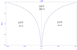
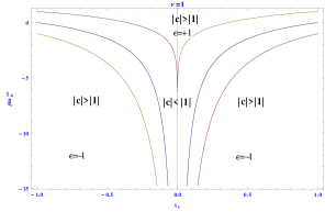
For what values of the bosonic Lagrangian parameters does this simplification happen? In order to answer this question we need to solve for $c_{B}$ as a function of Lagrangian parameters and then constrain these parameters using the inequalities above. We have implemented this procedure numerically on Mathematica at three different values of the chemical potential, $\nu_{B}=0$, $\nu_{B}=\frac{1}{2}$ and $\nu_{B}=1$. For each value of the chemical potential we have analyzed when (111) is obeyed on a graph whose $y$ axis is $\hat{m}_{B}^{\text{cri}}$ and whose $x$ axis is $\lambda_{B}$ in Fig 1,1,1.

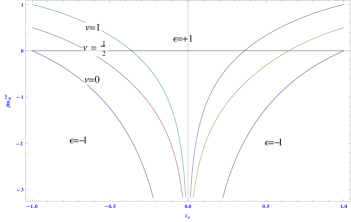
On intuitive grounds we expect the scalar to show an increasing tendency to condense at larger values of $|\nu_{B}|$ and at increasingly negative values of $m_{B}^{\text{cri}}$ (when the scalar field theory is increasingly tachyonic). We also expect finite temperature condensation to be forbidden by the Mermin Wagner theorem at $\lambda_{B}=0$. Our explicit results are in perfect agreement with this intuition. We find that the conditions listed in (113) are met provided we lie ‘above’ the highest curves in this plots given in Fig 1,1,1.333333In each of these plots the first condition in (113), ($|c_{B}|>|\nu_{B}|$) is met if we lie either above the highest curves on the plot or below the lowest curves on that plot. However the second condition in (113), namely $\epsilon>0$, is met only above the highest curves. Note that, on each of these plots, increasingly negative values of $m_{B}^{\text{cri}}$ and increasingly large values of $|\nu_{B}|$ tend to cause condensation. Note also that condensation becomes increasingly unlikely at small $\lambda_{B}$ and never occurs at $\lambda_{B}=0$. In Fig. 2 have replotted the highest curves of Figs. Fig 1,1,1 on the same graph for comparison. Note that the curve rises as $|\nu_{B}|$ is increased. This observation supports the intuition that increasing $|\nu_{B}|$ increases the probability of “condensation”. All in all our results qualitatively support the guess that the bosonic field Bose condenses when either of the inequalities in (113) are violated.

B.3 Dualization of the bosonic gap equation

In this subsection we demonstrate that no solution exists to the critical boson theory when the (dual of) the inequality $\text{sgn}(\lambda)c_{F}>0$ is violated.

The gap equation of the critical boson theory is

$$\begin{split}2\lambda_{B}{\cal S}&=\lambda_{B}m_{B}^{\text{cri}}.\\ \end{split}$$ (114)

We can rewrite this equation in fermionic dual variables as

$$\text{sgn}(\lambda_{F}){\rm max}\left(|{c_{F}}|,|\nu_{F}|\right)=\left(2\lambda_{F}{\cal C}+m_{F}^{\text{reg}}\right).$$ (115)

By comparing the signs of the RHS and LHS of this equation, it follows immediately that the equation has no solution unless

$$\text{sgn}\left(\lambda_{F}\left(2\lambda_{F}{\cal C}+m_{F}^{\text{reg}}\right)\right)>0$$ (116)

as we set out to show.

When this inequality is obeyed and $|{c_{F}}|>|\nu_{F}|.$ it follows that

$$\begin{split}\text{sgn}(\lambda_{F})|{c_{F}}|&=\left(2\lambda_{F}{\cal C}+m_{F}^{\text{reg}}\right)\\ |{c_{F}}|&=\text{sgn}(\lambda_{F})\left(2\lambda_{F}{\cal C}+m_{F}^{\text{reg}}\right).\end{split}$$ (117)

This is the fermionic gap equation. Note that (114) may have solutions when (116) is obeyed but $c_{B}<\nu_{B}$.

References

  • [1] J. Frohlich and T. Kerler, Universality in quantum Hall systems, Nucl.Phys. B354 (1991) 369–417.
  • [2] J. Frohlich and A. Zee, Large scale physics of the quantum Hall fluid, Nucl.Phys. B364 (1991) 517–540.
  • [3] E. Witten, Quantum Field Theory and the Jones Polynomial, Commun.Math.Phys. 121 (1989) 351.
  • [4] O. Aharony, O. Bergman, D. L. Jafferis, and J. Maldacena, N=6 superconformal Chern-Simons-matter theories, M2-branes and their gravity duals, JHEP 0810 (2008) 091, [arXiv:0806.1218].
  • [5] S. Giombi, S. Minwalla, S. Prakash, S. P. Trivedi, S. R. Wadia, et. al., Chern-Simons Theory with Vector Fermion Matter, Eur.Phys.J. C72 (2012) 2112, [arXiv:1110.4386].
  • [6] O. Aharony, G. Gur-Ari, and R. Yacoby, d=3 Bosonic Vector Models Coupled to Chern-Simons Gauge Theories, JHEP 1203 (2012) 037, [arXiv:1110.4382].
  • [7] J. Maldacena and A. Zhiboedov, Constraining Conformal Field Theories with A Higher Spin Symmetry, arXiv:1112.1016.
  • [8] J. Maldacena and A. Zhiboedov, Constraining conformal field theories with a slightly broken higher spin symmetry, arXiv:1204.3882.
  • [9] O. Aharony, G. Gur-Ari, and R. Yacoby, Correlation Functions of Large N Chern-Simons-Matter Theories and Bosonization in Three Dimensions, arXiv:1207.4593.
  • [10] S. Jain, S. P. Trivedi, S. R. Wadia, and S. Yokoyama, Supersymmetric Chern-Simons Theories with Vector Matter, JHEP 1210 (2012) 194, [arXiv:1207.4750].
  • [11] S. Yokoyama, Chern-Simons-Fermion Vector Model with Chemical Potential, arXiv:1210.4109.
  • [12] S. Giombi and X. Yin, The Higher Spin/Vector Model Duality, arXiv:1208.4036.
  • [13] O. Aharony, S. Giombi, G. Gur-Ari, J. Maldacena, and R. Yacoby, The Thermal Free Energy in Large N Chern-Simons-Matter Theories, arXiv:1211.4843.
  • [14] G. Gur-Ari and R. Yacoby, Correlators of Large N Fermionic Chern-Simons Vector Models, arXiv:1211.1866.
  • [15] S. Jain, S. Minwalla, T. Sharma, T. Takimi, S. R. Wadia, et. al., Phases of large $N$ vector Chern-Simons theories on $S^{2}\times S^{1}$, arXiv:1301.6169.
  • [16] T. Takimi, Duality and Higher Temperature Phases of Large $N$ Chern-Simons Matter Theories on $S^{2}\times S^{1}$, arXiv:1304.3725.
  • [17] C.-M. Chang, S. Minwalla, T. Sharma, and X. Yin, ABJ Triality: from Higher Spin Fields to Strings, arXiv:1207.4485.
  • [18] R. D. Pisarski and S. Rao, Topologically Massive Chromodynamics in the Perturbative Regime, Phys.Rev. D32 (1985) 2081.
  • [19] W. Chen, G. W. Semenoff, and Y.-S. Wu, Two loop analysis of nonAbelian Chern-Simons theory, Phys.Rev. D46 (1992) 5521–5539, [hep-th/9209005].
  • [20] A. Giveon and D. Kutasov, Seiberg Duality in Chern-Simons Theory, Nucl. Phys. B812 (2009) 1–11, [arXiv:0808.0360].
  • [21] F. Benini, C. Closset, and S. Cremonesi, Comments on 3d Seiberg-like dualities, JHEP 1110 (2011) 075, [arXiv:1108.5373].