Measurements and simulation of Faraday rotation across the Coma radio relic

Abstract

The aim of this work is to probe the magnetic field properties in relics and infall regions of galaxy clusters using Faraday Rotation Measures. We present Very Large Array multi-frequency observations of seven sources in the region South-West of the Coma cluster, where the infalling group NGC4839 and the relic 1253+275 are located. The Faraday Rotation Measure maps for the observed sources are derived and analysed to study the magnetic field in the South-West region of Coma. We discuss how to interpret the data by comparing observed and mock rotation measures maps that are produced simulating different 3-dimensional magnetic field models. The magnetic field model that gives the best fit to the Coma central region underestimates the rotation measure in the South-West region by a factor $\sim$6, and no significant jump in the rotation measure data is found at the position of the relic. We explore different possibilities to reconcile observed and mock rotation measure trends, and conclude that an amplification of the magnetic field along the South-West sector is the most plausible solution. Our data together with recent X-ray estimates of the gas density obtained with Suzaku suggest that a magnetic field amplification by a factor $\sim$3 is required throughout the entire South-West region in order to reconcile real and mock rotation measures trends. The magnetic field in the relic region is inferred to be $\sim 2\,\mu$G, consistent with Inverse Compton limits.

1 Introduction

The hot and rarefied plasma that fills the intra-cluster medium (ICM) of galaxy clusters is known to be magnetised. The existence of the magnetic field in galaxy clusters is inferred from radio observations of radio halos and relics, which are synchrotron emitting sources not obviously connected to any of the cluster radio galaxies. Nowadays, this emission is detected in $\sim$ 70 objects (Feretti et al., 2012). Radio relics are diffuse extended radio sources in the outer regions of galaxy clusters. The radio emission indicates the presence of relativistic particles and magnetic fields (see reviews by Brüggen et al., 2011, and references therein). The origin of relics is still uncertain: there is a general consensus that it is related to shock waves occurring in the ICM during merging events. Cosmological simulations indicate that shock waves are common phenomena during the process of structure formation, and the Mach numbers of merging shocks are expected to be of the order of $\sim$ 2-4 (e.g. Skillman et al., 2008, 2012; Vazza et al., 2010, 2011; Kang & Ryu, 2011; Ryu et al., 2003). However, the direct detection of shock waves is difficult, because of the low X-ray surface brightness of the clusters at their periphery. So far, only a handful of shock fronts have been unambiguously detected through both a temperature and a surface brightness jump: the “bullet cluster” - 1E 065756 - (Markevitch et al., 2002), Abell 520 (Markevitch et al., 2005), Abell 3667 (Finoguenov et al., 2010; Akamatsu & Kawahara, 2013), Abell 2146 (Russell et al., 2011), Abell 754 (Macario et al., 2011), CIZAJ2242.8+5301 (Akamatsu & Kawahara, 2013; Ogrean et al., 2013), and Abell 3376 (Akamatsu & Kawahara, 2013). Among these clusters, Abell 3667, CIZAJ2242.8+5301, Abell 754, and Abell 3376 host one or two radio relics, a radio halo is found in the bullet cluster and in Abell 520, while no radio emission is detected in Abell 2146. Hence, there is not always a one-to-one connection between a radio relic and a shock wave detected through X-ray observations. In addition, the mechanism responsible for the particle acceleration is not fully understood yet. Shock waves should amplify the magnetic field and (re)accelerate protons and electrons to relativistic energies, producing detectable synchrotron emission in the radio domain (Ensslin et al., 1998; Iapichino & Brüggen, 2012). The process responsible for the particle acceleration could be either direct Diffusive Shock Acceleration or shock re-acceleration of previously accelerated particles (e.g. Hoeft & Brüggen, 2007; Macario et al., 2011; Kang et al., 2012; Kang & Ryu, 2011). Regardless of the origin of the emitting relativistic electrons, a key role is played by the magnetic field. Previous magnetic field estimates in radio relics have been obtained using three different approaches:

• radio equipartition arguments, resulting in magnetic field estimates of $\sim 1\;\mu\rm{G}$ (see e.g. review by Feretti et al., 2012).
  

• Inverse Compton (IC) studies, resulting mostly in lower limits on the magnetic field strength $>1\;\mu\rm{G}$ (see Chen et al., 2008, and references therein).
  

• Width of the relic, as proposed by Hoeft & Brüggen (2007)- only applied so far by van Weeren et al. (2010)- resulting in magnetic field estimates of $0.2-7\mu\rm{G}$. This technique assumes that a shock wave is present at the location of the observed radio emission.

Equipartition estimates rely on several assumptions that are difficult to verify. IC emission is hardly detected from radio relics, hence leading mostly to average lower limits for the magnetic field strength. The method proposed by Hoeft & Brüggen (2007) can be applied only in particular circumstances (see van Weeren et al., 2010, for details).
Another method to analyse the magnetic field is the study of the Faraday Rotation. The interaction of the ICM, a magneto-ionic medium, with the linearly polarized synchrotron emission results in a rotation of the wave polarization plane (Faraday Rotation), so that the observed polarization angle, $\Psi_{\rm obs}$ at a wavelength $\lambda$ differs from the intrinsic one, $\Psi_{\rm int}$ according to:

$$\Psi_{\rm obs}(\lambda)=\Psi_{\rm int}+\lambda^{2}\times RM,$$ (1)

where RM is the Faraday Rotation Measure. This is related to the magnetic field component along the line-of-sight ($B_{//}$) weighted by the electron number density ($n_{e}$) according to:

$$RM\propto\int_{los}n_{e}(l)B_{//}(l)dl.$$ (2)

Statistical RM studies of clusters and background sources show that magnetic fields are common in both merging and relaxed clusters (Clarke, 2004; Johnston-Hollitt et al., 2004), although their origin and evolution are still uncertain. Information about the magnetic field strength, radial profile and power spectrum can be obtained by analyzing the RM of sources located at different distances from the cluster center (see e.g. Murgia et al., 2004; Govoni et al., 2006; Guidetti et al., 2008; Bonafede et al., 2010; Govoni et al., 2010). These studies indicate that the magnetic field strength decreases from the center to the periphery of the cluster in agreement with predictions from cosmological simulations (e.g. Dolag et al., 1999; Brüggen et al., 2005; Dolag & Stasyszyn, 2009; Ruszkowski et al., 2011; Bonafede et al., 2011b). Observations and simulation indicate that the magnetic field in cluster outskirts is a fraction of $\mu\rm{G}$. So far, the RM method has not been applied to relics and infall regions, but only to the central regions of a few galaxy clusters. This is partly due to the difficulty of finding several sources - located in projection through the region that one wants to analyse - that are both extended and sufficiently strong to derive the RM distribution with the desired accuracy.
In this work, we investigate the magnetic field strength and topology in the region of the relic in the Coma cluster using RM analysis of sources located in the region of the relic. The relic in the Coma cluster is among the best candidates for this kind of study: it has a large angular extent ($\sim$ 0.5^∘), hence some radio sources are seen in projection through it; it was the first relic that was discovered, making it one of the most studied, and often the test-case for theoretical models (e.g. Ensslin et al., 1998); in addition, recent radio (Brown & Rudnick, 2011) and X-ray (Ogrean & Brüggen, 2012; Akamatsu et al., 2013; Simionescu et al., 2013) observations suggest the presence of a long filamentary structure South-West of the Coma cluster, associated with the NGC4839 group and with the relic. Ogrean & Brüggen (2012) and Akamatsu et al. (2013) found a possible $M\sim 2$ shock, in a region spatially coincident with the relic, although such a shock has been detected only in temperature and not in density or surface brightness. Finally, previous studies of Coma have already set constraints on the magnetic field strength and structure of the cluster (Bonafede et al., 2010). In Bonafede et al. (2010), we have studied the Faraday RM of several sources located in the Coma cluster, excluding the South-West region where the infall group is located. Through a comparison with mock RM images, we have derived the magnetic field model which best reproduces the observed RMs within the central 1.5 Mpc region. The best agreement with data is achieved with a magnetic field central strength of 4.7 $\mu$G, and a radial slope that follows the square-root of gas density profile. Starting from these results, it is possible to estimate whether a magnetic field amplification is required in the relic region. An overview of the sources’s position with respect to the Coma cluster is displayed in Fig. 1.
The paper is organised as follows: radio observations and data reduction are reported in Sec. 2, and the results of the Faraday RM are reported in Sec. 3. In Sec. 4 we describe the technique we use to produce mock RM observations, and in Sec. 5 mock and observed RM images are analysed and compared . Our results are discussed in Sec. 6 and finally, we conclude in Sec. 7.
Throughout this paper,s we assume a concordance cosmological model $\rm{\Lambda CDM}$, with $H_{0}=$ 71 km s^-1 Mpc^-1, $\Omega_{M}=$ 0.27, and $\Omega_{\Lambda}=$ 0.73. One arcsec corresponds to 0.46 kpc at $z=$0.023.

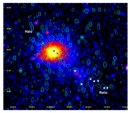
Figure 1: Colours: X-ray emission from the Coma cluster and the NGC4839 group from the Rosat All Sky Survey (Briel et al., 1992). Contours: Radio emission from WSRT at 325 MHz (Venturi et al., 1990). Contours level are at 0.3, 1 and 3 mJy/beam. The beam is $\sim 50"\times 125"$. Crosses mark the position of the sources in the Coma cluster (green and red) and in the NGC4839 group (white crosses), analysed in this work.

2 Radio observations

2.1 VLA observations and data reduction

From the FIRST survey (Becker et al., 1995), we selected the 6 brightest and extended radio galaxies that appeared in the NVSS to be polarised (Condon et al., 1998). Three of them are well-known Coma radio galaxies: 5C4.51, the central galaxy of the merging group referred by us as the NGC 4839 group, 5C4.43, and 5C4.20. The other radio-sources are background objects. In the field of view of 5C4.20 another source was found to be unresolved and polarised: 5C4.16, which has been included in our analysis. Observations were carried out at the VLA using the 6 cm and 20 cm bands. The 20 cm observations were performed in the B array configuration, with 25 MHz bandwidth, while the 6 cm observations were performed in the C array configuration, with 50 MHz bandwidth. The sources were observed at two frequencies within each band in order to obtain adequate coverage in $\lambda^{2}$ and determine the RM unambiguously. This setup allows one to have the same UV-coverage in both bands and offers the best compromise between resolution and sensitivity to the sources’ extended structure. The resulting angular resolution of $\sim$4^′′ corresponds to $\sim$ 2 kpc at the cluster’s redshift. Having a high resolution is crucial to determine small-scale RM fluctuations. At the same time, we also need good sensitivity to the extended emission, in order to image RM variations on the largest scales. The largest angular scale (LAS) visible in the 20-cm band with the B array is 120^′′. From NVSS the sources 5C4.20 and 5C4.43 have a larger angular extent, hence we also observed them with C array configuration. Details of the observations are given in Table 1. Since observations were taken in the VLA-EVLA transition period, baseline calibration was performed, using the source 1310+323 as calibrator. The source 3C286 was used as both primary flux density calibrator and as absolute reference for the electric vector polarisation angle. The source 1310+323 was observed as both a phase and parallactic angle calibrator.
We performed standard calibration and imaging using the NRAO Astronomical Imaging Processing Systems (AIPS). Cycles of phase self-calibration were performed to refine antenna phase solutions on target sources, followed by a final amplitude and gain self-calibration cycle in order to remove minor residual gain variations. Total intensity, I, and Stokes parameter Q and U images have been obtained for each frequency separately. The final images were then convolved with a Gaussian beam having FWHM $=$ 5${}^{\prime\prime}\times$5^′′ ($\sim$ 2.3$\times$2.3 kpc). Polarization intensity $P=\sqrt{U^{2}+Q^{2}}$, polarization angle $\Psi=\frac{1}{2}\operatorname{atan}(U,Q)$ and fractional polarization $FPOL=\frac{P}{I}$ images were obtained from the I, Q and U images. Polarization intensity images have been corrected for a positive bias. The calibration errors on the measured fluxes are estimated to be $\sim$ 5%.

Table 1: VLA observations of radio galaxies in the Coma cluster field.

Source	RA	DEC	$\nu$	Bandwidth	Config.	Date	Net Time on Source
	(J2000)	(J2000)	(GHz)	(MHz)			(Hours)
5C4.20	12 54 18.8	+27 04 13	4.535 - 4.935	50	C	Jul 09	3.0
			1.485 - 1.665	25	B	May 09	1.6
			1.485 - 1.665	25	C	Jul 09	1.6
5C4.24	12 54 58.9	+27 14 51	4.535 - 4.935	50	C	Jul 09	3.5
			1.485 - 1.665	25	B	May 09	2.0
5C4.29	12 55 21.0	+27 14 44	4.535 - 4.935	50	C	Jul 09	3.0
			1.485 - 1.665	25	B	May 09	2.0
5C4.31	12 55 43.3	+27 16 32	4.535 - 4.935	50	C	Jul 09	3.2
			1.485 - 1.665	25	B	Apr - May 09	3.2
5C4.43	12 56 43.6	+27 10 41	4.535 - 4.935	50	C	Jul 09	3.0
			1.485 - 1.665	25	B	Apr - May 09	2.8
			1.485 - 1.665	25	C	Jul 09	1.6
5C4.51	12 57 24.3	+27 29 51	4.535 - 4.935	50	C	Jul 09	3.0
			1.485 - 1.665	25	B	May 09	3.2
Col. 1: Source name; Col. 2, Col. 3: Pointing position (RA, DEC); Col. 4: Observing frequency;
Col 5: Observing bandwidth; Col. 6: VLA configuration; Col. 7: Dates of observation;
Col. 8: Time on source (flags taken into account).

Table 2: Total and polarization intensity radio images. Images are restored with a beam of 5${}^{\prime\prime}\times$5^′′

Source name	$\nu$	$\sigma$(I)	$\sigma$(Q)	$\sigma$(U)	Peak brightness	Flux density	Pol. flux
	(GHz)	(mJy/beam)	(mJy/beam)	(mJy/beam)	(mJy/beam)	(mJy)	(mJy)
5C4.20	1.485	0.050	0.024	0.024	9.0206E-03	8.1052E-02	1.6721E-02
	1.665	0.059	0.026	0.026	9.2810E-03	8.0599E-02	1.7609E-02
	4.535	0.020	0.017	0.017	5.5346E-03	4.0829E-02	8.8433E-03
	4.935	0.019	0.018	0.018	5.5642E-03	4.1919E-02	8.8699E-03
5C4.16	1.485	0.050	0.024	0.024	2.1867E-02	4.2672E-02	2.7042E-03
	1.665	0.059	0.026	0.026	2.1905E-02	3.9896E-02	2.7011E-03
	4.535	0.020	0.017	0.017	6.3046E-03	1.1521E-02	8.2612E-04
	4.935	0.019	0.018	0.018	5.7240E-03	1.1033E-02	7.0368E-04
5C4.24	1.485	0.048	0.025	0.024	8.3123E-03	3.4E-02	1.4087E-03
	1.665	0.049	0.029	0.028	9.726E-04	2.8395E-02	1.8146E-03
	4.535	0.018	0.017	0.016	4.4992E-03	1.4653E-02	1.7374E-03
	4.935	0.017	0.017	0.017	4.4218E-03	1.3855E-02	1.3685E-03
5C4.29	1.485	0.049	0.023	0.023	3.9605E-03	1.6574E-02	7.4013E-04
	1.665	0.049	0.028	0.028	3.6253E-03	1.3414E-02	5.5392E-04
	4.535	0.018	0.017	0.017	2.7847E-03	6.2474E-03	1.9849E-04
	4.935	0.018	0.018	0.017	2.7966E-03	5.1822E-03	1.9345E-04
5C4.31	1.485	0.047	0.017	0.017	7.4910E-03	1.9235E-02	1.9059E-03
	1.665	0.046	0.023	0.022	7.6109E-03	1.9606E-02	1.8874E-03
	4.535	0.017	0.017	0.017	2.9999E-03	7.1626E-03	5.9231E-04
	4.935	0.018	0.017	0.017	2.9737E-03	7.2758E-03	5.9357E-04
5C4.43	1.485	0.045	0.019	0.021	8.5986E-03	5.0856E-02	7.2086E-03
	1.665	0.041	0.023	0.023	8.6323E-03	4.5734E-02	7.2029E-03
	4.535	0.015	0.013	0.013	6.1534E-03	2.5576E-02	3.0802E-03
	4.935	0.015	0.013	0.014	6.2770E-03	2.5461E-02	2.8089E-03
5C4.51	1.485	0.051	0.022	0.021	8.3728E-03	6.6565E-02	4.1651E-03
	1.665	0.058	0.024	0.024	8.1401E-03	6.4310E-02	4.0893E-03
	4.535	0.018	0.017	0.017	3.8679E-03	2.7415E-02	2.1236E-03
	4.935	0.018	0.017	0.018	3.6772E-03	2.5692E-02	2.0066E-03
Col. 1: Source name; Col. 2: Observation frequency; Col. 3, 4, 5: RMS noise of the I, Q, U images;
Col. 7: Peak brightness; Col. 8: Flux density; Col. 9: Polarized flux density.

2.2 Radio properties of the observed sources

In this section the radio properties of the observed sources are briefly presented. Further details are given in Table 2.
Redshift information is available for three out of the seven radio sources. Although the redshift is not known for the other four radio sources, they have not been associated with any cluster galaxy down to very faint optical magnitudes: M${}_{r}\geq$ -15 (see Miller et al. 2009). This indicates that they are background radio sources, seen in projection through the radio relic. In the following, the radio emission arising from the selected sample of sources is described together with their main polarisation properties.

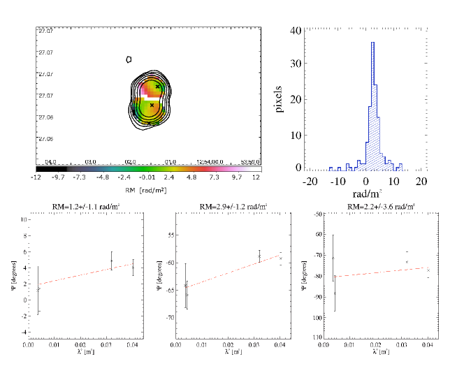
Figure 3: 5C4.16: Top left: The RM image is shown in color along with total intensity radio contours at 1.4 GHz. Contours start at 3$\sigma$ and increase by factors of 2. Top right: distribution histogram of the RM values. Bottom: fits of polarisation angle versus $\lambda^{2}$ in three representative pixels marked with crosses in the top-left image.

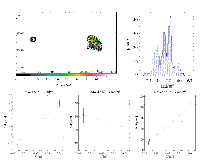
Figure 4: 5C4.24: Top left: The RM image is shown in colour along with total intensity radio contours at 1.4 GHz. Contours start at 3$\sigma$ and increase by factors of 2. Top right: distribution histogram of the RM values. Bottom: fits of polarisation angle versus $\lambda^{2}$ in three representative pixels marked with crosses in the top-left image.

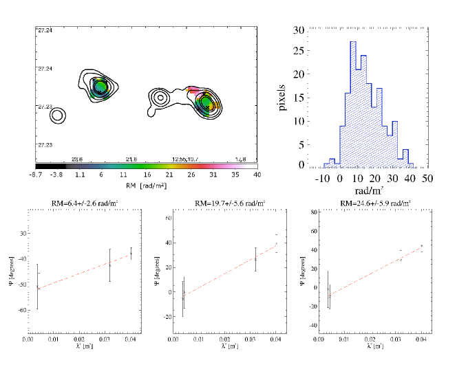
Figure 5: 5C4.29: Top left: The RM image is shown in colours along with total intensity radio contours at 1.4 GHz. Contours start at 3$\sigma$ and increase by factors of 2. Top right: distribution histogram of the RM values. Bottom: fits of polarisation angle versus $\lambda^{2}$ in three representative pixels marked with crosses in the top-left image.

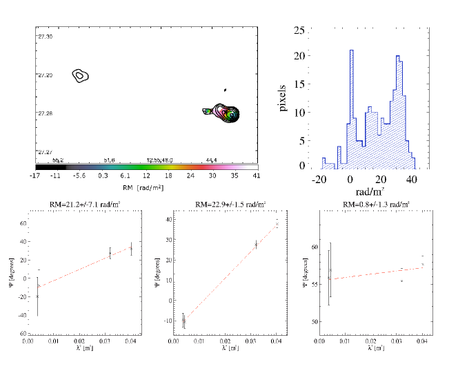
Figure 6: 5C4.31: Top left: The RM image is shown in colour along with total intensity radio contours at 1.4 GHz. Contours start at 3$\sigma$ and increase by factors of 2. Top right: distribution histogram of the RM values. Bottom: fits of polarisation angle versus $\lambda^{2}$ in three representative pixels marked with crosses in the top-left image.

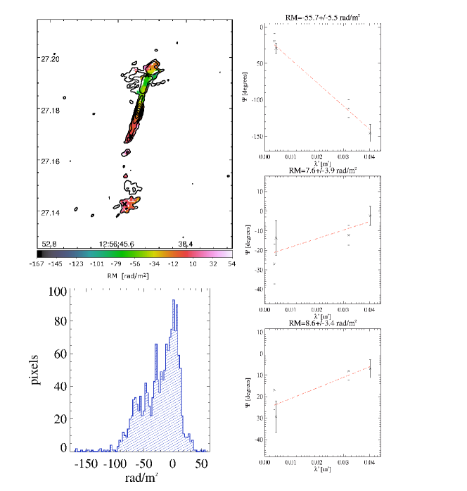
Figure 7: 5C4.43: Left top: The RM image is shown in colour along with total intensity radio contours at 1.4 GHz. Contours start at 3$\sigma$ and increase by factors of 2. Left bottom: distribution histogram of the RM values. Right: fits of polarisation angle versus $\lambda^{2}$ in three representative pixels marked with crosses in the left-top image.

5C4.20 - NGC 4789
The radio emission of NGC 4789 is associated with an elliptical galaxy with an apparent optical diameter of $\sim$ 1^′.7 located at redshift z$\sim$0.028 (De Vacoulers et al. 1976). It lies at $\sim 1.5^{\circ}$ from the cluster centre, South-West of the Coma relic. The radio source is characterised by a Narrow Angle Tail (NAT) structure. In our high-resolution images the source shows two symmetric and collimated jets that propagate linearly from the centre for $\sim 35^{\prime\prime}$ in the SE- NW direction (see Fig. 2). Then, the jets start bending toward North-East up to a linear distance of $\sim 130^{\prime\prime}$ from the galaxy. The brightness decreases from the centre of the jets towards the lobes that appear more extended in the 20-cm band images. On average the source is polarised at the 20% level at 1.485 GHz and at the 24% level at 4.935 GHz. Lower resolution images by Venturi et al. (1989) show that the total extent of the source is $\sim 6^{\prime}$, from the core to the outermost low-brightness features. Venturi et al. (1989) also note that no extended lobes are present at the edges of the jets, and the morphology of the low brightness regions keeps following the jets’ direction without transverse expansion.
5C4.16
Another source is located 3^′.8 West of 5C4.20. It is 5C4.16 (Fig. 3). 5C4.16 is moderately extended, with a LLS of $\sim$20^′′, but enough to be resolved by more synthesised beams. 5C4.16 is also polarised: 7% on average at both 1.485 GHz and 5.985 GHz. Hence, although this source was not the target of the observation, it adds a piece of information to our analysis.
5C4.24
The radio emission from the source is likely associated with the lobe of a radio galaxy centred on RA$=$12h55m08.3s and DEC$=$+27d15m34s (see Fig. 4). The redshift of the source is $z=$0.257325, according to McMahon et al. (2002). Hence, 5C4.24 lies in the background of the Coma cluster and is projected onto the radio relic. In our images, we detect the nucleus, the lobe and a weak counter-lobe (which is not shown in Fig. 4). The projected position of 5C4.24 is at $\sim 1.2^{\circ}$ from the Coma cluster centre. The emission from the counter-lobe is too weak to be detected in polarisation. However, the lobe shows a mean fractional polarisation of 8% at 1.485 GHz, which increases to 13% at 4.935 GHz.
5C4.29
5C4.29 is located at $\sim 1.2^{\circ}$ from the centre of the Coma cluster. Three distinct components are visible in our images (Fig. 5). A nucleus and two bright lobes are detected from 1.485 GHz to 4.935 GHz. The western lobe is connected to the nucleus through a region of lower brightness, visible only in the 20-cm band images. No redshift is available for this radio-source. Its total extension is $\sim 68^{\prime\prime}$. We note that if the source was located at the Coma redshift, this would translate into a linear size of 31 kpc, that would be exceptionally small for a radio-galaxy. The western lobe is polarised on average at the 7% level at both 1.485 GHz and 4.935 GHz, while the eastern lobe is polarised at 5% and 8% at 1.485 GHz and 4.935 GHz respectively.
5C4.31
Our images suggest that the source 5C4.31 is associated with the brightest lobe of a radio galaxy (see Fig. 6). A weaker counter-lobe is also visible in our images, while the nucleus is only detected in the 6-cm band images. It is located in projection onto the radio relic, close to its eastern edge. The projected distance from the cluster centre is $\sim 1.1^{\circ}$. The lobe exhibits a mean fractional polarisation of $\sim$13% and 10% at 1.485 and 4.935 GHz, respectively.
5C4.43 - NGC 4827
The radio emission from 5C4.43 is associated with the elliptical galaxy NGC4827 at z$=$ 0.025 (Smith et al., 2000). It is located in-between the Coma cluster and the radio relic, at $\sim 1^{\circ}$ from the cluster centre. The radio source was studied in detail by Venturi et al. (1989): it has a Z-shaped morphology with some evidence of jets joining the core of the radio source to the diffuse emission of the lobes. The angular extent of the source at 1.4 GHz is $\sim 4^{\prime}30^{\prime\prime}$ (Venturi et al., 1989). Our observations show the core and two bright jets departing in the N and S direction. The brightness of the jets decreases as they propagate out from the nucleus, and fade into two diffuse lobes (Fig. 7). The lobes appear more extended in our 20-cm band images. This is due to the steep spectrum that characterises the lobes or the radio-galaxies. Both, the jets and the diffuse lobes are polarised. We detect a mean polarisation of $\sim$10% at 1.485 GHz and 4.935 GHz.
5C4.51 - NGC 4839
The radio source 5C4.51 is identified with NGC 4839, the brightest galaxy of the group NGC 4839, which is currently merging with the Coma cluster. The redshift of the source is $\sim$ 0.25 (Smith et al., 2000). 5C4.51 is located at $\sim 0.6^{\circ}$ from the Coma cluster centre. The source largest extension is $\sim 1^{\prime}$, and it is composed of two extended and connected radio lobes, while the nucleus is not resolved. The source is polarised on average at the 7% and 9% level at 1.485 GHz and 4.935 GHz, respectively.

3 Rotation Measures

We derived the fit to the RMs from the polarisation angle images using the PACERMAN algorithm (Polarization Angle CorrEcting Rotation Measure ANalysis) developed by Dolag et al. (2005b). The algorithm uses a few selected reference pixels to solve for the n$\pi$-ambiguity in a nearby area of the map. Once the n$\pi$-ambiguity is solved for, the RMs can be computed also in low signal-to-noise regions. As reference pixels we considered those with a polarisation angle uncertainty of less than 10 degrees, corresponding to 2$\sigma$ level in both U and Q polarisation maps simultaneously. The n$\pi$ value found for the reference pixel is then transferred to the nearby pixels, if their polarisation angle gradient is below a certain threshold at all frequencies. We fixed this threshold to 15 to 25 degrees, depending on the image features. The resulting RM images are shown in Fig. 2, 3, 4, 5, 6, 7, and 8 overlaid onto the total intensity contours at 1.485 GHz. In the same figures, we also display the RM distribution histograms and the RM fits for some representative pixels, marked by crosses in the respective images.
The polarisation angle $\Psi$ follows the $\lambda^{2}$-law, expected in the case of an external Faraday screen. We will assume in the following that the Faraday Rotation is occurring entirely in the ICM and it is hence representative of the magnetic field weighted by the gas density of the cluster. We will discuss this assumption in Sec. 3.3.
From the RM images, we computed the RM mean ($\langle\rm RM\rangle$) and its dispersion ($\sigma_{\rm{RM,obs}}$) (see Table 3).

Table 3: Rotation Measure values of the observed sources

Source	Proj. distance	n. of beams	$\langle RM\rangle$	$\sigma_{\rm{RM}}$	Errfit
	kpc		rad/m2	rad/m2	rad/m2
5C4.20	2451	62	4.8 $\pm$0.7	5.2$\pm$0.6	2.9
5C4.16	2543	5	2.8 $\pm$2	3.3$\pm$1.5	1.5
5C4.24	2075	16	13 $\pm$4	15 $\pm$3	4.3
5C4.29	1982	7	15 $\pm$4	10 $\pm$4	5.8
5C4.31	1824	8	18 $\pm$5	14 $\pm$4	3.2
5C4.43	1667	55	-22 $\pm$4	31 $\pm$3	5.5
5C4.51	1113	21	69 $\pm$ 9	43 $\pm$ 7	3.9
Col. 1: Source name Col. 2: Source projected distance from the X-ray cluster centre;
Col. 3: number of beams over which RMs are computed;
Col. 4: Mean value of the RM distribution;
Col. 5: Dispersion of the RM distribution;
Col. 6: Median of the RM fit error.

3.1 Errors on the RM

The errors that affect the values of $\langle\rm RM\rangle$ and $\sigma_{\rm{RM,obs}}$ can be separated into fit errors and statistical errors. The former has the effect of increasing the real value of $\sigma_{\rm{RM}}$, while the latest is due to the finite sampling of the RM distribution. In our case, it is determined by the number of beams, $n_{b}$, over which the RM is computed. In order to derive the real standard deviation of the observed RM distribution, we have computed the $\sigma_{\rm{RM}}$ as $\sqrt{\sigma^{2}_{\rm{RM,obs}}-\rm{Err}_{\rm{fit}}^{2}}$. $\rm{Err_{fit}}$ is the median of the error distribution, and $\sigma^{2}_{\rm{RM,obs}}$ is the observed value of the RM dispersion. Errors have been estimated with Monte Carlo simulations, following the same approach used in Bonafede et al. (2010). We have extracted $n_{b}$ values from a random Gaussian distribution having $\sigma=\sigma_{\rm{RM,obs}}$ and mean $=\langle\rm RM\rangle$. In order to mimic the effect of the noise in the observed RM images, we have added to the extracted values Gaussian noise having $\sigma_{\rm{noise}}=Err_{\rm{fit}}$. We have computed the mean and the dispersion ($\sigma_{\rm{sim}}$) of these simulated quantities and then subtracted the noise from the dispersion obtaining $\sigma_{\rm{sim,dec}}=\sqrt{\sigma_{\rm{sim}}^{2}-\sigma_{\rm{noise}}^{2}}$. Thus, we have obtained a distribution of $\sigma_{\rm{sim,dec}}$ and means. The standard deviation of the $\sigma_{\rm{sim,dec}}$ distribution is then assumed to be the uncertainty on $\sigma_{\rm{RM,dec}}$, while the standard deviation of the mean distribution is assumed to be the fit error on $\langle RM\rangle$. We checked that the mean of both distributions recover the corresponding observed values. In Table 3 we list the RM mean, its dispersion ($\sigma_{\rm{RM}}$), with the respective errors, the median of the fit error ($\rm{Err}_{\rm{fit}}$), and the number of beams over which the RM statistic is computed ($n_{b}$).

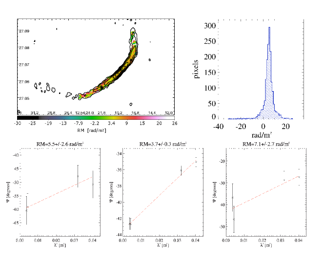
Figure 2: 5C4.20: Top left: The RM fit is shown in colour along with total intensity radio contours 1.4 GHz. The bottom contour correspond to the 3$\sigma$ noise level and contours are then spaced by a factor of 2. Top right: distribution histogram of the RM values. Bottom: fits of polarisation angle versus $\lambda^{2}$ in three representative pixels marked with crosses in the top-left image.

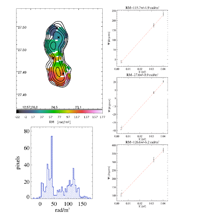
Figure 8: 5C4.51: Left top: The RM image is shown in colour along with total intensity radio contours at 1.4 GHz. Contours start at 3$\sigma$ and increase by factors of 2. Left bottom: distribution histogram of the RM values. Right: fits of polarisation angle versus $\lambda^{2}$ in three representative pixels marked with crosses in the left-top image.

3.2 Galactic contribution

The contribution to the Faraday RM from our Galaxy may introduce an offset in the Faraday rotation that must be removed. This contribution depends on the Galactic positions of the observed sources. The Galactic coordinates of the Coma cluster are $l=58^{\circ}$ and $b=88^{\circ}$. The cluster is close to the Galactic north pole, so that Galactic contribution to the observed RM is likely negligible. We have estimated the Galactic contribution as in Bonafede et al. (2010). Using the catalogue by Simard-Normandin et al. (1981), the average contribution for extragalactic sources located in projection close to the Coma cluster is $\sim$ -0.15 rad/m² in a region of 25$\times$25 degrees² centered on the cluster (The RM from each source has been weighted by the inverse of the distance from the centre of the Coma cluster). This small contribution is negligible and will not be considered in the following analysis.

3.3 RM local contribution

Here we discuss the possibility that the RMs observed in radio galaxies are not associated with the foreground ICM but may arise locally to the radio source (Bicknell et al. 1990, Rudnick & Blundell 2003, see however Ensslin et al. 2003), either in a thin layer of dense warm gas mixed along the edge of the radio emitting plasma, or in its immediate surroundings. Recently, Guidetti et al. (2012) and O’Sullivan et al. (2013) have found a local contribution to the RM in the lobes of B2 0755+37 and CentaurusA smaller than 20 rad/m², much smaller than the values measured in the Coma radiogalaxies analysed in Bonafede et al. (2010). This fact and the clear trend with the cluster projected distance indicate that the RM is due to the ICM rather than to local effectss. Although a local contribution cannot be rejected, it is unlikely to be dominating over the cluster ICM contribution. In addition, the RM map of B2 0755+37 shows stripes and gradients on the scales of the lobes that are pointing towards the presence of a local compression, while we do not detect any of such structures for the Coma cluster sources. We speculate that if a local contribution was produced by compressed gas and field around the leading edges of the lobes, and if such contribution was the dominant one, then RM stripes or gradient on scales as large as the lobes should be detected in the RM map. Additional statistical arguments against a local contribution are:

• A trend of the RM versus the cluster impact parameter has been observed (Clarke, 2004; Feretti et al., 1999; Govoni et al., 2006; Bonafede et al., 2011a, e.g.);
  

• Statistical tests on the scatter plot of RM versus polarisation angle for several radio galaxies show that no evidence is found for a Faraday rotation local to radio lobes.(Ensslin et al., 2003);
  

• The relation between the maximum RM and the cooling flow rate in relaxed clusters (Taylor et al., 2002) indicates that the RM of cluster sources is sensitive to the cluster environment rather than to the lobe internal gas.
  

Among the sources analysed in this paper, only 3 belong to the Coma cluster or NGC4839 group (namely, 5C4.20, 5C4.43, and 5C4.51), while the other 4 are field sources in the background of the cluster. Since there is no evidence for a local contribution in the RM images that we are presenting in this work (Fig. 2 to 8), and the trend of $\Psi$ versus $\lambda^{2}$ follows the expectations for an external Faraday screen, we will assume that the RM we detect is originating entirely in the ICM.
The trend of $\langle|\rm{RM}|\rangle$ and $\sigma_{\rm RM}$ are shown in Fig. 9 for the new sources analysed in this work as well as for the sources located in the Coma cluster (Bonafede et al., 2010). The average trend indicates that the RM decreases from the centre towards the outskirts of the cluster, although an increment in both $\langle|\rm{RM}|\rangle$ and $\sigma_{\rm RM}$ is detected in the SW quadrant. A net increase of the $\langle|\rm{RM}|\rangle$ is detected corresponding to the central sources of the group NGC 4839 interacting with the Coma cluster. In the following sections we will analyse if the detected trend is compatible with the magnetic field profile derived from the Coma cluster, or if an additional component of either the magnetic field, B, and/or the gas density, $n$, is needed.

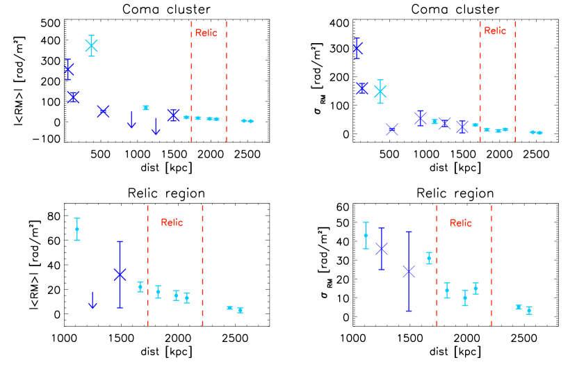
Figure 9: $\langle|\rm{RM}|\rangle$ and $\sigma_{\rm{RM}}$ trend versus the cluster projected distance. Crosses are the points from Bonafede et al. (2010), dots are the new points from this paper. Blue symbols mark the sources in the Coma cluster, cyan symbols mark those SW from the cluster centre, in the direction of the Coma relic. Red vertical lines indicate the approximative location of the Coma relic. In the top panels all the sources and displayed, in the bottom panels a zoom in the SW region is shown.

4 Reproducing RM images

In this Section we describe the steps implemented in our method to produce simulated trend of RM for galaxy clusters. The numerical procedures have been inspired by the work of Murgia et al. (2004). The detailed implementation and developments, written in IDL, will be subject of a forthcoming paper. We outline here the main features of the code.
First, it produces a synthetic model for the gas density. Second, it creates a 3D distribution of a magnetic field model from an analytical power spectrum within a fixed range of spatial scales, and scales it to follow a given radial profile (or to scale with gas density). Third, it computes the RMs to be compared with real data taking into account the real sampling of the observed maps.
In detail:
$\bullet$ Input gas density model. We impose a model for the gas density, like e.g. the $\beta$-model (Cavaliere & Fusco-Femiano, 1976) or a combination of $\beta$-models to reproduce non-isolated clusters. The input gas model could also be taken directly from cosmological numerical simulations, although we will not explore this in the present work.
$\bullet$ 3D cluster magnetic field. In order to set up divergence-free, turbulent magnetic fields, we start with the vector potential ${\bf A}$. In the Fourier domain, it is assumed to follow a power-law with index $m$ between the minimum and the maximum wavenumber $k_{\rm in}\leq k\leq k_{\rm out}$:

$$P_{\rm A}(k)=|\rm{A_{k}}|^{2}\propto k^{-m}.$$ (3)

For all grid points in Fourier space, we extract random values of amplitude and phase, corresponding to each component of $\bf{A_{k}}$. In order to obtain a random Gaussian distribution for ${\bf B}$, $\bf{A}$ is randomly drawn from the Rayleigh distribution:

$$P(A,\phi)dAd\phi=\frac{A}{2\pi|A_{k}|^{2}}\exp\left(-\frac{A^{2}}{2|A_{k}|^{2}}\right)\cdot dAd\phi,$$ (4)

while $\phi$ is uniformly distributed in the range $[0,2\pi]$. The combination of $A$ and $\phi$ allows us to compute the value of ${\bf{A_{k}}}$ for each point in the Fourier domain ($k_{x}$, $k_{y}$, $k_{z}$). The magnetic field components in the Fourier space are then obtained by computing the curl of ${\bf{A_{k}}}$ thus generated:

$${\bf{\tilde{B}}}(k)=i{\bf k}\times{\bf{A_{k}}}.$$ (5)

The field components $B_{i}$ in real space are then derived using a 3D Fast Fourier Transform.
The magnetic field generated in this way is by definition divergence-free, with Gaussian components $B_{i}$ having zero mean and a dispersion equal to $\sigma_{B_{i}}=\langle B^{2}_{i}\rangle$. The magnetic field power spectrum is described by a power law $|B_{k}|^{2}\propto k^{-m+2}$.
In order to simulate a realistic profile of cluster magnetic field, we need to scale $|{\bf B}|$ for the distribution of gas density in the ICM. This is done by multiplying the 3D cube obtained in the previous step for a function of the gas density, $F(n)$. Based on the results of Bonafede et al. (2010), we will assume in this work $F(n)\propto n^{0.5}$, which means that for an isothermal ICM the magnetic field energy density scales with the gas thermal energy, $B^{2}\propto nk_{\rm B}T$. We finally normalise our 3D distribution requiring that the average magnetic field inside a given radius (which is usually fixed to be cluster core radius) is $B_{0}$. The constant of normalisation is hence defined as:

$$\beta=\frac{B_{\rm 0}}{\frac{\displaystyle\sum\limits_{r<r_{c}}|\bf B_{i}|}{N_{r<r_{c}}}},$$ (6)

where $N_{r<r_{c}}$ indicates then number of cells within $r_{c}$ So that $\langle B(r_{c})\rangle=B_{0}$. This ensures that, on average, the magnetic field follows the profile:

$$B(r)=\beta B_{0}\left(n/n_{\rm 0}\right)^{0.5},$$ (7)

where $n_{\rm 0}$ is the average core gas density. We note that the normalisation is slightly different from the one used in Bonafede et al. (2010), but this is not influent in the SW sector that we are analysing in this work. We have chosen this normalisation because this requires to compute only a constant factor, and not different scaling factor at different radii, which makes the following computations faster. Since we are interested in simulating the RM, only one component of the vectorial B field is of interest from now on. We define $B_{z}$ as the component of the field along the line of sight. Following the usual convention, it is defined to be positive when the magnetic field is directed from the source towards the observed and negative otherwise.
$\bullet$ Generation of the Mock RM maps. Once the magnetic field cube and the gas density profile are obtained, the RM mock images can be obtained by integrating Eq. 2 numerically. The RM images are then extracted at the position of the observed sources, with respect to the X-ray centre of the cluster, and convolved with a Gaussian function resembling the restoring beam of the radio observations. Finally, each of the extracted mock RM images is blanked following the shape of the RM observed signal for that given source.

5 Results for the NGC 4039 group and in the relic region

We are interested in determining the magnetic field structure in the region of the Coma relic, and in understanding if any significant magnetic field amplification is required to reproduce the observed trends of $\langle|\rm{RM}|\rangle$ and $\sigma_{\rm{RM}}$ trends. In contrast to our previous work (Bonafede et al., 2010), our simulated RM maps have to cover a large field of view, which includes both the Coma cluster and the SW region where the Coma relic is located.
According to X-ray and optical observations of the region (Colless & Dunn, 1996; Neumann et al., 2001, 2003), the group seems to be on its first infall onto the Coma cluster. The same scenario is supported by a net displacement between the hot gas and the centre of the group.
Despite the complexity of the scenario, the gas density in the Coma-NGC 4839 system can be modelled to a first approximation as a double $\beta$-model. The parameters for the Coma cluster are taken from Briel et al. (1992) and rescaled to the adopted cosmology (see Bonafede et al., 2010, for further details). Not much is known from the literature about the gas distribution in the NGC 4839 group. This is likely due to the fact that a $\beta$-model fit can be regarded only as a first approximation for the gas distribution. Nonetheless, Colless & Dunn (1996); Neumann et al. (2001) have derived that the mass of the group is $\sim$ 0.1 of the Coma cluster. We have hence rescaled the beta model parameters derived for the Coma cluster in a self-similar way, to obtain a mass that is 0.1 of the mass of Coma. The resulting parameters for the NGC 4839 group are given in Table 4. The parameters we are using should be regarded as first approximations for the density distribution in the relic region, rather than as a precise measurement of the gas density profile. Nonetheless, we will show in Sec. 6 that this choice provide an estimate of the gas density at the relic position which is in very good agreement with recent results from Suzaku, as we show in Fig. 14 (Akamatsu et al., 2013; Simionescu et al., 2013).
Using this setup, we have investigated (i) whether the magnetic field inferred from the RM in the innermost regions of Coma can reproduce the observed RMs along the south-west sector of the Coma- NGC 4839 system; (ii) whether a change in the magnetic field power spectrum can reproduce the observed values; (iii) which is is the best magnetic field model able to fit the data in the group, regardless of the values inferred from the results obtained for the Coma cluster; (iv) which inferred values for $n$ and B are needed in this sector to reproduce the observed RMs.

	$n_{0}$	$\beta$	$r_{c}$
Coma cluster	3.44 $\times$ 10-3	0.75	290 kpc
NGC 4839 group	3.44 $\times$ 10-3	0.75	134 kpc

Table 4: Gas parameters for the double-$\beta$ model: the central density $n_{0}$, the value of $\beta$ and of the core radius, $r_{c}$ are listed for the Coma cluster and for the NGC 4839 group

5.1 Standard model: double $\beta$-model with $B_{0}=4.7\;\mu$G and $F(n)\propto n^{0.5}$.

First, we verified that the new code reproduces within the errors the results found in Bonafede et al. (2010) for the Coma sources. We have simulated a magnetic field cube assuming a mean magnetic field of 4.7 $\mu$G within the core radius, and setting the function $F(n)$ to $F(n)\propto n^{0.5}$. The power spectrum is a single power-law, with scales going from 2 to 34 kpc and a Kolmogorov-like slope. This combination of parameters for the 3D magnetic field gives the best reconstruction of the observed RM trends in the Coma cluster (Bonafede et al., 2010). Fig. 11 shows the results obtained with this new code; they reproduce the results obtained with the Faraday code within the errors. However, we note that the different normalisation used here could in principle produce a larger dispersion within the cluster core radius.
The radio sources we are analysing here are located at distances of $\sim$1.1 to 2.3 Mpc from the cluster’s X-ray centre, hence a large field of view needs to be simulated to include both these new sources and those analysed in Bonafede et al. (2010). A single realisation of a 3D box for the magnetic field, covering the whole field of view with the resolution of 1 kpc, would require a large amount of data ($>$2048³ cells). However, since the maximum spatial scales are much smaller than 1 Mpc, we can cover the required field of view with two boxes of 1024³ cells each (see Fig. 10). The magnetic field model has been generated on a regular mesh of 1024³ cells, with a resolution of 1 kpc. A second mesh has been use to cover the relic region, using the same input model for the magnetic field. In this second region the magnetic field is also forced to scale with the square-root of the gas density (Fig. 10). We have performed 20 independent realisations of the same magnetic field model, and produced mock RM maps. In Fig. 11 the comparison between mock and observed RM trends is shown. Using $B_{0}=4.7\;\mu$G and $F(n)\propto n^{0.5}$, the mean magnetic field within the core radius of the merging group is $\sim$ 3.6 $\mu$G. This magnetic field model provides a good description of the RMs for the Coma cluster sources, both for the $\langle|\rm{RM}|\rangle$ and $\sigma_{\rm{RM}}$. It does also provide a good description for the source 5C4.51, the brightest galaxy of the merging group, while it underestimates the RM in the relic region. The simple double-beta model underestimates $\langle|\rm{RM}|\rangle$ and $\sigma_{\rm{RM}}$ by a factor 6- 8 in the sources observed through the relic and further out from the NGC 4839 centre. This suggests that either the magnetic field and/or the gas density are enhanced over a region of $\sim 1.5$ Mpc, much larger than the projected extent of the radio relic. Such departure from the baseline magnetic field model based on the double $\beta$-profile for the Coma cluster and the NGC 4839 group indicates that some additional large-scale mechanism, other than the simple gas compression provided by the visible structure of the NGC 4839 group, may be responsible for the observed RM patterns.

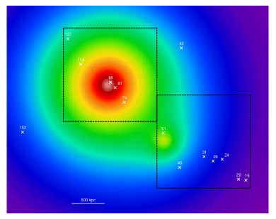
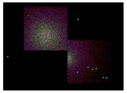
Figure 10: Left: Simulated X-ray emission for the double-$\beta$ model. Crosses mark the position of the sources in the Coma cluster and in the South-West region. Black squares mark the position where the RM has been simulated. For display purposes, ”5C4. ” is omitted in the source labels. Right: Simulated RM maps using the parameters of the standard model and two boxes of 1024³ cells (see text). White and red crosses mark the position of the sources analysed in Bonafede et al. 2010 (the two white crosses label the the position of the sources that are not taken into account in this work), cyan crosses mark the position of the sources analysed in this work.

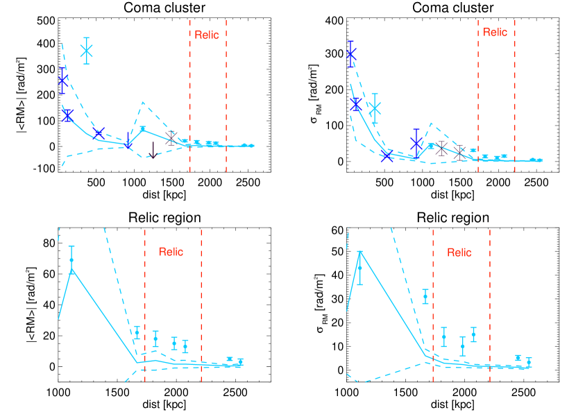
Figure 11: $\langle|\rm{RM}|\rangle$ and $\sigma_{\rm{RM}}$ derived from the ”standard” model, i.e. considering a double-beta model for the gas density and the magnetic field profile with $B_{0}=$4.7 $\mu$G and $F(n)=n^{0.5}$. Solid lines are the mean of the different random realisations, dashed lines are the 3$\sigma$ dispersion. Upper panels: crosses are the sources in the Coma cluster from Bonafede et al. (2010), dots are the sources analysed here, in the NGC 4839 group and in the relic region. Cyan symbols refer to the sources in the quadrant towards the NGC 4839 group, SW of the Coma cluster, black symbols mark the two sources that are out of the simulated box. Lower panels: zoom into the NGC4839 group and into the relic region.

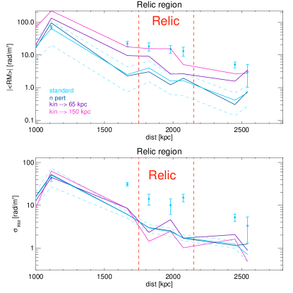
Figure 12: $\langle|\rm{RM}|\rangle$ and $\sigma_{\rm{RM}}$ trends from magnetic field models with different $k_{in}$, as shown in the plot panel. Cyan solid and dotted lines are like in Fig. 11

Table 5: Magnetic field models

Name	Gas model	$k_{\rm in}$	$k_{\rm out}$	Gaussian $dn$
single $\beta$	single $\beta$	34 kpc	2 kpc	-
standard	double $\beta$	34 kpc	2 kpc	-
n pert	double $\beta$	34 kpc	2 kpc	-
$k_{\rm in}$ 65	double $\beta$	65 kpc	2 kpc	-
$k_{\rm in}$ 150	double $\beta$	150 kpc	2 kpc	$\pm$ 10%$\times$ n
Col. 1: Reference name for the model. Col 2: model for the gas density
Col. 3 and 4: Corresponding values of $k_{in}$ and $k_{out}$ in the real space.
Col 5: Gaussian perturbation for the density model.

5.2 Alternative models for the magnetic field spectrum

We investigate here whether simple changes to the magnetic field spectrum in the NGC4839 group and in the relic region can fit the observed RM values. The parameters adopted for the individual models are listed in Table 5. The presence of a large-scale infall of gas along the South-West sectors in the Coma clusters is suggested by X-ray (Neumann et al., 2003), optical and radio (Brown & Rudnick, 2011) observations. Bulk and chaotic motions driven by large-scale motions along this direction may be responsible for the presence of magnetic field structures on scales larger compared to the innermost regions of Coma. In order to model this effect, we have simulated a magnetic field with a power spectrum similar to the one analysed in Sec. 5.1, but decreasing the value of $k_{\rm in}$. This corresponds to assigning more energy into larger eddies, as expected in the case of an ongoing merger event. In Fig. 12 the RM profiles for $k_{\rm in}$ corresponding to 65 kpc and 150 kpc are shown. An increase in the injection scale up to a length comparable to the source size has the effect of increasing the value of $\langle|\rm{RM}|\rangle$ because the biggest modes of the magnetic field are larger, and contain most of the magnetic field energy. The effect on the $\sigma_{\rm{RM}}$ depends more on the size of the source and on how many beams are sampled in the RM images. If the largest scales in the magnetic field are much larger than the size of a given radio source, the latter becomes insensitive to large-scale pattern of RM (which would lead to larger dispersion) because it can only probe smaller projected scales. The projected size of radio sources goes from $\sim$10 kpc for 5C4.16 to $\sim$ 120 kpc for 5C4.43 and the RM signal is not continuous throughout the maps. This causes the profile of $\sigma_{\rm{RM}}$ not to show a net trend with the increase of the injection scale. The fit to $\langle|\rm{RM}|\rangle$ improves as models with larger injection scales are considered, but such models provide an increasingly poor fit to $\sigma_{\rm{RM}}$.
The blue line in Fig. 12 (“n pert” model) displays the trend of $\langle|\rm{RM}|\rangle$ and $\sigma_{\rm{RM}}$ for the standard model which fits the Coma central sources, once Gaussian fluctuation of 10% in the gas density (and consequently in magnetic field) profiles are added on scales of $\sim$ 100 kpc. These perturbations are consistent with the typical amount of brightness fluctuations observed in the centre of Coma (Churazov et al., 2012), and with those measured by hydrodynamical simulations at such large radii (Vazza et al., 2013). Adding gas perturbations investigates the possible role of enhanced gas clumping along the South-West sector, which would simultaneously affect the density and the magnetic (through $\propto n^{0.5}$ scaling) structure. However, the deviations from the standard profile are small and do not change significantly the RM statistics.
Hence, we can conclude that neither a change in the power spectrum nor the standard spectrum with the addition of Gaussian random fluctuations of the order of 10% are able to reproduce simultaneously the observed trends of $\sigma_{\rm{RM}}$ and $\langle|\rm{RM}|\rangle$ in the relic region.

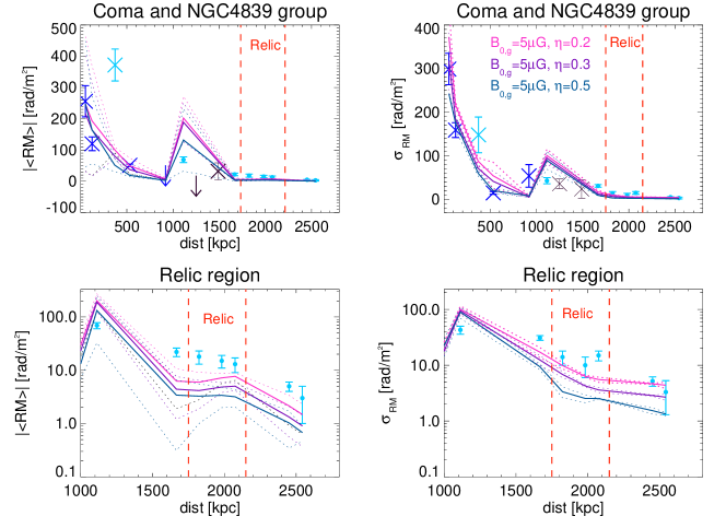
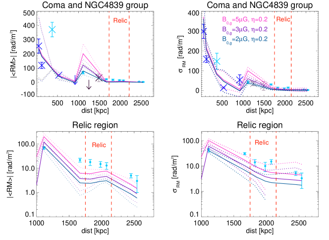
Figure 13: $\langle|\rm{RM}|\rangle$ and $\sigma_{\rm{RM}}$ trend versus the projected distance from the cluster centre. Crosses are the points from Bonafede et al. (2010), dots are the new points from this paper. Blue symbols mark the sources in the Coma cluster, cyan symbols mark those SW from the cluster centre, in the direction of the Coma relic. Black crosses mark the position of the sources that are outside the simulated box. Red vertical lines indicate the approximate location of the Coma relic. Continuous lines display the average among the different realisations, dotted lines display the dispersion. Top panels: $\langle|\rm{RM}|\rangle$ and $\sigma_{\rm{RM}}$ trends are displayed for three representative models obtained by changing the value of $\eta_{g}$, as written in upper right panel. Bottom panels: $\langle|\rm{RM}|\rangle$ and $\sigma_{\rm{RM}}$ trends are displayed for different values of $B_{0,g}$ and $\eta_{g}=0.2$, as written in the mid-right panel.

5.3 The magnetic field in the NGC4839 group

The group NGC4839 can be modelled as an independent group falling into the Coma cluster. In Sec. 5.1 we have shown that the scaling $B(r)\propto n^{0.5}$ inferred from Coma gives a reasonable description of the RM values at the centre of the group, but does not reproduce within 3$\sigma$ the values of the other sources analysed in this work. Although the $\beta$-model used for the group does not provide an accurate description of the gas distribution, we attempt to fit the RM values for the sources in the SW sector by assuming an independent magnetic field model for the NGC4839 group. We have assumed the following scalings for the magnetic field in the group:

$$B_{\rm group}(r)=\hat{B}_{g}\left(\frac{n_{g}(r)}{n_{0}}\right)^{\eta_{g}}$$ (8)

and for the Coma cluster:

$$B_{\rm Coma}(r)=\hat{B}\left(\frac{n_{c}(r)}{n_{0}}\right)^{\eta}$$ (9)

and the same values of $k_{\rm in}$ and $k_{\rm out}$ as found in Bonafede et al. (2010). We have realised independent grids of 3D magnetic fields for the two systems, and added them together in the regions of interest. The fact that $\nabla\cdot{\bf B}=0$ by construction in both grids allows us to perform this operation preserving the zero-divergence condition with the same accuracy. The centre of the group along the line of sight is placed on the same plane as the Coma cluster’s centre. We have then obtained mock RM images by integrating numerically the equation

$$RM=\int{(B_{\rm{Coma},z}\times n_{c}+B_{\rm{group},z}\times n_{g})dl}$$ (10)

changing the values of $B_{0,g}$ from 2 to 10 $\mu$G and $\eta_{g}$ from 0.2 to 0.5. Since flat magnetic field profiles for the group could affect also the RM values of the Coma cluster sources, we have compared mock and real RM images for all the sources in the field. In Fig. 13 we show the results for the most representative cases among those analysed. In the top panels, three models with different $\eta_{g}$ are shown. We note that as the profile flattens (i.e. $\eta_{g}$ decreases), the RM values at the centre of the group increase, as expected since the RM is an integrated quantity along the line of sight, and it is sensitive to the magnetic field in the outer parts of the group. Hence, although using flatter profiles $\sigma_{\rm{RM}}$ and $\langle|\rm RM|\rangle$ become closer to the observed values in the relic region, they provide a worse fit in the centre of the group. Even a flat magnetic field profile ($\eta_{g}=0.2$) is not able to reproduce the observed values of $\sigma_{\rm{RM}}$ and $\langle|\rm RM|\rangle$ irrespective of $B_{0,g}$. As shown in the bottom panels of Fig. 13, values of $B_{0,g}$ of the order of 2 $\mu$G are required for the centre of the group, while higher values would be needed in the relic region and beyond.
We conclude that, in the double $\beta$-model approximation, there is no obvious combination of values for $B_{0,g}$ and $\eta_{g}$ which is able to reproduce the observed RMs in the SW sector of the Coma cluster. Even flat profiles with $\eta_{g}=$0.2 fail in describing the trends of $\sigma_{\rm{RM}}$ and $\langle|\rm RM|\rangle$ in the SW region.

6 Discussion

We tried to model the 3D structure of the magnetic field in the Coma cluster and along the relic sector by simulating different configurations of ${\bf B}$, similar to what has been already done in the literature (e.g. Murgia et al., 2004; Bonafede et al., 2010; Vacca et al., 2012).
The extrapolation of the magnetic field model that successfully reproduces the trend of RM in the Coma cluster (Bonafede et al., 2010) does not reproduce the trend of RM along the SW sector. The values of $\langle|\rm RM|\rangle$ and $\sigma_{\rm RM}$ are nearly one order of magnitude lower than the observed values.
Several independent works have found large-scale accretion patterns in the SW region of the Coma cluster, using X-ray observations (Neumann et al., 2003; Ogrean & Brüggen, 2012; Akamatsu et al., 2013; Simionescu et al., 2013, see however Bowyer et al. 2004 for a different interpretation ) , optical observations (Colless & Dunn, 1996; Neumann et al., 2001; Brown & Rudnick, 2011), and radio observations (e. g. Brown & Rudnick, 2011). Therefore, a significant departure from the simple $\beta$-model profile along this direction is very likely.
We tested this scenario simulating a double-$\beta$-model, which considers a second spherical gas concentration coincident with the group NGC4839. We assumed for the group a core radius and a central density which are the rescaled version of the Coma cluster for a system with one tenth of the mass, as indicated by Neumann et al. (2001). We have produced 3D magnetic field simulations for this double $\beta$-model, normalising the mean magnetic field at 4.7 $\mu$G within the Coma core radius, and scaling the magnetic field profile with the square-root of the gas density throughout the whole simulated volume. This choice gives a mean magnetic field within the core radius of the group of 3.6 $\mu$G. We find that at 99% confidence level, the values of $\langle|\rm{RM}|\rangle$ and $\sigma_{\rm RM}$ at the location of 5C4.51, the brightest galaxy of the group, can be explained by the double $\beta$-model. However, along a sector of $\sim 1\rm Mpc$ further to the SW, the observed values of the Faraday Rotation are still larger than the simulated double $\beta$-model by a factor $\sim 6$. Basic modifications to the 3D model that we have tried (e.g. by imposing different spectra, or adding some amount of gas clumping to the simulated gas model) are unable to simultaneously reproduce $\langle|\rm{RM}|\rangle$ and $\sigma_{\rm RM}$ for all the sources. We have also attempted to reproduce the RM values in the group by fitting independently a magnetic field model for the group and then adding the contribution of the Coma cluster. Even very flat magnetic field profiles ($\eta_{g}=$0.2) are unable to reproduce the trends of $\langle|\rm RM|\rangle$ and $\sigma_{\rm RM}$ along the entire SW sector out to the relic and beyond. We note that magnetic field profiles flatter than $\eta=0.2$ would be in disagreement with previous works (e.g. Govoni et al., 2006; Guidetti et al., 2008; Bonafede et al., 2010) and also with cosmological MHD simulations (e.g. Donnert et al., 2010; Skillman et al., 2013; Dolag et al., 2008, and ref. therein).
Hence, we conclude that the RM data along the SW sector of the Coma cluster require additional amplification of the magnetic field.

6.1 Limits to the magnetic field and gas density in the relic region

In order to understand how the gas and the magnetic field contribute to the RM enhancement, it would be necessary to derive independent estimates or limits for the two, separately. Although it is not possible to derive limits for the magnetic field, recent Suzaku X-ray observations provide useful constraints on the gas density at the position of the relic (Akamatsu et al., 2013; Simionescu et al., 2013). From the brightness profiles present in the two recent papers, we have computed the corresponding density profiles assuming a constant temperature. The two profiles are shown in Fig. 14. The small differences between the two are due to the different regions used for spectral analysis, and to slightly different de-projection assumptions used in the two works. Although the double $\beta$-model that we are using is only a first-order approximation for the real gas density distribution in the system, the density profile at the position of the relic is compatible with the real gas density within a$\sim 50$ percent (see Fig.14), while it is higher by a factor $\sim$ 5 inside the core radius of the group. This suggests that the larger observed values of Faraday Rotation along the SW sector cannot be explained by a medium much denser than what assumed here, unless it is too cold ($T<10^{7}\rm K$) to emit in X-rays. However, the overall good agreement between the outer gas density profiles obtained through X-ray and SZ observations (Planck Collaboration et al., 2012; Fusco-Femiano et al., 2013) makes this scenario unlikely.
A uniform boost in the magnetic field by a factor $\sim 6$ would reconcile with the data in a rather simple way, yielding an average level of magnetic field of $\sim 3-4\;\mu\rm G$ at the location of the relic. This value would be about 3 times higher than the radio equipartition values (Thierbach et al., 2003), and compatible with the lower limits provided by the Inverse Compton analysis (e.g. Feretti & Neumann, 2006). The boost factor can be reduced to $\sim 3$ if the gas density suggested by the most recent X-ray observations is used, yielding a value of $\sim 1.5-2\;\mu\rm G$ at the location of the relic. Magnetic field with strength of the order of few $\mu$G in radio relics are found by cosmological simulations (Skillman et al., 2008) and using radio equipartition estimates (e.g. Bonafede et al., 2009; Giovannini et al., 2010). However, our data suggest that the required magnetic boost is not limited to the relic region - which is $\sim$ 400 kpc wide- but extends up to a distance of $\sim 1.5\;\rm Mpc$ from the group centre, although the large uncertainties in the region beyond the relic do not allow significant constraints on the gas density (see Fig. 14).

6.2 Implications on dynamics

The derived values of the magnetic field along the SW sector have no important impact on the cluster dynamics. The plasma beta, $\beta_{\rm pl}$, can be estimated as $\beta_{\rm pl}\approx 2c^{2}_{\rm s}/v^{2}_{\rm A}$, where $c_{\rm s}$ is the gas sound speed and $v_{\rm A}$ is the Alfvén speed. The presence of the X-ray emitting gas yields $\beta_{\rm pl}\approx 10-100$, and therefore the magnetic pressure is still dynamically irrelevant.
A rather natural way of producing such large-scale magnetic fields is a cosmic filaments along the SW direction, a possibility that has been already suggested elsewhere (Finoguenov et al., 2003; Brown & Rudnick, 2011), and that emerges from MHD cosmological simulations as well (Brüggen et al., 2005; Dolag et al., 2005a). However, the observed values of $\sigma_{\rm RM}$ indicate a broad spectrum of fluctuations, in the range 2 - 50 kpc at least, which are not expected in cosmic filaments. Instead, cosmological simulations indicate that the topology of the magnetic field in filaments is ordered and uniform, because the eddy turnover-time of turbulent motions is larger than the filaments’ age, and turbulence is not fully developed (e.g. Ryu et al., 2008). The observed dispersion in the RM for the sources observed through the relic indicates that turbulent motions are present in the relic region.
If a shock is present across the Coma relic, as suggested by recent X-ray observations (Ogrean & Brüggen, 2012; Akamatsu et al., 2013), some magnetic field amplification is expected. It was recently shown by Iapichino & Brüggen (2012) that most of the amplification is due to the compression of the ICM plasma, while turbulence should play a minor role, although under certain circumstances vorticity generated by compressive and baroclinic effects across the shock discontinuity can lead to a sufficient amplification of the magnetic field. We note that the observed RMs require an enhancement of the $B_{//}\times n$ quantity not only in the region of the relic, but over the full SW sector ($\sim$ 1.5 Mpc). In agreement with this result is the presence of a weak radio emission connecting the halo, the relic, and the radio galaxy 5C4.20. Indeed, the radio halo and the radio relic of the Coma cluster are connected through a low-brightness radio bridge (Venturi et al., 1989; Giovannini et al., 1993; Brown & Rudnick, 2011), and on the Western side of the relic a similar low-brightness radio bridge connects the relic with the radiogalaxy 5C4.20 (Giovannini et al., 1991). In addition, single dish observations of the Coma cluster have shown a large amount of diffuse synchrotron emission in the SW region of the cluster, extending to at least $\sim$ 2.4 Mpc west of the centre of the Coma cluster’s radio halo (Kronberg et al., 2007; Brown & Rudnick, 2011). Hence, the observed presence of large-scale relativistic electrons and magnetic fields, probed by radio observations, the elongated X-ray and SZ morpohologies (Neumann et al., 2001; Finoguenov et al., 2003; Planck Collaboration et al., 2012), and the hint of a weak shock, $M\sim 2$, at the relic location (Ogrean & Brüggen, 2012; Akamatsu et al., 2013) suggest that a more inhomogeneous large-scale accretion event is taking place. In this framework, the virialisation of the kinetic energy would not be completed yet, yielding to a magnetic field and gas density amplification. Although in this work we do not attempt to model further the dynamics of the ICM along the SW direction, the agreement between the density profile used here and the one derived by recent Suzaku observations indicate that the limits on the magnetic field at the position of the relic are robust.
A more sophisticated analysis can be done by using more realistic distributions for the ICM gas in the SW sector, and relaxing the assumption of an isotropic magnetic field. A possibility to explain the observed RM trends would be a large-scale component of the magnetic field, aligned with the filament which is accreting matter into Coma, plus smaller scale components that would give the observed RM dispersion. Such a configuration, opportunely projected along the line of sight, could in principle produce the observed $\sigma_{\rm RM}$ and $\langle|\rm RM|\rangle$ trends. We will tackle this issue in a forthcoming work.

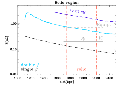
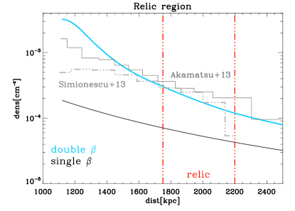
Figure 14: Top: Magnetic field profiles in the group and relic region. The black dashed-double dotted line displays the profile obtained by Bonafede et al (2010) for the Coma sources, the cyan line displays the profiles from the standard model, assuming a double-$\beta$ model for the gas density, $B_{0}=4.7\;\mu$G and $F(n)=n^{0.5}$. The blu dashed line displays the magnetic field needed to fit the RM data in the relic region and beyond. Overplotted are the lower limits from the Inverse Compton (Feretti & Neumann, 2006), and the estimate from Equipartition (Thierbach et al., 2003). Bottom: Gas density profile in the group and relic region. The black line displays the single $\beta$-model for Coma, the cyan line displays the double $\beta$-model for Coma and NGC4839 group. Grey lines display the profile derived by Suzaku observations.

7 Conclusions

In this work we have presented new RM data for seven sources located across the Coma relic. The trends of $\sigma_{\rm RM}$ and $\langle|\rm RM|\rangle$ have been analysed together with the data presented in Bonafede et al. (2010), to probe the magnetic field properties in the outskirts of the cluster, where the radio relic is located. We have presented a new tool to interpret the RM data by comparing mock and real RM observations. The main results can be summarised as follows:

• Both $\sigma_{\rm RM}$ and $\langle|\rm RM|\rangle$ decrease going from the centre of the NGC4839 group towards the outskirts of the cluster, indicating that both the gas density and the magnetic field profile decrease radially. No evident jump is found at the position of the relic.
  

• The observed values of $\sigma_{\rm RM}$ indicates the presence of a magnetic field which fluctuates over a range of spatial scales, possibly indicating turbulent motions in the SW region of the cluster, across the relic and beyond.
  

• Both $\sigma_{\rm RM}$ and $\langle|\rm RM|\rangle$ are higher than predicted by simply extrapolating the magnetic field and the gas density profiles which, instead, give the best fit for the RMs in the Coma cluster.
  

• When a double $\beta$-model is used to describe the gas density profile in the system Coma - NGC4839 group, the best fit values found for the magnetic field in the Coma cluster, e.g. $B_{0}=4.7\,\mu$G and $F(n)\propto 0.5$ (Bonafede et al., 2010) reproduce the values of $\sigma_{RM}$ and $\langle|\rm RM|\rangle$ only for the brightest source of the group: 5C4.51 (NGC4839). This magnetic field model gives an average magnetic field of 3.6 $\mu$G within the group core radius. The trends of $\sigma_{\rm RM}$ and $\langle|\rm RM|\rangle$ for the remaining six sources in the SW sector are underestimated by a factor 6 - 8. By comparing these data with recent gas density estimates from Suzaku (Akamatsu et al., 2013; Simionescu et al., 2013) we have derived that a boost of the magnetic field by a factor $\sim$ 3 is required.
  

• The magnetic field amplification does not appear to be limited to the relic region, but it must occur throughout the whole SW sector ($\sim 1.5$ Mpc).
  

• There is no simple combination of $\beta$-models for Coma and the NGC4839 group that can reproduce the observed trends of $\sigma_{\rm RM}$ and $\langle|\rm RM|\rangle$ at the same time. Similarly, neither a change in the magnetic field power spectrum in the SW sector, neither adding gaussian perturbation to the gas density and to the magnetic field can help is reconciling observed and simulated values.
  

• The analysis of these data together with the available results from X-ray (Neumann et al., 2003; Ogrean & Brüggen, 2012; Akamatsu et al., 2013; Simionescu et al., 2013), optical (Colless & Dunn, 1996; Neumann et al., 2001; Brown & Rudnick, 2011), SZ (Planck Collaboration et al., 2012), and radio (Giovannini et al., 1991; Kronberg et al., 2007; Brown & Rudnick, 2011) observations indicate that the most plausible scenario is the one in which a large-scale accretion event, followed by a yet incomplete virialisation of kinetic energy, is taking place in the SW region of the Coma cluster, yielding to a significant magnetic field amplification.
  

• In order to reconcile mock and observed RM trends in the SW region, the magnetic field must have been amplified by a factor $\sim$3. In this case, the magnetic field across the relic region should be then $\sim$ 2 $\mu$G, which is consistent with IC upper limits.
  

Acknowledgments The authors thank K.Dolag for fruitful discussions and for the use of Pacerman. AB, MB, and FV acknowledge support by the research group FOR 1254 funded by the Deutsche Forschungsgemeinschaft: “Magnetization of interstellar and intergalactic media: the prospect of low frequency radio observations”. This research has made use of the NASA/IPAC Extragalactic Data Base (NED) which is operated by the JPL, California institute of Technology, under contract with the National Aeronautics and Space Administration.

References

- Akamatsu et al. (2013) Akamatsu, H., Inoue, S., Sato, T., et al. 2013, ArXiv e-prints
- Akamatsu & Kawahara (2013) Akamatsu, H. & Kawahara, H. 2013, PASJ, 65, 16
- Baars et al. (1977) Baars, J. W. M., Genzel, R., Pauliny-Toth, I. I. K., & Witzel, A. 1977, A&A, 61, 99
- Becker et al. (1995) Becker, R. H., White, R. L., & Helfand, D. J. 1995, ApJ, 450, 559
- Bonafede et al. (2011b) Bonafede, A., Dolag, K., Stasyszyn, F., Murante, G., & Borgani, S. 2011b, MNRAS, 418, 2234
- Bonafede et al. (2010) Bonafede, A., Feretti, L., Murgia, M., et al. 2010, A&A, 513, A30
- Bonafede et al. (2009) Bonafede, A., Giovannini, G., Feretti, L., Govoni, F., & Murgia, M. 2009, A&A, 494, 429
- Bonafede et al. (2011a) Bonafede, A., Govoni, F., Feretti, L., et al. 2011a, A&A, 530, A24+
- Bowyer et al. (2004) Bowyer, S., Korpela, E. J., Lampton, M., & Jones, T. W. 2004, ApJ, 605, 168
- Briel et al. (1992) Briel, U. G., Henry, J. P., & Boehringer, H. 1992, A&A, 259, L31
- Brown & Rudnick (2011) Brown, S. & Rudnick, L. 2011, MNRAS, 412, 2
- Brüggen et al. (2011) Brüggen, M., Bykov, A., Ryu, D., & Röttgering, H. 2011, Space Science Reviews, 138
- Brüggen et al. (2005) Brüggen, M., Ruszkowski, M., Simionescu, A., Hoeft, M., & Dalla Vecchia, C. 2005, ApJ, 631, L21
- Cavaliere & Fusco-Femiano (1976) Cavaliere, A. & Fusco-Femiano, R. 1976, A&A, 49, 137
- Chen et al. (2008) Chen, C. M. H., Harris, D. E., Harrison, F. A., & Mao, P. H. 2008, MNRAS, 383, 1259
- Churazov et al. (2012) Churazov, E., Vikhlinin, A., Zhuravleva, I., et al. 2012, MNRAS, 421, 1123
- Clarke (2004) Clarke, T. E. 2004, Journal of Korean Astronomical Society, 37, 337
- Colless & Dunn (1996) Colless, M. & Dunn, A. M. 1996, ApJ, 458, 435
- Condon et al. (1998) Condon, J. J., Cotton, W. D., Greisen, E. W., et al. 1998, AJ, 115, 1693
- Dolag et al. (1999) Dolag, K., Bartelmann, M., & Lesch, H. 1999, A&A, 348, 351
- Dolag et al. (2008) Dolag, K., Bykov, A. M., & Diaferio, A. 2008, Space Science Reviews, 134, 311
- Dolag et al. (2005a) Dolag, K., Grasso, D., Springel, V., & Tkachev, I. 2005a, Journal of Cosmology and Astro-Particle Physics, 1, 9
- Dolag & Stasyszyn (2009) Dolag, K. & Stasyszyn, F. 2009, MNRAS, 398, 1678
- Dolag et al. (2005b) Dolag, K., Vogt, C., & Enßlin, T. A. 2005b, MNRAS, 358, 726
- Donnert et al. (2010) Donnert, J., Dolag, K., Brunetti, G., Cassano, R., & Bonafede, A. 2010, MNRAS, 401, 47
- Ensslin et al. (1998) Ensslin, T. A., Biermann, P. L., Klein, U., & Kohle, S. 1998, A&A, 332, 395
- Ensslin et al. (2003) Ensslin, T. A., Vogt, C., Clarke, T. E., & Taylor, G. B. 2003, ApJ, 597, 870
- Feretti et al. (1999) Feretti, L., Dallacasa, D., Govoni, F., et al. 1999, A&A, 344, 472
- Feretti et al. (2012) Feretti, L., Giovannini, G., Govoni, F., & Murgia, M. 2012, A&AR
- Feretti & Neumann (2006) Feretti, L. & Neumann, D. M. 2006, A&A, 450, L21
- Finoguenov et al. (2003) Finoguenov, A., Briel, U. G., & Henry, J. P. 2003, A&A, 410, 777
- Finoguenov et al. (2010) Finoguenov, A., Sarazin, C. L., Nakazawa, K., Wik, D. R., & Clarke, T. E. 2010, ApJ, 715, 1143
- Fusco-Femiano et al. (2013) Fusco-Femiano, R., Lapi, A., & Cavaliere, A. 2013, ApJ, 763, L3
- Giovannini et al. (2010) Giovannini, G., Bonafede, A., Feretti, L., Govoni, F., & Murgia, M. 2010, A&A, 511, L5
- Giovannini et al. (1991) Giovannini, G., Feretti, L., & Stanghellini, C. 1991, A&A, 252, 528
- Giovannini et al. (1993) Giovannini, G., Feretti, L., Venturi, T., Kim, K.-T., & Kronberg, P. P. 1993, ApJ, 406, 399
- Govoni et al. (2010) Govoni, F., Dolag, K., Murgia, M., et al. 2010, A&A, 522, A105+
- Govoni et al. (2006) Govoni, F., Murgia, M., Feretti, L., et al. 2006, A&A, 460, 425
- Guidetti et al. (2012) Guidetti, D., Laing, R. A., Croston, J. H., Bridle, A. H., & Parma, P. 2012, MNRAS, 423, 1335
- Guidetti et al. (2008) Guidetti, D., Murgia, M., Govoni, F., et al. 2008, A&A, 483, 699
- Hoeft & Brüggen (2007) Hoeft, M. & Brüggen, M. 2007, MNRAS, 375, 77
- Iapichino & Brüggen (2012) Iapichino, L. & Brüggen, M. 2012, MNRAS, 423, 2781
- Johnston-Hollitt et al. (2004) Johnston-Hollitt, M., Hollitt, C. P., & Ekers, R. D. 2004, in The Magnetized Interstellar Medium, ed. B. Uyaniker, W. Reich, & R. Wielebinski, 13–18
- Kang & Ryu (2011) Kang, H. & Ryu, D. 2011, ApJ, 734, 18
- Kang et al. (2012) Kang, H., Ryu, D., & Jones, T. W. 2012, ArXiv e-prints
- Kronberg et al. (2007) Kronberg, P. P., Kothes, R., Salter, C. J., & Perillat, P. 2007, ApJ, 659, 267
- Macario et al. (2011) Macario, G., Markevitch, M., Giacintucci, S., et al. 2011, ApJ, 728, 82
- Markevitch et al. (2002) Markevitch, M., Gonzalez, A. H., David, L., et al. 2002, ApJ, 567, L27
- Markevitch et al. (2005) Markevitch, M., Govoni, F., Brunetti, G., & Jerius, D. 2005, ApJ, 627, 733
- McMahon et al. (2002) McMahon, R. G., White, R. L., Helfand, D. J., & Becker, R. H. 2002, ApJS, 143, 1
- Murgia et al. (2004) Murgia, M., Govoni, F., Feretti, L., et al. 2004, A&A, 424, 429
- Neumann et al. (2001) Neumann, D. M., Arnaud, M., Gastaud, R., et al. 2001, A&A, 365, L74
- Neumann et al. (2003) Neumann, D. M., Lumb, D. H., Pratt, G. W., & Briel, U. G. 2003, A&A, 400, 811
- Ogrean & Brüggen (2012) Ogrean, G. A. & Brüggen, M. 2012, ArXiv e-prints
- Ogrean et al. (2013) Ogrean, G. A., Brüggen, M., Röttgering, H., et al. 2013, MNRAS, 429, 2617
- O’Sullivan et al. (2013) O’Sullivan, S. P., Feain, I. J., McClure-Griffiths, N. M., et al. 2013, ArXiv e-prints
- Planck Collaboration et al. (2012) Planck Collaboration, Ade, P. A. R., Aghanim, N., et al. 2012, ArXiv e-prints
- Russell et al. (2011) Russell, H. R., van Weeren, R. J., Edge, A. C., et al. 2011, MNRAS, 417, L1
- Ruszkowski et al. (2011) Ruszkowski, M., Lee, D., Brüggen, M., Parrish, I., & Oh, S. P. 2011, ApJ, 740, 81
- Ryu et al. (2008) Ryu, D., Kang, H., Cho, J., & Das, S. 2008, Science, 320, 909
- Ryu et al. (2003) Ryu, D., Kang, H., Hallman, E., & Jones, T. W. 2003, ApJ, 593, 599
- Simard-Normandin et al. (1981) Simard-Normandin, M., Kronberg, P. P., & Button, S. 1981, ApJS, 45, 97
- Simionescu et al. (2013) Simionescu, A., Werner, N., Urban, O., et al. 2013, ArXiv e-prints
- Skillman et al. (2008) Skillman, S. W., O’Shea, B. W., Hallman, E. J., Burns, J. O., & Norman, M. L. 2008, ApJ, 689, 1063
- Skillman et al. (2012) Skillman, S. W., Xu, H., Hallman, E. J., et al. 2012, ArXiv e-prints
- Skillman et al. (2013) Skillman, S. W., Xu, H., Hallman, E. J., et al. 2013, ApJ, 765, 21
- Smith et al. (2000) Smith, R. J., Lucey, J. R., Hudson, M. J., Schlegel, D. J., & Davies, R. L. 2000, MNRAS, 313, 469
- Taylor et al. (2002) Taylor, G. B., Fabian, A. C., & Allen, S. W. 2002, MNRAS, 334, 769
- Thierbach et al. (2003) Thierbach, M., Klein, U., & Wielebinski, R. 2003, A&A, 397, 53
- Vacca et al. (2012) Vacca, V., Murgia, M., Govoni, F., et al. 2012, A&A, 540, A38
- van Weeren et al. (2010) van Weeren, R. J., Röttgering, H. J. A., Brüggen, M., & Hoeft, M. 2010, Science, 330, 347
- Vazza et al. (2010) Vazza, F., Brunetti, G., Gheller, C., & Brunino, R. 2010, New Astr, 15, 695
- Vazza et al. (2011) Vazza, F., Dolag, K., Ryu, D., et al. 2011, MNRAS, 418, 960
- Vazza et al. (2013) Vazza, F., Eckert, D., Simionescu, A., Brüggen, M., & Ettori, S. 2013, MNRAS, 429, 799
- Venturi et al. (1989) Venturi, T., Feretti, L., & Giovannini, G. 1989, A&A, 213, 49
- Venturi et al. (1990) Venturi, T., Giovannini, G., & Feretti, L. 1990, AJ, 99, 1381