Theory for entanglement of electrons dressed with circularly polarized light in Graphene and three-dimensional Topological insulators

Abstract

We have formulated a theory for investigating the conditions which are required to achieve entangled states of electrons on graphene and three-dimensional (3D) topological insulators (TIs). We consider the quantum entanglement of spins by calculating the exchange energy. A gap is opened up at the Fermi level between the valence and conduction bands in the absence of doping when graphene as well as 3D TIs are irradiated with circularly-polarized light. This energy band gap is dependent on the intensity and frequency of the applied electromagnetic field. The electron-photon coupling also gives rise to a unique energy dispersion of the dressed states which is different from either graphene or the conventional two-dimensional electron gas (2DEG). In our calculations, we obtained the dynamical polarization function for imaginary frequencies which is then employed to determine the exchange energy. The polarization function is obtained with the use of both the energy eigenstates and the overlap of pseudo-spin wave functions. We have concluded that while doping has a significant influence on the exchange energy and consequently on the entanglement, the gap of the energy dispersions affects the exchange slightly, which could be used as a good technique to tune and control entanglement for quantum information purposes.

1 INTRODUCTION

Topological insulators (TIs), being a novel quantum state of matter, were first predicted theoretically in 2006 [1] and then observed in experiment. [2] The main feature defining TIS is the existence of an insulating gap in the bulk and topologically protected conducting states localized on its boundaries [3, 4] . Conventional classification of TIs follows from their geometry. Historically, two-dimensional (2D) TIs, which are also referred to as quantum spin Hall (QSH) insulators as well as their predecessors quantum Hall states, represented the first state, which did not fit into Landau-Ginzburg description of a state of matter by the symmetry and order parameter. The first experimental realization of 2D TIs was given in HgTe/CdTe quantum wells, where the non-trivial topological state can be observed if the thickness of the sample is more than a certain critical value ($\backsimeq 6.1\,nm$ for HgTe).

From a theoretical point of view, 3D TIs were first predicted and later confirmed in Bi₂Te₃ and Sb₂Te₃. Similar to the case of 2D TIs, they could be characterized by a large insulating gap in the bulk and the spin-polarized surface states are like graphene, protected from backscattering. The latter property results from the fact that in the linear approximation the above mentioned surface states are described by a Dirac cone. The electrons in 3D TIs are also represented by a helical liquid, meaning that the electron spins are perpendicular to the momentum. Such states cannot appear in normal 2D system with time-reversal symmetry. Consequently, they are also referred to as holographic.

It has been demonstrated experimentally[5] that exposing the surface of a 3D TI to circularly-polarized light induces photo-currents. The light polarization could be used to produce and control photo currents. These currents represent non-equilibrium properties and are unique for 3D TIs. These currents may also result in an opportunity to measure fundamental physical quantities such as the Berry phase. A similar current arising from topological states could appear as a result of the interaction of 3D TI surface Dirac electrons with linearly-polarized light.

The states with an opened energy gap along with their collective properties are the central concern of this paper. A geometrical gap is observed in the case of a finite sized sample in the $x-$direction, say[6, 7]. The advantage of inducing a gap with circularly polarized light is it being tunable, i.e., the gap could be controlled by changing the intensity of the radiation. The effects of the gap opening were considered classically for both graphene [8, 9] and TIs.[10, 11] Additionally, there have been a number of studies using laser radiation on single layer[12] and bilayer[13] graphene as well as graphene nanoribbons[14, 15] reporting the gap opening as the result of electron-photon interaction. From these considerations, it seems that TIs and gapped graphene may have potential applications in devices where spin plays a role.

The rest of the paper is organized as follows. In Sec. 2, we present a brief description as well as derive the electron-photon dressed states in topological insulators, which we previously obtained [16] but include for completeness and to introduce our notation. After that, we calculate the dynamical polarization function for both real and imaginary frequencies. Only the latter may be employed to evaluate the electron exchange energy. We compare the response function for interacting electrons in the random phase approximation (RPA) at frequencies on the imaginary axis with that obtained for frequencies with a small imaginary part since they are used in calculating the correlation energy and collective plasma excitations, respectively. Our results which were obtained numerically are in agreement with those obtained analytically for plasmons in Dirac-cone graphene[17, 18], gapped graphene  [19] and TIs [20], thereby giving credibility to our calculations for the exchange energy. It appears that the effect due to the quadratic term $\backsim\mathcal{D}k^{2}$ correction to the linear energy dispersion in wave vector $k$ has little influence on the overlap structure factor. This is also demonstrated in Sec. 3. The difference in the single electron energy dispersions is not negligible far from the Dirac point. Consequently, this does not affect the electron polarization function in the long wave limit. Finally, Sec. 4 is devoted to our numerical calculations of the electron exchange energy, which has been used as a measure of the electron entanglement in quantum dots[21, 22] and in the troughs formed by surface acoustic waves.[23] We have demonstrated that the chemical potential (doping) $\mu$ has a significant effect on the exchange energy. On the other hand, the electron energy gap only affects the exchange by a few percent, thus providing a novel technique for sensitively tuning the electron entanglement, which may receive significant applications in the field of quantum computing by isolating pairs of dressed Dirac electrons in quantum dots. We provide some concluding remarks in Sec.  5.

2 Electron-photon dressed states in graphene and topological insulators

In this section, we provide a rigorous analytic derivation and discussion of dressed states on the surface of a 3D TI. As we show below, the electron interaction with circularly polarized photons is the only case for which a complete analytic solution may be obtained. Apparently, due to the specific wave number $k-$dependence of the Hamiltonian, relatively similar solutions may be obtained for both graphene and 3D TIs [16] .

Analysis of dressed stated in graphene  [24, 25] showed that electrons in graphene may acquire a gap due to the interaction with circularly- polarized photons. The corresponding wave function is no longer chiral and this leads to specific tunneling and transport properties [26] .

The Hamiltonian describing surface states (at $z=0$) of a 3D TI to order of ${\cal O}(k^{2})$ is given by  [27]

$$\mathcal{H}^{surf}_{3D}=\mathcal{D}k^{2}+\mathcal{A}\sigma\cdot{k}=\left({\begin{array}[]{cc}\mathcal{D}k^{2}&\mathcal{A}k_{-}\\ \mathcal{A}k_{+}&\mathcal{D}k^{2}\end{array}}\right)\ ,$$ (1)

where ${\bf k}=(k_{x},\,k_{y})$ is the in-plane surface wave vector and $k_{\pm}=k_{x}\pm ik_{y}$. Here, we take into consideration the diagonal mass terms $\backsim\mathcal{D}k^{2}$ in conjunction with the standard Dirac cone terms $\mathcal{A}k_{\pm}$.The energy dispersion associated with this Hamiltonian is given by $\varepsilon^{\rm surf}_{3D}=\mathcal{D}k^{2}+\beta\mathcal{A}k$ with $\beta=\pm 1$.

Let us now consider electron-photon interaction on the surface of a 3D TI. We first assume that the surface of the 3D TI is irradiated by circularly polarized light with its quantized vector potential given by

$$\hat{\mathbf{A}}=\mathcal{F}_{0}\left(\mathbf{e}_{+}\,\hat{a}+\mathbf{e}_{-}\,\hat{a}^{{\dagger}}\right)\ ,$$ (2)

where the left and right circular polarization unit vectors are denoted by $\mathbf{e}_{\pm}=(\mathbf{e}_{x}\pm i\,\mathbf{e}_{y})/\sqrt{2}$,and $\mathbf{e}_{x}$ ($\mathbf{e}_{y}$) is the unit vector in the $x$ ($y$) direction. The amplitude of the circularly polarized light is related to the photon angular frequency $\omega_{0}$ by $\mathcal{F}_{0}\sim\sqrt{1/\omega_{0}}$. Here, we consider a weak field (energy $\sim\mathcal{F}^{2}_{0}$) compared to the photon energy $\hbar\omega_{0}$. Additionally, the total number $N_{0}$ of photons is fixed for the optical mode represented by Eq. (2), corresponding to the case with focused light incident on a portion of an optical lattice modeled by Floquet theory [8].

We now turn to the case when the surface of the 3D TI is irradiated by circularly polarized light with vector potential

$$\hat{\mathbf{A}}={\cal F}_{0}\left(\texttt{\bf e}_{+}\hat{a}+\texttt{\bf e}_{-}\hat{a}^{{\dagger}}\right)\ ,$$ (3)

where $\texttt{\bf e}_{\pm}=(\texttt{\bf e}_{x}\pm i\texttt{\bf e}_{y})/\sqrt{2}$, $\texttt{\bf e}_{x}$ and $\texttt{\bf e}_{y}$ are unit vectors in the $x$ and $y$ direction, respectively. Consequently, the in-plane components of the vector potential may be expressed as

$$\hat{A}_{x}=\frac{{\cal F}_{0}}{\sqrt{2}}(\hat{a}+\hat{a}^{{\dagger}})\ ,\hskip 18.06749pt\hat{A}_{y}=i\frac{{\cal F}_{0}}{\sqrt{2}}(\hat{a}-\hat{a}^{{\dagger}})\ .$$ (4)

In order to include electron-photon coupling, we make the following substitution for electron wave vector

$$k_{x}\longrightarrow k_{x}+\frac{e\hat{A}_{x}}{\hbar}=k_{x}+\frac{e{\cal F}_{0}}{\sqrt{2}\hbar}(\hat{a}+\hat{a}^{{\dagger}})\ ,$$

$$k_{y}\longrightarrow k_{y}+\frac{e\hat{A}_{y}}{\hbar}=k_{y}+i\frac{e{\cal F}_{0}}{\sqrt{2}\hbar}(\hat{a}-\hat{a}^{{\dagger}})\ ,$$

$$k_{\pm}\longrightarrow k_{\pm}+\frac{\sqrt{2}e{\cal F}_{0}}{\hbar}\,\hat{a}^{{\dagger}}(\hat{a})\ ,$$

$$k^{2}=k_{+}k_{-}\longrightarrow k^{2}+\frac{\sqrt{2}e{\cal F}_{0}}{\hbar}\left(k_{+}\hat{a}+k_{-}\hat{a}^{{\dagger}}\right)+\left(\frac{\sqrt{2}e{\cal F}_{0}}{\hbar}\right)^{2}\hat{a}^{{\dagger}}\hat{a}\ .$$ (5)

In our investigation, we consider high intensity light with $N_{0}=\langle\hat{a}^{\dagger}\hat{a}\rangle\gg 1$, and then, $\hat{a}\hat{a}^{{\dagger}}\sim\hat{a}^{{\dagger}}\hat{a}$ due to $\hat{a}\hat{a}^{{\dagger}}=\hat{a}^{{\dagger}}\hat{a}+1$ for bosonic operators. We adopt this simplification only for the second-order terms $\sim\left(\sqrt{2}e{\cal F}_{0}/\hbar\right)^{2}$ but not for the principal ones containing $\hbar\omega_{0}$. With the aid of these substitutions, the Dirac-like contribution to the Hamiltonian in Eq. (1) becomes

$$\mathcal{H}_{Dirac}=\mathcal{A}\sigma\cdot{k}=\mathcal{A}\left(\sigma_{-}k_{+}+\sigma_{+}k_{-}\right)$$

$$\longrightarrow\mathcal{A}\left({\sigma_{-}k_{+}+\sigma_{+}k_{-}}\right)+\frac{\sqrt{2}e{F}_{0}}{\hbar}\,\mathcal{A}\left(\sigma_{-}\hat{a}^{{\dagger}}+\sigma_{+}\hat{a}\right)\ ,$$ (6)

where $\sigma_{\pm}=(\sigma_{x}\pm i\sigma_{y})/2$.

Since we are considering the coupling of two quasi-independent particles (sub-systems) , we are also required to take into account the photon energy $\hbar\omega_{0}\,\hat{a}^{{\dagger}}\hat{a}$ in order to have the appropriate description.

This results in the following Hamiltonian:

$$\hat{\mathcal{H}}=\left(\hbar\omega_{0}+4\mathcal{D}\zeta^{2}\right)\hat{a}^{{\dagger}}\hat{a}+\mathcal{D}k^{2}\mathbb{I}_{[2]}+2\zeta\mathcal{D}\left(k_{+}\hat{a}+k_{-}\hat{a}^{{\dagger}}\right)\mathbb{I}_{[2]}$$

$$+\mathcal{A}\left(\sigma_{+}k_{-}+\sigma_{-}k_{+}\right)+2\zeta\mathcal{A}\left(\sigma_{+}\hat{a}+\sigma_{-}\hat{a}^{{\dagger}}\right)\ ,$$ (7)

where $\zeta=e{\cal F}_{0}/(\sqrt{2}\hbar)$. Let us rewrite the Hamiltonian in Eq. (7) in matrix form as

$$\hat{\mathcal{H}}=\left(\hbar\omega_{0}+4\mathcal{D}\zeta^{2}\right)\hat{a}^{{\dagger}}\hat{a}+\underline{\mathbf{1}}+\underline{\mathbf{2}}+\underline{\mathbf{3}}$$

$$\equiv\left(\hbar\omega_{0}+4\mathcal{D}\zeta^{2}\right)\hat{a}^{{\dagger}}\hat{a}+\left({\begin{array}[]{cc}\mathcal{D}k^{2}&\mathcal{A}k_{-}\\ \mathcal{A}k_{+}&\mathcal{D}k^{2}\end{array}}\right)$$ (10)

$$+2\zeta\mathcal{D}\left({\begin{array}[]{cc}(k_{-}\hat{a}^{{\dagger}}+k_{+}\hat{a})&0\\ 0&(k_{-}\hat{a}^{{\dagger}}+k_{+}\hat{a})\end{array}}\right)+2\zeta\mathcal{A}\left({\begin{array}[]{cc}0&\hat{a}\\ \hat{a}^{{\dagger}}&0\end{array}}\right)\ ,$$ (15)

where $\underline{\mathbf{1}}\equiv\hat{\mathcal{H}}^{\rm surf}_{3D}$ denotes the initial surface Hamiltonian with no electron-photon interaction, $\underline{\mathbf{3}}$ gives the principal effect due to light coupled to electrons (the only non-zero term at ${\bf k}=0$) and $\underline{\mathbf{2}}$ is the leading term showing how different are the dressed stated in 3D TIs compared those in graphene[26].

We know from Eq. (15) that the Hamiltonian at ${\bf k}=0$ reduces to the exactly solvable Jayness-Cummings model, after we neglect the field correction on the order of ${\cal O}(\zeta^{2})$. We obtain

$$\hat{\mathcal{H}}_{{\bf k}=0}=\hbar\omega_{0}\,\hat{a}^{{\dagger}}\hat{a}+2\zeta\mathcal{A}\left(\sigma_{+}\hat{a}+\sigma_{-}\hat{a}^{{\dagger}}\right)\ .$$ (16)

Now, we are in a position to expand the sought after wave functions over the eigenstates of Jayness-Cummings model Eq. (16) as

$$|\Psi^{0}_{\uparrow,N_{0}}\rangle=\mu_{\uparrow,N_{0}}|\uparrow,N_{0}\rangle+\nu_{\uparrow,N_{0}}|\downarrow,N_{0}+1\rangle\ ,$$

$$|\Psi^{0}_{\downarrow,N_{0}}\rangle=\mu_{\downarrow,N_{0}}|\downarrow,N_{0}\rangle-\nu_{\downarrow,N_{0}}|\uparrow,N_{0}-1\rangle\ .$$ (17)

and obtain the energy eigenvalues as

$$\ \frac{\varepsilon^{0}_{\pm}}{\hbar\omega_{0}}=N_{0}\pm\frac{1}{2}\mp\frac{1}{2}\,\sqrt{1+\frac{\alpha^{2}}{N_{0}}\left(N_{0}+\frac{1}{2}\pm\frac{1}{2}\right)}$$

$$\simeq N_{0}\pm\frac{1}{2}\mp\left({\frac{1}{2}+\frac{1}{4}\,\alpha^{2}}\right)=N_{0}\mp\frac{\alpha^{2}}{4}\ ,$$ (18)

where $\alpha^{2}=2\zeta\mathcal{A}N_{0}/(\hbar\omega_{0})$ with $N_{0}\gg 1$. The energy gap at ${\bf k}=0$ has been calculated as $\Delta^{0}\equiv\varepsilon^{0}_{-}-\varepsilon^{0}_{+}\approx(\alpha^{2}/2)\,\hbar\omega_{0}$. We note that there is no difference between graphene and the surface states of 3D TI at ${\bf k}=0$. We assume $\alpha\ll 1$ and $N_{0}\gg 1$, corresponding to a classically large number of lase photons and weak light coupling to electrons as a perturbation to the electron energy. Therefore, we conclude that the effect of electron-photon interaction is quite similar to graphene as far as one photon number $N_{0}$ is concerned. The main difference being that the energy gap in the 3D TI is of order ${\cal O}(\zeta^{2})$, which may be neglected for low intensity light. Consequently, the energy dispersion relation becomes

$$\varepsilon_{\beta}(k,\,\Delta_{0})=N_{0}\,\hbar\omega_{0}+\mathcal{D}k^{2}+\beta\sqrt{\left[\Delta_{0}+{\cal O}(\zeta^{2})\right]^{2}+\left({\mathcal{A}k}\right)^{2}}\ ,$$ (19)

where $\beta=\pm 1$ and $\Delta_{0}$ is the photon-induced energy gap as in graphene.

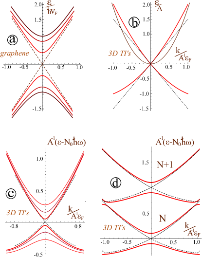
Figure 1: (Color online). Energy dispersion relations for electron dressed states. Plot (a) depicts the energy spectrum for graphene under various intensities of circularly polarized light illumination. The dashed line are for standard Dirac cone with no electron-photon interaction. Plot (b) shows the energy dispersion (red solid curves) for the effective surface model of 3D TI without light-electron interaction ($\alpha=0$, $\mathcal{D}k^{2}_{F}/(\hbar\omega_{0})=\mathcal{A}k_{F}/(\hbar\omega_{0})=0.2]$; (c) for single-mode dressed states [$\alpha=0.05$ (inner), 0.07 (middle), 0.1 (outer)] and (d) for two-mode dressed states. The dashed curves in (c) and (d) represent the asymptotic behaviors obtained by setting $\alpha=0$.

The ${\cal O}(\zeta^{2})$ correction makes an important physical difference between the dressed states in 3D TIs and graphene. However, the correction is small numerically and may be neglected in most calculations.The expression for the energy spectrum may be expressed as

$$\varepsilon^{\rm surf}_{3D}(\Delta)=N_{0}\,\hbar\omega_{0}+\mathcal{D}k^{2}+\beta\sqrt{\Delta^{2}+\left({\mathcal{A}k}\right)^{2}}\ ,$$ (20)

with $\beta=\pm 1$ and the induced energy gap defined by

$$\Delta=\sqrt{\mathcal{W}_{0}^{2}+(\hbar\omega_{0})^{2}}-\hbar\omega_{0}\sim\hbar\omega_{0}\left(\frac{\alpha^{2}}{2}\right)\ ,$$ (21)

where $\alpha=\mathcal{W}_{0}/(\hbar\omega_{0})$ and $\mathcal{W}_{0}$ is the electron-photon interaction energy. For the upper subband with $\beta=1$ in Eq. (20), the energy gap is related to the effective mass around ${\bf k}=0$ through $2m^{\ast}_{\Delta}=\hbar^{2}/\left[{\mathcal{A}^{2}/(2\Delta)+\mathcal{D}}\right]$, where the photon dressing decreases the effective mass. This is in contrast with single-layer graphene, where electron-photon interaction leads to an effective mass. A similar phenomenon on the effective mass reduction is also found in bilayer graphene under the influence of circularly polarized light. We will consider the biggest possible value for $\mathcal{W}_{0}$ to maximize the light-coupling effect, although the condition $\mathcal{W}_{0}<\hbar\omega_{0}$ must be maintained to ensure the valid approximations made in this paper. Here, as an example, we will just use the leading-order Dirac cone term ${\cal A}\,\sigma\cdot{\bf k}$ to estimate the light-induced energy gap. The small correction from the parabolic ${\cal D}$ term can be neglected for not very large $k$ values.

The dressed state wave function corresponding to Eq. (20) is given by

$$\Phi^{\bf k}_{\rm e-ph}(x,\,y)=\frac{1}{\sqrt{1+\gamma^{2}(\beta)}}\left({\begin{array}[]{c}1\\ \gamma(\beta)\texttt{e}^{i\phi}\end{array}}\right)\texttt{e}^{ik_{x}x+ik_{y}y}\ ,$$ (24)

where $\gamma(\beta)=\mathcal{A}k/[\Delta+\beta\sqrt{\Delta^{2}+(\mathcal{A}k)^{2}}]$ and $\phi=\tan^{-1}(k_{y}/k_{x})$.

In conclusion, for a single mode dressed state, the effect due to the electron-photon interaction is quite similar to graphene. The difference is that the energy gap varies as $\alpha^{2}$. However, this dependence becomes negligible under low -intensity light illumination. The energy dispersion relations for single and double-mode dressed states of 3D TIs are presented in Fig. 1. Comparing Figs. 1 (c) and (d), we find that an energy gap is opened at $k=0$ due to photon dressing, and the Dirac cone is well maintained except for large k values. In contrast, for double-mode dressed states in Fig. 1(d), additional mini-gaps appear at the Fermi edge and new saddle points are formed at $k=0$ due to strong coupling between dressed states with different pseudo-spins. These new mini-gaps and the saddle points prove to have a significant effect on electron transport and many-body properties. There exists a direct relationship between the circularly-polarized light intensity and the magnitude of energy gap $\Delta$ which is attributed to the electron-photon interaction. Here, as an example, we will just use the leading-order Dirac cone term ${\cal A}\,\sigma\cdot{\bf k}$ to estimate the light-induced energy gap. The small correction from the parabolic ${\cal D}$ term can be neglected for not very large $k$ values.

For a circular-polarized $CO_{2}$ laser beam with power $P\backsim 10^{2}\;W$, the wavelength $\lambda\backsim 10^{-5}\;m$ and the beam size on the order of $\backsim\lambda$, from the field energy density $w\backsim P/(\lambda^{2}c)$ we find the electric field amplitude $F_{0}\backsim\sqrt{P/(\epsilon_{0}\lambda^{2}c)}=10^{5}V/cm$. This leads to the light-coupling energy $W_{0}\backsim 10^{-20}\>J$ and the light-induced energy gap $\Delta\backsim 0.01-0.1\;eV$ for $Bi_{2}Se_{3}$ with $\mathcal{A}=10^{-27}\;J\;cm$.

3 Dynamical polarization and plasmons

For us to calculate the electron exchange energy, we need to obtain the non-interacting polarizability $\Pi^{0}(q,i\Omega)$ for imaginary frequency $i\Omega$ and wave number $q$. Let us consider the case of chemical potential $\mu>0$ such that the occupied electron states partially fill a finite part of the conduction band up to a certain value $\mu$. Then,

$$\Pi^{0}(q,i\Omega)=\frac{1}{\pi^{2}}\sum_{s,s^{\prime}=\pm 1}\int_{\Lambda}d^{2}k\;\mathcal{F}(\mathbf{k},\mathbf{q})\;\frac{N_{F}[\mathcal{E}_{s}(k)]-N_{F}[\mathcal{E}_{s}^{\prime}(k+q)]}{\mathcal{E}_{s}(k)-\mathcal{E}_{s}^{\prime}(k+q)+i\hbar(\Omega+\gamma)}\ ,$$ (25)

where $\gamma$ is real. The polarization function, obtained analytically in [17] for real frequencies is not suitable for our calculations. There, the only imaginary term is infinitesimal $i\gamma$. The structure factor $\mathcal{F}(k,q)$ is given as:

$$\mathcal{F}(\mathbf{k},\mathbf{q})=|\langle\Psi_{s}(k)|\Psi_{s}^{\prime}(k+q)\rangle|^{2}\ .$$ (26)

According to Eq.24, the electron dressed state wave functions may be expressed as

$$\Psi^{T}_{s}(k)=\{C_{1}(k);\;C_{2}(k)\texttt{e}^{i\theta_{k}}\}$$ (27)

and, correspondingly,

$$\Psi^{T}_{s^{\prime}}(k+q)=\{C_{1}(k+q);\;C_{2}(k+q)\texttt{e}^{i\theta_{k+q}}\}$$ (28)

so that the equation for the structure factor [26] becomes

$$\mathcal{F}(\mathbf{k},\mathbf{q})=C_{1}(k)C_{1}(k+q)+s\;s^{\prime}\;\texttt{e}^{i\delta_{\theta}}$$ (29)

with $\delta_{\theta}=\theta_{k}-\theta_{k+q}$. The prefactor, which is the squared absolute value of the wave functions overlap, now reads:

$$\mathcal{F}(\mathbf{k},\mathbf{q})=\sum_{\nu=1}^{2}\left(C_{\nu}(k)C_{\nu}(k+q)\right)^{2}+2\prod_{\xi=1}^{2}C_{\xi}(k)C_{\xi}(k+q)\;ss^{\prime}\sin\delta_{\theta}\ .$$ (30)

According to Eq. (24),

$$C_{1}(k)=\frac{\mathcal{A}k}{\sqrt{2\left(\Delta^{2}+\left(Ak\right)^{2}\right)-2\Delta\sqrt{\Delta^{2}+\left(Ak\right)^{2}}}}$$ (31)

and, correspondingly,

$$C_{2}(k)=\frac{\sqrt{\Delta^{2}+\left(Ak\right)^{2}}-\Delta}{\sqrt{2\left(\Delta^{2}+\left(Ak\right)^{2}\right)-2\Delta\sqrt{\Delta^{2}+\left(Ak\right)^{2}}\,.}}$$ (32)

As one can see, when there is no energy gap $\Delta\to 0$,

$$C_{1}=C_{2}=\frac{1}{\sqrt{2}}$$ (33)

so that the coefficients no longer depend on the wave vector $k$, and the structure factor becomes

$$\mathcal{F}_{\Delta=0}(\mathbf{k},\mathbf{q})=\frac{1}{2}\left(1+ss^{\prime}\frac{k+q\cos\phi}{|\mathbf{k}+\mathbf{q}|}\right)\,.$$ (34)

It is instructive to compare the obtained numerical results with the case of real frequency $\Omega$. Both cases are presented in Fig.2. One may conclude that the non-interacting polarization $\Pi^{0}(q,i\Omega)$ is non-zero only in a small region of $q-\Omega$ space. On the other hand, for real frequency the peak of the polarization function (both of its real and imaginary parts) is located along the main diagonal $\Omega\sim q$. The renormalized RPA polarization function is finite in a certain region and its maximum no longer represents a line of plasmons.

In the region, where undamped plasmons exist $(\Omega>\mathcal{A}q$ and $\Omega<\mu-\mathcal{A}q)$ where $\mathcal{A}$ is a constant, the real frequency polarization for interacting electrons in the RPA may be expressed as

$$\Pi(\Omega,q)=\frac{2e^{2}\mu}{\epsilon_{0}\mathcal{A}^{2}}-\frac{e^{2}\left(\mathcal{A}k\right)^{2}}{4\epsilon_{0}\sqrt{\left(\mathcal{A}k\right)^{2}+\left(\hbar\omega\right)^{2}}}\left({\mathcal{O}_{+}\sqrt{1-\mathcal{O}_{+}^{2}}+\mathcal{O}_{-}\sqrt{1-\mathcal{O}_{-}^{2}}+i\cosh^{-1}(\mathcal{O}_{+})-i\cosh^{-1}(\mathcal{O}_{-})}\right)$$ (35)

where $\mathcal{O}_{\pm}\equiv\frac{2\mu\pm\hbar\Omega}{\mathcal{A}q}$. The resulting plasmon dispersion is determined by the following identity:

$$\frac{1}{q}\Pi(\Omega_{pl},q)+\frac{2\epsilon_{0}}{e^{2}}=0\,,$$ (36)

in the long wavelength approximation resulting in [19]

$$\Omega_{pl}(q)=\left({2e^{2}\epsilon_{0}\mu\mathcal{A}\left({1-\frac{\Delta^{2}}{\mu^{2}}}\right)q}\right)^{1/2}$$ (37)

for $\Delta\to 0$ we obtained the plasmon dispersion for Dirac cone (graphene)

$$\Omega_{pl}(q)=(2e^{2}\epsilon_{0}\mu\mathcal{A}q)^{1/2}\backsim\sqrt{q}\ .$$ (38)

Clearly, the $\backsim\sqrt{q}$ dependence is similar to what we observe in 2DEG. It appears that the plasmon dispersion in 3D TIs also follow the $\backsim\sqrt{q}$ law.[20]

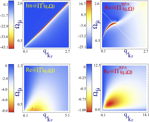
Figure 2: (Color online). Density plots for zero band gap of the polarization function for real and imaginary frequencies. The upper left panel presents the imaginary part of the non-interacting polarization function at real frequency $\Omega$. This plot shows the region where the plasmons are undamped, i.e., Im$[\Pi(q,\Omega)]=0$. The upper right plot is the real part of the interacting polarization $\Pi^{RPA}(q,\Omega)$, which shows the plasmon dispersion $\backsim\sqrt{q}$. The lower panels are the two corresponding plots for imaginary frequencies $i\Omega$. The lower left plot is the real part of the non-interacting polarizability; its imaginary part is identically zero. The lower right plot is the RPA polarization function for imaginary frequency. The plots described a gapless topological insulator.

4 Exchange energy, theory of entanglement

In this section, we calculate the exchange energy[28] as well as discuss the entanglement properties. The basic idea is that the efficiency of the electron entanglement is directly related to the exchange energy $\mathcal{E}_{ex}$. Therefore, calculating it is now our goal since we may then confine electrons to quantum dots[29] for the purpose of using entangled spins in applications such as quantum computing and sensors.

The general formula for the electron exchange energy in 3D is[30, 31]

$$\mathcal{E}_{ex}=-\frac{A}{2}\int d^{3}\mathbf{r}\int d^{3}\mathbf{r^{\prime}}\ V(|\mathbf{r}-\mathbf{r^{\prime}}|)\left({\frac{1}{\pi}\int_{0}^{\infty}d\omega\Pi^{0}(\mathbf{r},\mathbf{r^{\prime}},i\Omega)+n(\mathbf{r})\delta(\mathbf{r}-\mathbf{r^{\prime}})}\right)$$ (39)

where $A$ is a normalization area, $V(|\mathbf{r}-\mathbf{r^{\prime}}|)$ is the Coulomb interaction and $n(\mathbf{r})$ is electron number density. After a 2D Fourier transformation along the $x-$ and $y-$ axes, we obtain

$$\mathcal{E}_{ex}=-\frac{A}{2}\int d\mathbf{k}_{\parallel}\int_{0}^{\infty}dz\int_{0}^{\infty}dz^{\prime}V(\mathbf{k}_{\parallel},z-z^{\prime})\left[{\frac{1}{\pi}\int_{0}^{\infty}d\Omega\Pi^{0}(\mathbf{k}_{\parallel},z,z^{\prime};i\Omega)+n_{av}(z)\delta(z-z^{\prime})}\right]$$ (40)

with $n_{av}(z)=(1/A)\int dx\,dy\,\ n(x,y,z)$. For a purely 2D system, Eq.39 becomes

$$\mathcal{E}_{ex}^{surf}=-\frac{A}{2}\int_{-\infty}^{\infty}dq_{x}\int_{-\infty}^{\infty}dq_{y}\ V(\mathbf{q})\left[\frac{1}{\pi}\int_{0}^{\infty}d\Omega\ \Pi^{0}(\mathbf{q},i\Omega)+n_{av}\right]$$ (41)

here $n_{av}=(1/A)\int dx\,dy\,\ n(x,y)$ is the 2D electron density.The $d^{2}q$ integral diverges only for $n_{av}=0$, which we will accept for the rest of our calculations.

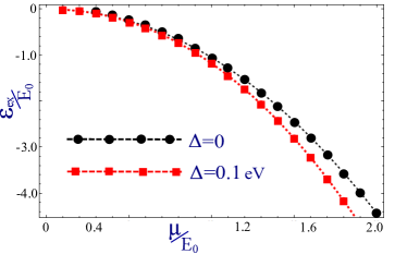
Figure 3: (Color online). Electron exchange energy as a function of chemical potential. The black line corresponds to the case of gapless energy dispersion and the red line is for energy gap $\Delta=0.9\mu$. $E_{0}\backsimeq 1\;eV$ is an energy constant, determined from the integration cut off.

The correlation energy for both graphene[32] and TI may be obtained with the use of the PRA polarization for imaginary frequencies. The correlation leads to the spin and charge susceptibilities being suppressed for chiral Dirac cone in both graphene and 3D TIs

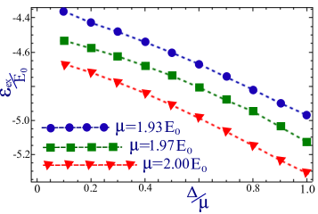
Figure 4: (Color online). Exchange energy is plotted as a function of the energy gap, for chosen chemical potential. The gap for the electron energy dispersion is scaled with the chemical potential. Each line corresponds to certain level of electron doping, and the and the difference is a few percent. This shows that the chemical potential has much stronger influence on the exchange compared to energy gap.

The obtained variation of the exchange energy is presented in Figs. [3 It has been argued that the entanglement is determined by the electron exchange energy [21, 22]. The entanglement of the electron spins in the channels driven by the surface acoustic waves was considered in [23]   .

5 Concluding Remarks

In summary, we have calculated the exchange energy for electron-photon dressed effective surface states for 3D TIs. The dressed states, which appear as a result of the electron interaction with circularly polarized light, lead to the existence of a finite gap in the energy dispersion and breaking of the chiral symmetry of the corresponding wave function. The energy gap, which may be as large as $0.1$ eV for circularly-polarized laser beam of $10^{2}$ W power. This may exceeds the geometrical energy gap which appears if a 3D TI sample has a finite width.

The circular polarization of the imposed light allows complete analytic solution for both graphene and TIs due to the fact that for $k=0$ each Hamiltonian coincides with that for the Jayness-Cummings model and the corresponding eigenstates are used as a basis of the expansion of the wave functions.

The obtained dressed states in TIs acquire an energy gap like graphene. However, unlike graphene, the electron-photon interaction has significant influence on the valence (lower) subband. In the case of a higher interaction amplitude, the hole-subband becomes nearly dispersionless. As far as gap is concerned, its value is large compared to the case of the electron dressed states in grpahene, but the difference is not important or of significant value.

We have calculated numerically the non-interacting polarization function with both real and imaginary frequencies. The latter quantity $\Pi(q,i\Omega)$ enters into the expression for the exchange energy and the real $\Omega$ polarization together with the RPA polarization determine the plasmon dispersion as well as the region where undamped plasmons could exist. Our calculations of the real-$\Omega$ polarization completely agree with the earlier obtained results for the plasmonics [17, 19].

It has been argued that the electron exchange energy has a direct and strong influence on the entanglement. This has been considered for both quantum dots and channels, originating from surface acoustic waves. We concluded that the doping value (chemical potential) has a strong influence on the exchange energy and, as a consequence, on the electron entanglement. We have also found that the energy gap, due to the electron-photon interaction leads to an increase in the magnitude of the electron exchange energy. However, this dependence is much weaker compared to the $\mu-$dependence. As a result, we propose a technique to tune and control the electron entanglement by both the chemical potential and the electron-photon interaction, so that the second mechanism may be used for a small tuning which we believe has a strong potential for device applications.

References

- [1] B. Bernevig, T. A. Hughes, and S.-C. Zhang, “Quantum spin hall effect and topological phase transition in hgte quantum wells,” Science 314, pp. 1751–1761, Dec. 2006.
- [2] M. König, S. Wiedmann, C. Brüne, A. Roth, H. Buhmann, L. W. Molenkamp, X.-L. Qi, and S.-C. Zhang, “Quantum spin hall insulator state in hgte quantum wells,” Science 318(5851), pp. 766–770, 2007.
- [3] M. Z. Hasan and C. L. Kane, “Colloquium : Topological insulators,” Rev. Mod. Phys. 82, pp. 3045–3067, Nov 2010.
- [4] X.-L. Qi and S.-C. Zhang, “Topological insulators and superconductors,” Rev. Mod. Phys. 83, pp. 1057–1110, Oct 2011.
- [5] J.W.Mclver and et al., “Control over topological insulator photocurrents with light polarization,” Nature Nanotech. 7, p. 96, 2011.
- [6] B. Zhou, H.-Z. Lu, R.-L. Chu, S.-Q. Shen, and Q. Niu, “Finite size effects on helical edge states in a quantum spin-hall system,” Phys. Rev. Lett. 101, p. 246807, Dec 2008.
- [7] W.-Y. Shan, H.-Z. Lu, and S.-Q. Shen, “Effective continuous model for surface states and thin films of three-dimensional topological insulators,” New Journal of Physics 12(4), p. 043048, 2010.
- [8] T. Oka and H. Aoki, “Photovoltaic hall effect in graphene,” Phys. Rev. B 79(8), p. 081406, 2009.
- [9] T. Kitagawa, T. Oka, A. Brataas, L. Fu, and E. Demler, “Transport properties of nonequilibrium systems under the application of light: Photoinduced quantum hall insulators without landau levels,” Phys. Rev. B 84, p. 235108, Dec 2011.
- [10] B. Dóra, J. Cayssol, F. Simon, and R. Moessner, “Optically engineering the topological properties of a spin hall insulator,” Phys. Rev. Lett. 108, p. 056602, Jan 2012.
- [11] N. H. Linder, D. L.Bergman, G. Rafael, and V. Galitski, “Topological floquet spectrum in three dimensions vis a two-photon resonance,” arXiv:1111.4518 , Feb. 2012.
- [12] S. Roche and L. E. F. Torres, “On the possibility of observing tunable laser-induced bandgaps in graphene,” Graphene, Carbon Nanotubes, and Nanostuctures: Techniques and Applications 12, p. 41, 2013.
- [13] E. Suárez Morell and L. E. F. Foa Torres, “Radiation effects on the electronic properties of bilayer graphene,” Phys. Rev. B 86, p. 125449, Sep 2012.
- [14] H. L. Calvo, P. M. Perez-Piskunow, H. M. Pastawski, S. Roche, and L. E. F. Torres, “Non-perturbative effects of laser illumination on the electrical properties of graphene nanoribbons,” Journal of Physics: Condensed Matter 25(14), p. 144202, 2013.
- [15] H. L. Calvo, P. M. Perez-Piskunow, S. Roche, and L. E. Foa Torres, “Laser-induced effects on the electronic features of graphene nanoribbons,” Applied Physics Letters 101(25), pp. 253506–253506, 2012.
- [16] A. Iurov, G. Gumbs, O. Roslyak, and D. Huang, “Photon dressed electronic states in topological insulators: tunneling and conductance,” Journal of Physics: Condensed Matter 25(13), p. 135502, 2013.
- [17] B. Wunsch, T. Stauber, F. Sols, and F. Guinea, “Dynamical polarization of graphene at finite doping,” New Journal of Physics 8(12), p. 318, 2006.
- [18] E. H. Hwang and S. Das Sarma, “Dielectric function, screening, and plasmons in two-dimensional graphene,” Phys. Rev. B 75, p. 205418, May 2007.
- [19] P. Pyatkovskiy, “Dynamical polarization, screening, and plasmons in gapped graphene,” Journal of Physics: Condensed Matter 21(2), p. 025506, 2009.
- [20] D. Efimkin, Y. Lozovik, and A. Sokolik, “Spin-plasmons in topological insulator,” Journal of Magnetism and Magnetic Materials 324(21), pp. 3610 – 3612, 2012.
- [21] C. H. W. Barnes, J. M. Shilton, and A. M. Robinson, “Quantum computation using electrons trapped by surface acoustic waves,” Phys. Rev. B 62, pp. 8410–8419, Sep 2000.
- [22] G. Burkard, D. Loss, and D. P. DiVincenzo, “Coupled quantum dots as quantum gates,” Phys. Rev. B 59, pp. 2070–2078, Jan 1999.
- [23] G. Gumbs and Y. Abranyos, “Quantum entanglement for acoustic spintronics,” Phys. Rev. A 70, p. 050302, Nov 2004.
- [24] O. V. Kibis, “Metal-insulator transition in graphene induced by circularly polarized photons,” Phys. Rev. B 81(16), p. 165433, 2010.
- [25] O. V. Kibis, O. Kyriienko, and I. A. Shelykh, “Band gap in graphene induced by vacuum fluctuations,” Phys. Rev. B 84, p. 195413, Nov 2011.
- [26] A. Iurov, G. Gumbs, O. Roslyak, and D. Huang, “Anomalous photon-assisted tunneling in graphene,” Journal of Physics: Condensed Matter 24(1), p. 015303, 2012.
- [27] D. Culcer, E. H. Hwang, T. D. Stanescu, and S. Das Sarma, “Two-dimensional surface charge transport in topological insulators,” Phys. Rev. B 82, p. 155457, Oct 2010.
- [28] G. Gumbs, “Correlation energy of a one-component layered electron gas,” Phys. Rev. B 40, pp. 5788–5791, Sep 1989.
- [29] O. Roslyak, G. Gumbs, and S. Mukamel, “Trapping photon-dressed dirac electrons in a quantum ot studied by coherent two dimensional photon echo spectroscopye,” Journal of Chemical Physics 136, p. 194106, 2012.
- [30] J. Harris and R. O. Jones, “The surface energy of a bounded electron gas,” Journal of Physics F: Metal Physics 4(8), p. 1170, 1974.
- [31] A. Griffin, J. Harris, and H. Kranz, “Normal modes and the rpa correlation energy of a metallic film,” Journal of Physics F: Metal Physics 4(10), p. 1744, 1974.
- [32] Y. Barlas, T. Pereg-Barnea, M. Polini, R. Asgari, and A. H. MacDonald, “Chirality and correlations in graphene,” Phys. Rev. Lett. 98, p. 236601, Jun 2007.