Interaction quenches in the 1D Bose gas

Abstract

The non-equilibrium dynamics of integrable systems are special: there is substantial evidence that after a quantum quench they do not thermalize but their asymptotic steady state can be described by a Generalized Gibbs Ensemble (GGE). Most of the studies on the GGE so far have focused on models that can be mapped to quadratic systems while analytic treatment in non-quadratic systems remained elusive. We obtain results on interaction quenches in a non-quadratic continuum system, the 1D Bose gas described by the integrable Lieb–Liniger model. We compute local correlators for a non-interacting initial state and arbitrary final interactions as well as two-point functions for quenches to the Tonks–Girardeau regime. We show that in the long time limit integrability leads to significant deviations from the predictions of the grand canonical ensemble.

Whether and how an isolated quantum system equilibrates or thermalizes are fundamental questions in understanding non-equilibrium dynamics. The answers can also shed light on the applicability of quantum statistical mechanics to closed systems. While these questions are very hard to study experimentally in the condensed matter setup, they have become accessible in ultracold quantum gases due to recent experimental advances review . Thanks to their unprecedented tunability, ultracold atomic systems allow for the study of non-equilibrium quantum dynamics of almost perfectly isolated strongly correlated many-body systems in a controlled way. These experiments kinoshita ; greiner ; hofferberth ; trotzky ; cheneau ; gring ; haller ; schneider ; ronzheimer triggered a revival of theoretical studies on issues of thermalization rev ; rigorous ; cardycalabrese ; quench ; LLquench ; ising ; luttinger ; GGE ; gge_various ; gge_non2 ; fioretto ; mossel ; local ; js-fabian ; truncGGE . The list of fundamental questions include whether stationary values of local correlation functions are reached in a system brought out of equilibrium, and if so, how they can be characterized. Can conventional statistical ensembles describe the state? Is there any kind of universality in the steady state and the way it is approached?

The absence of thermalization of a 1D bosonic gas reported in Ref. kinoshita brought to light the special role of integrability. The observed lack of thermalization was attributed to the fact that the system was very close to an integrable one, the Lieb–Liniger (LL) model LL which is the subject of our Letter. The dynamics of integrable systems are highly constrained by the presence of a large number of conserved charges sutherland in addition to the total particle number, momentum, and energy, thus they are not expected to thermalize. The so-called Generalized Gibbs Ensemble (GGE) was proposed GGE to capture the long-time behavior of integrable systems brought out of equilibrium. The density matrix is

$$\hat{\rho}_{\text{GGE}}=\frac{e^{-\sum_{m}\beta_{m}\hat{Q}_{m}}}{Z_{\text{GGE}}}\,,$$ (1)

where the generalized “chemical potentials” $\{\beta_{m}\}$ are fixed by the expectation values ${\langle\hat{Q}_{m}\rangle}$ in the initial state, and $Z_{\text{GGE}}=\mathrm{Tr}\left[e^{-\sum_{m}\beta_{m}\hat{Q}_{m}}\right]$. The GGE proposal was tested successfully by various numerical and analytic approaches gge_various ; gge_non2 ; fioretto ; mossel .

Recently, locality has emerged as a crucial ingredient in the understanding of equilibration and the meaning of a steady state local . While the whole system starting in an initial pure state clearly cannot evolve into a mixed state, its subsystems are fully described by a reduced density matrix obtained by tracing out the rest of the system that acts as a bath for the subsystem. There is substantial evidence that this density matrix is thermal for generic systems and given by the GGE for integrable systems. Naturally, it is the local conserved charges that are to be used in the GGE density matrix.

The GGE was studied mostly in models which can be mapped to quadratic bosonic or fermionic systems where the conserved charges are given by the mode occupation numbers. While some of these models are paradigmatic, like the Ising or Luttinger models, a prominent class of non-trivial integrable systems has not been sufficiently explored, namely those solvable by the Bethe Ansatz (BA). In these models, the local conserved charge operators are usually known but cannot be expressed as mode occupations.

The work fioretto focused on integrable quantum field theories and demonstrated that the long-time limit of expectation values are given by a GGE, assuming a special initial state. In Ref. js-fabian it was shown for BA integrable models that in the thermodynamic limit the time evolution of local observables after a quantum quench is captured by a saddle point state, and their $t\to\infty$ asymptotic values are given by their expectation values in this state. The saddle point state can be determined using the expectation values of the charges in the initial state.

In this Letter, we focus on a BA solvable continuum model: we derive experimentally testable predictions for the long time behavior of the LL model after an interaction quench LLquench combining Bethe Ansatz methods and GGE. For a non-interacting initial state and arbitrary final interactions we calculate expectation values of point-localized operators, while for quenches to the fermionized Tonks–Girardeau regime we obtain exact results on two-point correlation functions.

The model.—

The LL model describes a system of identical bosons in 1D interacting via a Dirac-delta potential. The Hamiltonian is given by LL

$$\hat{H}=-\sum_{i}^{N}\frac{\partial^{2}}{\partial x_{i}^{2}}+2c\sum_{i<j}\,\delta(x_{i}-x_{j})\,,$$ (2)

which in the second quantized formulation takes the form

$$\hat{H}=\int_{0}^{L}\mathrm{d}x\,\left(\partial_{x}\hat{\psi}^{\dagger}\partial_{x}\hat{\psi}+c\,\hat{\psi}^{\dagger}\hat{\psi}^{\dagger}\hat{\psi}\hat{\psi}\right)\,,$$ (3)

where $c>0$ in the repulsive regime we wish to study, and for brevity we set $\hbar=1$ and the boson mass to be equal to $1/2$. The dimensionless coupling constant is given by $\gamma=c/n$, where $n=N/L$ is the density of the gas. In cold atom experiments $\gamma$ is a function of the 3D scattering length and the 1D confinement olshanii . The exact spectrum and thermodynamics of the model can be obtained via Bethe Ansatz LL ; KBI . The many-body eigenfunctions $\phi(\{x_{i}\})$ of $\hat{H}$ satisfy the boundary condition

$$\left.\left(\frac{\partial}{\partial x_{j}}-\frac{\partial}{\partial x_{k}}-c\right)\phi(x_{1},\dots,x_{N})\right|_{x_{j}=x_{k}+0}=0\,,$$ (4)

whenever the coordinates of two particles coincide, thus the wave functions have cusps. The eigenstates on a ring can be expressed in terms of $N$ quasimomenta $\{\lambda_{j}\}$ that satisfy a set of algebraic equations, the Bethe equations. The eigenvalues of the mutually commuting local conserved charges can be computed as ${\langle\hat{Q}_{m}\rangle}=\sum_{j}\lambda_{j}^{m},$ in particular, the energy is simply $E={\langle\hat{Q}_{2}\rangle}=\sum_{j}\lambda_{j}^{2}$ KBI . In the thermodynamic limit (TDL), a mixed state is captured by a continuous density of quasimomenta, $\rho_{\text{LL}}(\lambda)$yang . All quasimomenta are coupled to each other by the Bethe equations and thus $\rho_{\text{LL}}(\lambda)$ as well as the density of “holes” satisfies integral equations, the Thermodynamic Bethe Ansatz (TBA) equations. This approach was developed for thermal equilibrium but it can be generalized to the case of the GGE mossel .

Divergence of the local conserved charges.—

The simplest way to bring a system out of equilibrium is a sudden change of one of its parameters, a quantum quench cardycalabrese . In a cold atom setting such a quench could be achieved by a rapid change of the transverse confinement or the scattering length. We will compute the predictions of the GGE for a sudden quench of the interaction parameter $c$ starting from the ground state of the $c=0$ system, a pure non-interacting BEC (although we expect our results to be also valid for small initial interactions) and compare them with those of the grand canonical ensemble (GCE).

In order to describe the final state in terms of the distribution $\rho_{\text{LL}}(\lambda)$, one needs to find the expectation values of the conserved charges $\hat{Q}_{m}$ right after the quench, i.e. in the BEC-like ground state of free bosons. The density $\rho_{\text{LL}}(\lambda)$ is then found, in principle, by solving the problem of moments defined by ${\langle\hat{Q}_{m}\rangle}=L\int\mathrm{d}\lambda\,\rho_{\text{LL}}(\lambda)\,\lambda^{m}.$ The first few $\hat{Q}_{m}$ can be written in terms of the field operator as $\hat{Q}_{0}=\int\mathrm{d}x\,\hat{\psi}^{\dagger}\hat{\psi},$ $\int\hat{Q}_{1}=-i\int\mathrm{d}x\,\hat{\psi}^{\dagger}\partial_{x}\hat{\psi},$ and $\hat{Q}_{2}=\hat{H}$ is the Hamiltonian given by Eq. (3). Unfortunately, similar second quantized expressions do not exist for the operators $\hat{Q}_{m}$ for $m\geq 4$ davies . More importantly, their expectation values can be shown to diverge in almost all states other than the eigenstates of $\hat{H}.$ The reason is that their first quantized expressions contain products of Dirac deltas and higher derivatives davies ; jornthesis , and are only meaningful when evaluated on a wave function satisfying the cusp condition (4). Clearly, any eigenfunction of the Hamiltonian with a different coupling $c$, including the BEC wave function, will violate this condition Note that although its expectation value is finite, even the action of the Hamiltonian is singular on such a state as it generates Dirac-$\delta$’s . The diverging expectation values of the charges imply in general that the density $\rho_{\text{LL}}(\lambda)$ has a $\lambda^{-4}$ power-law tail instead of the usual exponential fall-off. We expect these divergences to be a generic phenomenon for interaction quenches in continuum models which has not been addressed so far.

q-boson regularization.—

To circumvent the problem of divergences we regularize them by considering an integrable lattice regularization of the LL model, the so-called $q$-boson hopping model qboson . The Hamiltonian is

$$H_{q}=-\frac{1}{\delta^{2}}\sum_{j=1}^{M}(B_{j}^{\dagger}B_{j+1}+B_{j+1}^{\dagger}B_{j}-2N_{j})\,,$$ (5)

where $\delta$ is the lattice spacing of the lattice of length $M$ having periodic boundary conditions. The operators $B_{j},$ $B_{j}^{\dagger}$ and the number operator $N_{j}=N^{\dagger}_{j}$ satisfy the $q$-boson algebra

$$B_{j}B_{j}^{\dagger}-q^{-2}B_{j}^{\dagger}B_{j}=1\,,\quad q>1,$$ (6)

with $[N_{j},B_{j}]=-B_{j}$, $[N_{j},B_{j}^{\dagger}]=B_{j}^{\dagger},$ and operators at different sites commute. In the representation on the Fock space generated by the canonical lattice boson operators $b_{j},b^{\dagger}_{j}$ at each site it is possible to express the $q$-operators as $N_{j}=b_{j}^{\dagger}b_{j},$ $B_{j}=\sqrt{\frac{[N_{j}+1]_{q}}{N_{j}+1}}\,b_{j},$ where $[x]_{q}\equiv\frac{1-q^{-2x}}{1-q^{-2}}.$ Note that as $q\to 1$, $[x]_{q}\to x$ and therefore $B^{(\dagger)}_{j}\to b^{(\dagger)}_{j}.$ The Hamiltonian is non-polynomial either in the $b$ or the $B$ operators, thus the model is interacting and the interaction is encoded in the deformation parameter $q.$ In the naive limit $q\to 1$ we recover the system free bosons hopping on a lattice. We are interested instead in the following continuum limit: let $\delta\to 0,$ $M\to\infty,$ and $q\to 1,$ while $L$ and $c$ are kept constant:

$$L=M\delta\,,\;\;c/2=\kappa\delta^{-1}\,,\text{ as }M\to\infty\text{ and }\delta,\kappa\to 0\,,$$ (7)

where $\kappa$ is related to $q$ as $q=e^{\kappa}.$ Defining the continuum boson fields $\hat{\psi}(x=j\delta)=\delta^{-1/2}b_{j},$ the $q$-boson Hamiltonian (5) becomes the LL Hamiltonian in the limit (7).

The main idea behind our regularized GGE is to use the local conserved charges of the lattice model to determine the density of quasimomenta of $q$-bosons first, and to take the continuum limit yielding $\rho_{\text{LL}}(\lambda)$ only as the last step. An infinite set of mutually commuting local charges can be constructed via the Quantum Inverse Scattering Method epaps . They are of the form $I_{m}=\delta\sum_{j=1}^{M}\mathcal{J}^{(m)}_{j},$ where the operators $\mathcal{J}^{(m)}_{j}$ act nontrivially in $m+1$ neighboring lattice sites only. These charges are not in one-to-one correspondence with the LL operators $\hat{Q}_{m}$.

Similarly to the LL model, the common eigenstates of all $I_{m}$ are defined in the $N$-particle sector by $N$ quasi-momenta $\{p_{i}\}$ which are solutions of the $q$-boson Bethe equations. Under the limit (7) the quasi-momenta should be rescaled as $\lambda_{j}=p_{j}/\delta$ in order to regain the Bethe equations of the LL model. In the thermodynamic limit, $N,M\to\infty,$ $\nu\equiv N/M=\text{const.}$, we introduce the quasimomentum distribution function $\rho_{q}(p)$. In terms of $\rho_{q}(p)$ the expectation values of the integrals of motion can be written as CHZ

$$\rho_{m}\equiv\frac{|m|\langle I_{m}\rangle}{M\left(1-q^{-2|m|}\right)}=\int_{-\pi}^{\pi}\cos{(mp)}\rho_{q}(p)\mathrm{d}p\,,$$ (8)

for $m=1,2,\dots$, and $\rho_{0}=\nu$, thus the expectation values are essentially the Fourier series coefficient of $\rho_{q}(p).$ Here we specialized to the case where the parity symmetry is not broken and thus $\rho_{q}(p)$ is an even function.

The density $\rho_{\text{LL}}(\lambda)$.—

Let us evaluate now expectation values of $I_{m}$ in a $q$-boson state which reduces to the free boson ground state in the continuum limit, i.e. a BEC state. There is no unique choice but we pick the lattice BEC state $|\text{BEC}\rangle_{N}=\frac{1}{\sqrt{N!}}\left(\frac{1}{\sqrt{M}}\sum_{i}b^{\dagger}_{i}\right)^{N}|0\rangle,$ where $b^{\dagger}_{i}$ are creation operators of canonical lattice bosons. Using the explicit expressions of the charge densities $\mathcal{I}^{(m)}_{j}$ in terms of the $B^{(\dagger)}_{j}$ operators, expanding these in terms of $b^{(\dagger)}_{j}$ we obtain series expansions of ${\langle I_{m}\rangle}$ in terms of the small parameter $\kappa$ epaps . Combining the lowest orders of the first few ${\langle I_{m}\rangle}$ we confirmed that we obtain the correct value of energy in the limit, $E/L=n^{3}\gamma$. We also find that in the continuum limit $\hat{Q}_{4}$ is divergent, as expected epaps .

Based on the first seven charges we conjectured a pattern for the lowest orders in the expansion of the expectation values epaps . The distribution $\rho_{q}(p)$ is obtained by taking the Fourier sum, $\rho_{q}(p)=\frac{1}{2\pi}\sum_{m=-\infty}^{\infty}\rho_{m}\cos(mp)$. Summing up the Fourier series order by order in $\kappa$ and then taking the continuum limit we find

$$2\pi\rho_{\text{LL}}(\lambda)=\frac{n^{4}\gamma^{2}}{\lambda^{4}}-\frac{n^{6}\gamma^{3}(\gamma-24)}{4\lambda^{6}}+\dots\,.$$ (9)

The expansion of the Fourier modes $\rho_{m}$ in terms of $\kappa$ translates into a large momentum expansion of $\rho_{\text{LL}}(\lambda)$ due to the rescaling of momenta, $\lambda=p/\delta$. We found the expected $\lambda^{-4}$ tail together with the subleading $\lambda^{-6}$ tail.

To find the full $\rho_{\text{LL}}(\lambda)$ function one needs a pattern for the $\rho_{m}$ in all orders in $\kappa$. This requires the knowledge of the expectation values of higher charges which are increasingly hard to the compute. However, for observables localized on $l$ neighboring sites the truncated GGE using the first $m\gtrsim l$ charges of size $\leq m+1$ is expected to give a very good approximation XXZ . Observables localized at a point in the LL model, like $g_{k}={\langle:\!(\hat{\psi}(x)^{\dagger}\hat{\psi}(x))^{k}\!:\rangle}/n^{k}$, are the limits of operators localized on a few neighboring sites in the $q$-boson lattice system, thus we expect to capture the $g_{k}$ using the first few conserved $q$-boson charges.

To this end, we approximate $\rho_{q}(p)$ by the truncated Fourier sum using the Fourier–Padé approximation. Keeping charges up to $I_{4}$ and $I_{5}$, Padé-approximants of different types yield the same result in the limit epaps :

$$\rho^{(1)}_{\text{LL}}(\lambda)=\frac{1}{2\pi}\frac{\gamma^{2}}{(\lambda/n)^{4}+\gamma(\gamma/4-2)(\lambda/n)^{2}+\gamma^{2}}\,.$$ (10)

This result changes only when we take into account $I_{6}$: it becomes the ratio of a second and a sixth order polynomial in $\lambda$, which we call $\rho_{\text{LL}}^{(2)}(\lambda)$ epaps . The densities are shown for $\gamma=1$ in the inset of Fig. 1 together with the GCE density fixed by the energy and particle number only. Let us note that, interestingly, the $\gamma\to\infty$ limit of both expressions gives the Lorentzian form

$$\lim_{\gamma\to\infty}\rho^{(1,2)}_{\text{LL}}(\lambda)=\frac{1}{2\pi}\frac{4}{(\lambda/n)^{2}+4}\,.$$ (11)

Correlation functions in the final state.—

Knowing the density $\rho_{\text{LL}}(\lambda)$ allows us to calculate correlation functions. First we compute point-local correlators using the results of Ref. g3 which give analytic expressions for the local two and three-point correlators for arbitrary states that are captured by a continuous $\rho_{\text{LL}}(\lambda)$. We compute $g_{2}={\langle:\!(\hat{\psi}^{\dagger}\hat{\psi})^{2}\!:\rangle}/n^{2}$ and $g_{3}={\langle:\!(\hat{\psi}^{\dagger}\hat{\psi})^{3}\!:\rangle}/n^{3}$ both for the GGE and the GCE by using the appropriate $\rho_{\text{LL}}(\lambda)$. In the latter only the energy and the particle densities are fixed to be the same as for the GGE. The results are shown in the main panel of Fig. 1. The values of the correlators computed using the two Padé approximants are very close to each other conforming with the expectation that adding more charges to the thermal GGE does not significantly change the result. This is an important consistency check of our truncation method. The deviations are bigger for $g_{3}$ which agrees with the intuition that $g_{3}$ is more complex than $g_{2}$. The second observation is that as the difference between the two truncated results decreases for increasing $\gamma$, their deviation from the GCE results $g_{k}^{\text{th}}$ (dotted lines) grows, the relative difference between the $g_{2}$ values being bigger than $20\%$ for $\gamma>10$. For strong interactions the asymptotic behavior of $g_{k}$ can be obtained analytically. For $g_{2}$ we find $g_{2}\sim 8/(3\gamma)$ and $g_{2}^{\text{th}}\sim 4/\gamma$ implying a factor of $3/2$ between the two. For $g_{3}$ even the power laws are different: $g_{3}\sim 32/(15\gamma^{2})$ while $g_{3}^{\text{th}}\sim 72/\gamma^{3}$.

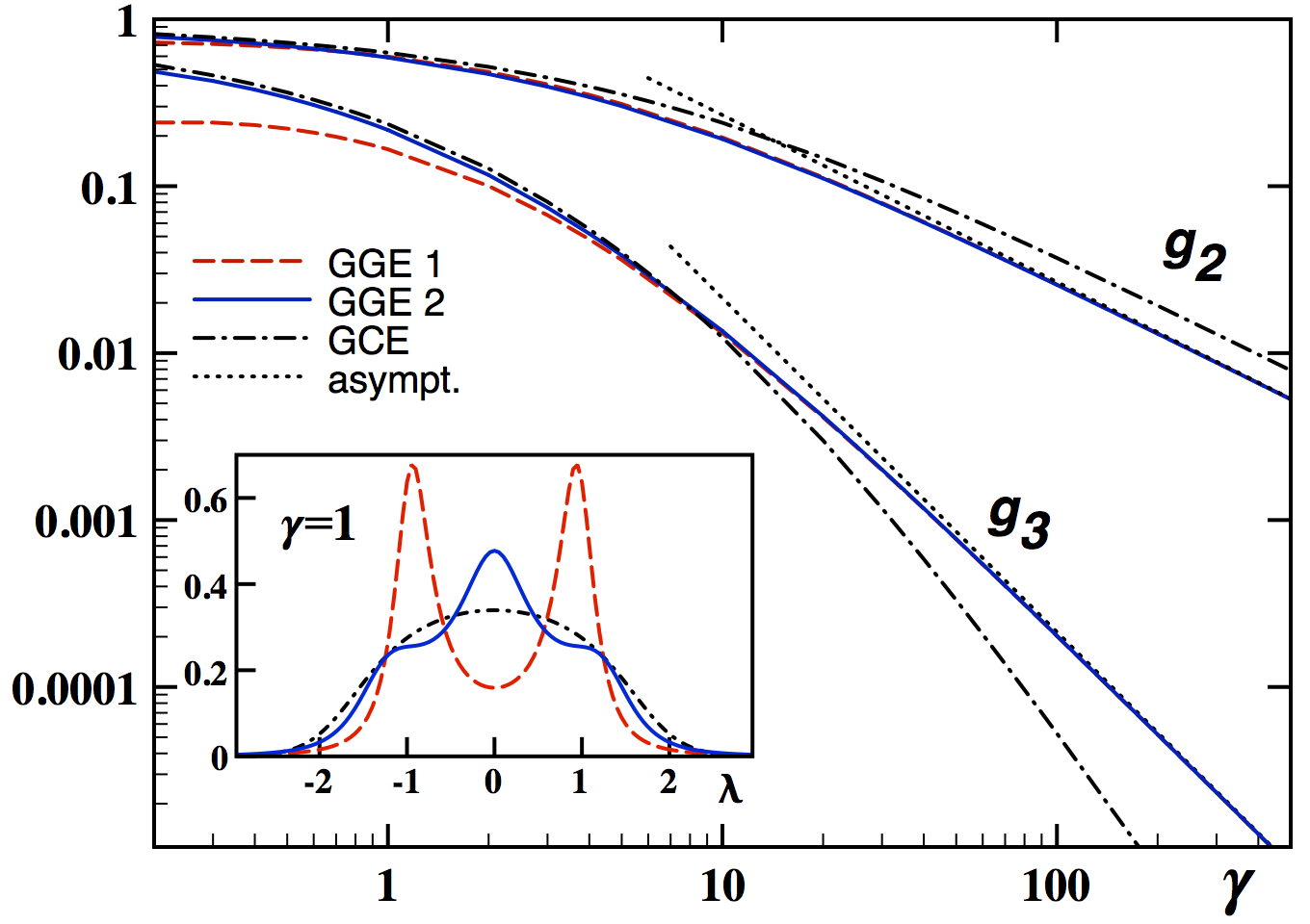
Figure 1: Quench from a non-interacting initial state to arbitrary final interactions. Main panel: Local correlations $g_{2}$ and $g_{3}$ as functions of the coupling $\gamma$, calculated from the two truncated Generalized Gibbs Ensembles (GGE) (red dashed, blue solid) and from the grand canonical ensemble (GCE) (dot-dashed). The asymptotic behaviors are also shown (dotted). Inset: density of quasimomenta, $\rho_{\text{LL}}^{(1)}(\lambda),\rho_{\text{LL}}^{(2)}(\lambda)$ in the two truncated GGE (red dashed, blue solid) and $\rho_{\text{LL}}^{\text{th}}(\lambda)$ in the GCE (black dot-dashed) for $\gamma=1.$

Strongly interacting final state.—

For large coupling the system is in the fermionized TG regime since the strong repulsion induces an effective Pauli principle in real space. In the special case of the quench from $c=0$ to $c=\infty$ the overlaps between the initial state and the final TG eigenstates are explicitly known gritsev . Only states defined by a set of $\{\lambda_{i},-\lambda_{i}\}$ pairs have nonzero overlaps which are $\langle{\lambda_{i}}|\text{BEC}\rangle\propto 1/\prod_{\lambda_{i}>0}\lambda_{i}$. The overlaps are the necessary ingredients in the formalism of Ref. js-fabian to compute the saddle point density. Solving the generalized TBA equations we obtain the simple result $2\pi\rho_{\text{LL}}(\lambda)=1/(1+\lambda^{2}n^{2}/4)$ (see also Ref. j-s ) which exactly matches the $\gamma\to\infty$ limit of our Padé-approximants, Eq. (11). The fact that the two derivations are completely independent gives a strong evidence for the correctness of the result.

Bosonic correlation functions can now be calculated by first fermionizing the field operators using Jordan–Wigner strings, $\hat{\psi}(x)=\exp[i\pi\int_{-\infty}^{x}\hat{\psi}^{\dagger}_{\text{F}}(z)\hat{\psi}_{\text{F}}(z)dz]\hat{\psi}_{\text{F}}(x)$, and then exploiting free fermionic correlators of $\hat{\psi}_{\text{F}}$. Let us consider the equal time correlation $G(x)=\langle\hat{\psi}^{\dagger}(x)\hat{\psi}(0)\rangle$ in the saddle point distribution of Eq. (11). After introducing a lattice discretization, the long chain of operators is amenable to a Wick expansion using as a building block the fermionic two point function. Since for $\gamma=\infty$ the quasimomenta coincide with the physical momenta, this is given by the Fourier transform of the density (11), $G_{\rm FF}(x)=\int\mathrm{d}\lambda\rho_{\text{s}}(\lambda)e^{i\lambda x}=e^{-2n|x|}.$ The Wick expansion can be recast as a Fredholm-like determinant ripplezvon that finally leads to $G(x)=e^{-2n|x|}$. This simple result is drastically different from the corresponding GCE result, $G_{\text{th}}(x)\stackrel{{\scriptstyle\gamma\to\infty}}{{\longrightarrow}}e^{-\gamma(nx)^{2}/2}$, which approaches an infinitely narrow Dirac-$\delta$ in the TG limit. Since $G(x)=G_{\text{FF}}(x)$, the experimentally accessible bosonic momentum distribution, $n_{\text{B}}(k)$, is thus equal to $\rho_{\text{LL}}(k)$ given by Eq. (11), plotted in the inset of Fig. 2.

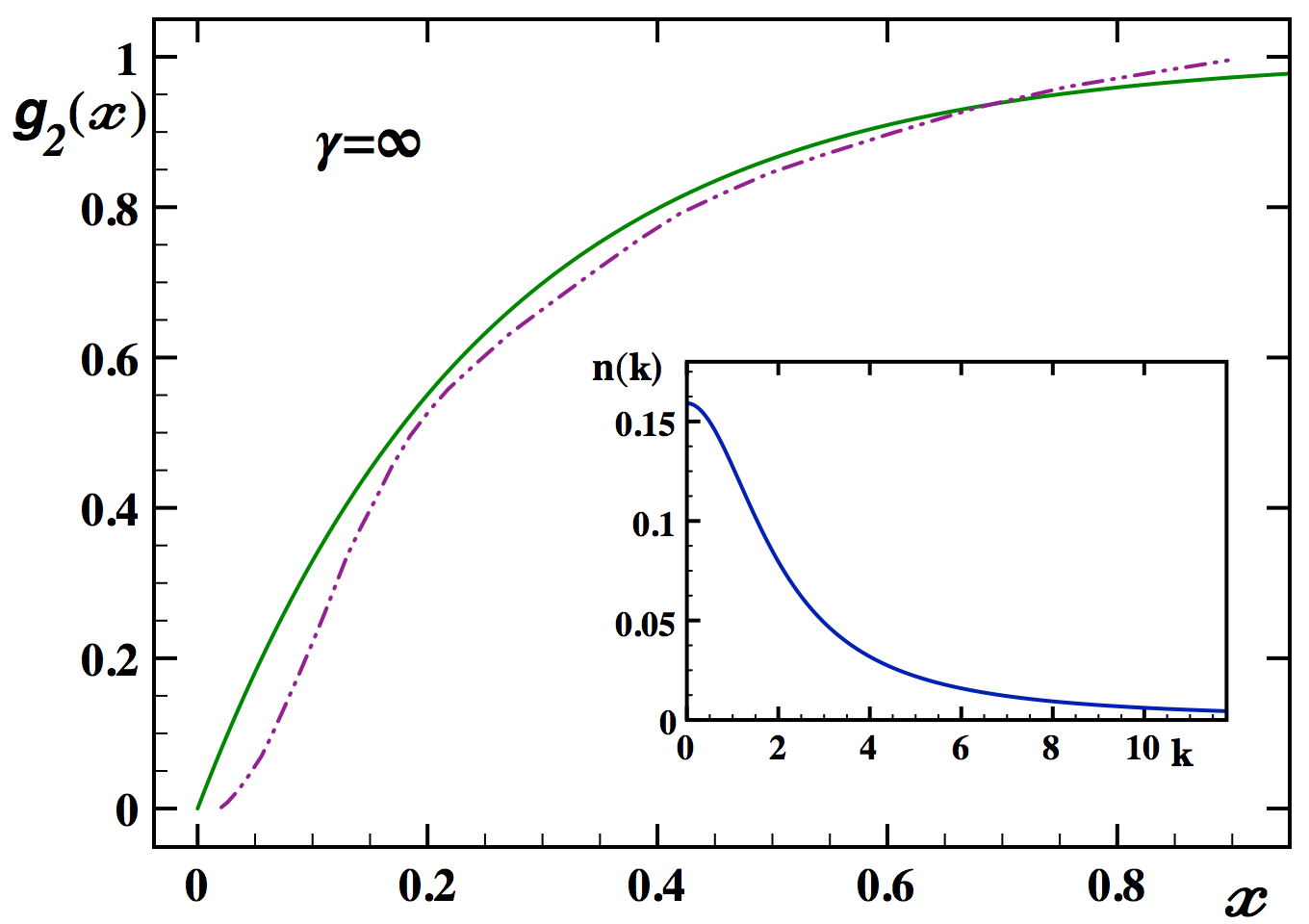
Figure 2: Quench to the TG regime ($\gamma=\infty$). Main panel: Equal time density-density correlation function. We compare GGE/saddle point (green solid) values with the large time result of a numerical solution of the dynamics of Ref. gritsev (purple dot-dot-dashed). Inset: Momentum distribution function.

We can also compute the density-density correlation function $g_{2}(x)={\langle\hat{\psi}^{\dagger}(x)\hat{\psi}^{\dagger}(0)\hat{\psi}(0)\hat{\psi}(x)\rangle}/n^{2}$ for large final $\gamma$ using the first few terms of the infinite series given in Ref. bogoliubov . In the large $\gamma$ limit the leading order for arbitrary $\rho(\lambda)$ is given by $g_{2}(x)\approx 1-\left(\int\mathrm{d}\lambda\,\rho(\lambda)e^{i\lambda x}\right)^{2}.$ Using $\rho_{s}(\lambda)$ we obtain $g_{2}(x)=1-e^{-4n|x|}$, which agrees very well with the large time result of the numerical solution of the time evolution in Ref. gritsev based on the exact overlaps (see main panel of Fig. 2). To the best of our knowledge this is one of the first demonstrations in a continuum integrable model that the GGE value of an observable agrees with its actual large time asymptotics.

Summary.—

Extending the studies of the post-quench behavior of many-body systems to a non-quadratic continuum model, we investigated the large time behavior of the Lieb–Liniger model after an interaction quench using analytic techniques by combining the Generalized Gibbs Ensemble and Bethe Ansatz integrability of the model and its lattice discretization. We pointed out the divergence of local charges in the initial state that prevents the naive application of the GGE methodology. We expect this to be a generic phenomenon for interaction quenches in continuum models which deserves further study. For a non-interacting initial state and arbitrary final interactions, we evaluated local correlations and found deviations from the thermal predictions. These are experimentally accessible through the measurement of the photoassociation rate ($g_{2}$) and the inelastic three-body loss ($g_{3}$) in cold atom experiments. We computed two-point correlation functions exactly for quenches to the femionized Tonks–Girardeau regime and found excellent agreement with a recent numerical simulation of the time evolution.

Note added.—

During the completion of the manuscript two preprints appeared XXZ which considered the truncated GGE in the BA solvable XXZ spin chain.

Supplementary Material for EPAPS
Interaction quenches in the Lieb–Liniger model

I Local conserved charges in the $q$-boson hopping model

Integrals of motion of the $q$-boson hopping model can be constructed using the Quantum Inverse Scattering Method. The $L$-operator for the model is given by

$$L_{j}(\lambda)=\left(\begin{array}[]{cc}e^{\lambda}&\chi B_{j}^{\dagger}\\ \chi B_{j}&e^{-\lambda}\end{array}\right)\,,$$ (S1)

where $\chi=\sqrt{1-q^{-2}}=\sqrt{1-e^{-2\kappa}}.$ The monodromy matrix $T(\lambda)$ is defined as a matrix product of the $L$-operators over all the lattice sites

$$T(\lambda)=L_{M}(\lambda)L_{M-1}(\lambda)\cdots L_{1}(\lambda)\,,$$ (S2)

and the transfer matrix $\tau(\lambda)$ is given by the trace over the matrix space of the monodromy matrix

$$\tau(\lambda)=\mathrm{Tr}\,T(\lambda)\,.$$ (S3)

For any $\lambda$ and $\mu$ the transfer matrices commute: $[\tau(\lambda),\tau(\mu)]=0$, which implies that $\tau(\lambda)$ is a generating function of the conserved charges. Many different sets can be generated since any analytic function of $\tau(\lambda)$ can play the role of the generating function. We consider the set consisting of local charges that can be written in the form

$$I_{m}=\delta\sum_{j=1}^{M}\mathcal{J}^{(m)}_{j}\,,$$ (S4)

where the operators $\mathcal{J}^{(m)}_{j}$ act nontrivially in $m+1$ neighboring lattice sites only. This set is obtained by the formula

$$I_{m}=\left.\frac{1}{(2m)!}\frac{d^{2m}}{d\zeta^{2m}}\ln\left[\zeta^{M}\tau(\zeta)\right]\right|_{\zeta\to 0}\,,\qquad m=1,2,3,\ldots\,.$$ (S5)

where we introduced the variable $\zeta=e^{\lambda}$. The local operators $\mathcal{J}^{(1)}(n),$ $\mathcal{J}^{(2)}(n)$ and $\mathcal{J}^{(3)}(n)$ are

$$\mathcal{J}^{(1)}(n)=\frac{1}{\delta}\chi^{2}B^{\dagger}_{j}B_{j+1}\,,$$ (S6)

$$\mathcal{J}^{(2)}(n)=\frac{1}{\delta}\chi^{2}\left(1-\frac{\chi^{2}}{2}\right)\left(B^{\dagger}_{j}B_{j+2}-\frac{\chi^{2}}{2-\chi^{2}}B_{j}^{\dagger}B_{j}^{\dagger}B_{j+1}B_{j+1}-\chi^{2}B_{j}^{\dagger}B_{j+1}^{\dagger}B_{j+1}B_{j+2}\right)\,,$$ (S7)

and

$$\mathcal{J}^{(3)}(n)=\frac{1}{\delta}\chi^{2}\left(1-\chi^{2}+\frac{\chi^{4}}{3}\right)\left(\vphantom{\frac{\chi^{4}}{3}}B^{\dagger}_{j}B_{j+3}-\chi^{2}B^{\dagger}_{j}B^{\dagger}_{j}B_{j+1}B_{j+2}-\chi^{2}B^{\dagger}_{j}B^{\dagger}_{j+1}B_{j+1}B_{j+3}\right.\\ -\chi^{2}B^{\dagger}_{j}B^{\dagger}_{j+1}B_{j+2}B_{j+2}-\chi^{2}B^{\dagger}_{j}B^{\dagger}_{j+2}B_{j+2}B_{j+3}+\frac{\chi^{4}}{3-3\chi^{2}+\chi^{4}}B^{\dagger}_{j}B^{\dagger}_{j}B^{\dagger}_{j}B_{j+1}B_{j+1}B_{j+1}\\ +\chi^{4}B^{\dagger}_{j}B^{\dagger}_{j}B^{\dagger}_{j+1}B_{j+1}B_{j+1}B_{j+2}+\chi^{4}B^{\dagger}_{j}B^{\dagger}_{j+1}B^{\dagger}_{j+1}B_{j+1}B_{j+2}B_{j+2}\\ +\left.\chi^{4}B^{\dagger}_{j}B^{\dagger}_{j+1}B^{\dagger}_{j+2}B_{j+1}B_{j+2}B_{j+3}\vphantom{\frac{\chi^{4}}{3}}\right)\,.$$ (S8)

The integrals $I_{m}$ are not Hermitian operators. Using the involution $[\tau(\zeta)]^{\dagger}=\tau(\zeta^{-1})$ it can be shown that $[I^{\dagger}_{m},I_{n}]=0$ for any $m,n$. As the number operator $N=\sum_{j}N_{j}=\sum_{j}b_{j}^{\dagger}b_{j},$ is non-polynomial in the $B^{(\dagger)}_{j}$ operators while the charges $I_{m}$ are, it cannot be expressed as a finite linear combination of the $I_{m}.$ However, $N$ commutes with any monomial containing an equal number of the creation and annihilation operators thus $[N,I_{m}]=0.$ It is convenient to use the notation $N\equiv I_{0}.$ The Hamiltonian (5) can then be written as

$$H_{q}=-\frac{1}{\chi^{2}\delta^{2}}(I_{1}+I_{-1}-2\chi^{2}I_{0})\,.$$ (S9)

II Expectation values of the charges in the initial state

We need to evaluate the expectation values of local charges $I_{m}$ in a state which transforms into the continuum BEC-state in the limit (7). We pick here the state

$$|\text{BEC}\rangle_{N}=\frac{1}{\sqrt{N!}}\left(\frac{1}{\sqrt{M}}\sum_{i}b^{\dagger}_{i}\right)^{N}|0\rangle\,,$$ (S10)

since it has the nice property (established by commuting annihilation operators one by one)

$$b^{\alpha}_{j}|\text{BEC}\rangle_{N}=\sqrt{\frac{N}{M}}\cdots\sqrt{\frac{N-\alpha+1}{M}}|\text{BEC}\rangle_{N-\alpha}\approx\nu^{\alpha/2}|\text{BEC}\rangle_{N-\alpha}\,,$$ (S11)

where the approximate relation is valid in the thermodynamic limit (TDL) when we are interested in $\alpha$ that does not scale proportionally to the system size. Note that as long as we are interested in evaluation of expectation values of normal ordered operators over BEC state in the TDL, one can also use the coherent state form of the BEC

$$|\text{BEC},c\rangle=\prod_{j}e^{-\nu/2+\sqrt{\nu}b^{\dagger}_{j}}|0\rangle\,,$$ (S12)

which has the same matrix elements as state (S11).

In what follows, we compute expectation values of the local charges by computing first the building blocks, on-site monomials, based on expanding $B^{(\dagger)}_{i}$ in terms of $b^{(\dagger)}_{i}$ and normal ordering. For most of the matrix elements we can only derive expansions in powers of $\kappa$ (but not making any assumptions about $\nu$). We will start from

$$B_{j}=b_{j}\sqrt{\frac{[N+1]_{q}}{N+1}}\approx b_{j}\left(1-\frac{\kappa}{2}N_{j}+\frac{\kappa^{2}}{24}N_{j}(5N_{j}+4)+\dots\right)=b_{j}-\frac{\kappa}{2}b_{j}^{\dagger}b_{j}b_{j}+\frac{\kappa^{2}}{24}(5b_{j}^{\dagger}b_{j}^{\dagger}b_{j}b_{j}b_{j}+9b_{j}^{\dagger}b_{j}b_{j})+\dots\,.$$ (S13)

The evaluation of its expectation value in the state (S12) leads to

$$\langle\text{BEC},c|B_{j}|\text{BEC},c\rangle=\sqrt{\nu}-\frac{1}{2}\kappa\nu^{3/2}+\frac{\kappa^{2}}{24}\left(9\nu^{3/2}+5\nu^{5/2}\right)+\dots\,.$$ (S14)

In a similar way we obtain

$$\langle\text{BEC}|B_{j}^{\dagger}B_{j}|\text{BEC}\rangle=\nu-\kappa\nu^{2}+\kappa^{2}\nu^{2}-\frac{2}{3}\nu^{2}\kappa^{3}+\frac{2}{3}\nu^{3}\kappa^{2}+\dots\,.$$ (S15)

We note that for this combination a closed form expression exists, $\langle\text{BEC}|B_{j}^{\dagger}B_{j}|\text{BEC}\rangle=(1-e^{-\left(1-q^{-2}\right)\nu})/(1-q^{-2}).$ These and similar on-site matrix elements are the only type needed to systematically evaluate the expectation values of any polynomial of $B^{(\dagger)}$ operators acting on different sites over the BEC. Indeed, due to the factorization of the wave function on different sites in the coherent state representation (S12) one can treat different sites separately.

Let us now use these matrix elements to evaluate the first $\rho_{m},$ $m=1,\dots,6.$ From Eqs. (S6,S7) and from the definition (8) we have

$$\rho_{1}=\frac{1}{M}\sum_{j}\langle B^{\dagger}_{j}B_{j+1}\rangle\,,\quad\rho_{2}=\frac{1}{M}\sum_{j}\left\langle B^{\dagger}_{j}B_{j+2}-\frac{\chi^{2}}{2-\chi^{2}}B_{j}^{\dagger}B_{j}^{\dagger}B_{j+1}B_{j+1}-\chi^{2}B_{j}^{\dagger}B_{j+1}^{\dagger}B_{j+1}B_{j+2}\right\rangle\,,\;\text{etc.}$$ (S16)

Due to translational invariance we need to evaluate the expectation value only for a single value of $j.$ We find

$$\rho_{1} =\nu-\frac{1}{2}\gamma\nu^{3}+\frac{3}{16}\gamma^{2}\nu^{4}+\left(\frac{1}{6}\gamma^{2}-\frac{7}{192}\gamma^{3}\right)\nu^{5}-\frac{11}{96}\gamma^{3}\nu^{6}+\dots\,,$$ (S17a)

$$\rho_{2} =\nu-2\gamma\nu^{3}+\frac{15}{16}\gamma^{2}\nu^{4}+\left(\frac{5}{3}\gamma^{2}-\frac{55}{192}\gamma^{3}\right)\nu^{5}+\left(-\frac{51}{32}\gamma^{3}+\frac{1}{16}\gamma^{4}\right)\nu^{6}+\dots\,,$$ (S17b)

$$\rho_{3} =\nu-\frac{9}{2}\gamma\nu^{3}+\frac{43}{16}\gamma^{2}\nu^{4}+\left(\frac{15}{2}\gamma^{2}-\frac{73}{64}\gamma^{3}\right)\nu^{5}+\left(-\frac{859}{96}\gamma^{3}+\frac{73}{192}\gamma^{4}\right)\nu^{6}+\dots\,,$$ (S17c)

$$\rho_{4} =\nu-8\gamma\nu^{3}+\frac{95}{16}\gamma^{2}\nu^{4}+\left(\frac{68}{3}\gamma^{2}-\frac{619}{192}\gamma^{3}\right)\nu^{5}+\left(-\frac{3137}{96}\gamma^{3}+\frac{269}{192}\gamma^{4}\right)\nu^{6}+\dots\,,$$ (S17d)

$$\rho_{5} =\nu-\frac{25}{2}\gamma\nu^{3}+\frac{179}{16}\gamma^{2}\nu^{4}+\left(\frac{325}{6}\gamma^{2}-\frac{1423}{192}\gamma^{3}\right)\nu^{5}+\left(-\frac{2953}{32}\gamma^{3}+\frac{379}{96}\gamma^{4}\right)\nu^{6}+\dots\,,$$ (S17e)

$$\rho_{6} =\nu-18\gamma\nu^{3}+\frac{303}{16}\gamma^{2}\nu^{4}+\left(111\gamma^{2}-\frac{949}{64}\gamma^{3}\right)\nu^{5}+\left(-\frac{21049}{96}\gamma^{3}+\frac{299}{32}\gamma^{4}\right)\nu^{6}+\dots\,,$$ (S17f)

where we use $\nu$ as small parameter by the relation

$$\kappa=\gamma\nu/2\,.$$ (S18)

Naively, combining various $\rho_{m}$ and taking the limit one can obtain moments of the $\rho_{\text{LL}}(\lambda)$ density, i.e. the expectation values of the charges $\hat{Q}_{m}$ of the LL model. However, this must be done with care. First, the limits of integration are strictly speaking not $\pm\infty$, but $\pm\pi/\delta,$ which matters if the LL moments are divergent (as expected). Second, the scaling limit (7), Eq.  (S18) as well as the relations $\lambda=p/\delta$ and $\rho_{\text{LL}}(\lambda)=\rho_{q}(\delta\,\lambda)$ may have higher order corrections which would mix the orders.

In spite of the problems mentioned above, the energy can be obtained if the $\rho_{\text{LL}}(\lambda)$ has at most a $\lambda^{-4}$ tail:

$$-\frac{1}{4}(\rho_{1}+\rho_{-1}-2\rho_{0})=\int_{-\pi}^{\pi}\mathrm{d}p\,(p^{2}-\frac{1}{6}p^{4}+\dots)\rho_{q}(p)=\int_{-\pi/\delta+\dots}^{\pi/\delta+\dots}\mathrm{d}\lambda(\delta+\dots)(\delta^{2}\lambda^{2}-\frac{1}{6}\lambda^{4}\delta^{4}+\dots)(\rho_{\text{LL}}(\lambda)+\dots)\,,$$ (S19)

where the dots stand for higher order terms in $\delta$. The first parenthesis comes from the unknown higher order terms of the relation $p=\delta\cdot\lambda+\dots$, this also generates terms in the middle parenthesis. Now let us make the assumption that this relation, as well as the relation between $\rho(p)$ and $\rho_{\text{LL}}(\lambda)$ does not have higher powers of $\lambda$. Under this assumption each power $\lambda^{2n}$ comes with at least $\delta^{2n+1}$ in the integrand which implies that although the integrals of higher powers seem to diverge, with the $\delta$-powers in their coefficients all of them scale as $\delta^{4}$, while the quadratic term scales as $\delta^{3}$. Thus it is safe to take the $\delta\to 0$ limit after dividing by $\delta^{3}$ and we are left with

$$-\frac{1}{2\delta^{3}}(\rho_{1}-\rho_{0})\to\int_{-\infty}^{\infty}\mathrm{d}\lambda\,\rho_{\text{LL}}(\lambda)\lambda^{2}\,.$$ (S20)

Since $\lim_{\delta\to 0}\left[-\frac{1}{2\delta^{3}}(\rho_{1}-\rho_{0})\right]=n^{3}\gamma$, the energy density is correctly reproduced, as expected.

In a similar fashion, one can formulate a condition on whether the $2n$-th moment of the $\rho_{\text{LL}}(\lambda)$ distribution is divergent. For this one again needs to pick the right combination of $\rho_{m}$ with $m\leq n.$ In particular, $Q_{4}$ is divergent if

$$\rho_{2}+\rho_{-2}-2\rho_{0}-4(\rho_{1}+\rho_{-1}-2\rho_{0})\propto\delta^{4}\,,$$ (S21)

as opposed to $\propto\delta^{5}$. From the expansion in Eqs. (S17) we find

$$\rho_{2}-\rho_{0}-4(\rho_{1}-\rho_{0})=\frac{3}{\gamma^{2}}\kappa^{4}+\dots\,,$$ (S22)

thus $\int\mathrm{d}\lambda\rho_{\text{LL}}(\lambda)\lambda^{4}={\langle Q_{4}\rangle}/L$ is divergent.

III Pattern for expectation values in the BEC state

Based on the Taylor expansions in Eqs. (S17) one can find a pattern for the coefficients of the different orders. They turn out to be low order polynomials in $m$:

$$\rho_{m}=\nu-\frac{m^{2}}{2}\gamma\nu^{3}+\frac{m^{3}+2m-\frac{3}{4}}{12}\gamma^{2}\nu^{4}+\left(\frac{m^{2}(m^{2}+1)}{12}\gamma^{2}-\frac{m^{4}+4m^{2}-3m+\frac{3}{2}}{96}\gamma^{3}\right)\nu^{5}\\ +\left(-\frac{m^{5}+5m^{3}-\frac{5}{2}m^{2}+\frac{2}{3}m+\frac{5}{12}}{40}\gamma^{3}+\frac{m^{5}+\frac{20}{3}m^{3}-\frac{15}{2}m^{2}+\frac{29}{6}m-5}{960}\gamma^{4}\right)\nu^{6}+\mathcal{O}(\nu^{7})\,.$$ (S23)

The reasonably simple rational coefficients and their structure provide strong evidence that the polynomial dependence on $m$ is correct. The order of the coefficient polynomial of $\nu^{k}$ is $k-1$ and, interestingly, the subleading orders ($m^{k-2}$) are always missing. As we will show now, the first property is necessary in order to have a finite scaling limit of the $\rho(p)$ function, i.e. a finite $\rho_{\text{LL}}(\lambda)$.

The $\rho(p)$ distribution function is the Fourier sum of the $\rho_{m}$. It is clear that the scaling limit and this Fourier transformation do not commute: if we take the limit before computing the sum we get $\rho_{m}\equiv 0$. For the computation of the Fourier sum order by order in $\nu$ one needs to calculate the building blocks

$$\sum_{m=-\infty}^{\infty}m^{2l}\cos(mp) =0\,,$$ (S24)

$$\sum_{m=-\infty}^{\infty}m^{2l-1}\cos(mp) =\frac{\sum_{j=0}^{l-1}c_{j}\cos(jp)}{\sin^{2l}\left(\frac{p}{2}\right)}\longrightarrow\frac{2^{2l}\sum_{j=0}^{l-1}c_{j}}{\delta^{2l}\lambda^{2l}}\,,$$ (S25)

where the $c_{j}$ are real numbers. This must be multiplied by $\delta^{2l}$ to be neither divergent nor zero. Thus the fact that in Eq. (S23) the highest power of $m$ in the coefficient of $\nu^{k}$ is $k-1$ implies that $\rho_{\text{LL}}(\lambda)$ is finite. Moreover, only the highest powers of $m$ in the coefficient polynomials of the even orders of $\nu$ contributes. This is important, because we know the relation $\kappa=\gamma\nu/2$ only to leading order. Adding potential sub-leading terms, $\kappa=\gamma\nu/2+a_{1}\nu^{2}+a_{2}\nu^{3}+\dots$, generates terms in each order of $\nu$ which however have a sub-leading $m$-dependence, thus they will do not affect the result in the continuum limit.

Taking the Fourier sum we obtain

$$2\pi\rho(p)=\rho_{0}+2\sum_{m=1}^{\infty}\rho_{m}\cos(mp)=\nu+2\sum_{m=1}^{\infty}\left(\frac{1}{12}\gamma^{2}\nu^{4}m^{3}+\frac{\gamma^{3}(\gamma-24)}{960}\nu^{6}m^{5}\right)+\text{[``subleading terms'']}+\dots{\\ }=\nu+2\left(\nu^{4}\frac{\gamma^{2}}{12}\,\frac{2+\cos(p)}{8\sin^{4}(p/2)}-\nu^{6}\frac{\gamma^{3}(\gamma-24)}{960}\,\frac{33+26\cos(p)+\cos(2p)}{32\sin^{6}(p/2)}+\dots\right)\,.$$ (S26)

Taking the continuum limit (7) together with $p=\delta\lambda$ we find

$$\rho_{\text{LL}}(\lambda)=\frac{n^{4}\gamma^{2}}{\lambda^{4}}-\frac{n^{6}\gamma^{3}(\gamma-24)}{4\lambda^{6}}+\dots\,.$$ (S27)

We see that the expansion of the Fourier modes $\rho_{m}$ in terms of $\delta$ or $\nu$ is equivalent to a large momentum expansion of the LL density of roots $\rho_{\text{LL}}(\lambda)$. We did find the expected $\lambda^{-4}$ tail together with the subleading $\lambda^{-6}$ tail.

Observe that going to higher charges and to higher powers in $\nu$ go side by side: if one only expands the $\rho_{m}$ up to a fixed order in $\nu$ then one does not gain anything from considering many more charges because the polynomial pattern found from the lower ones already determines them. Conversely, having only a few charges does not allow one to determine the high order polynomial coefficients of the higher orders of $\nu$.

A key step in all the above is the rescaling of momenta, $\lambda=p/\delta$. This is how lower orders of $\nu$ may eventually disappear and arbitrary high powers of $\nu$ may survive in the limit. Consequently, the large momentum expansion structure can be heuristically understood by realizing that we need to resolve the vicinity of $p=0$ very well, because this region will be blown up to be the entire domain in $\lambda$. Thus it is not very surprising that many Fourier modes are necessary and one needs to know them very precisely. Any truncation or approximation affects the small $\lambda$ region, so perturbatively we approach from large $\lambda$.

IV Padé–Fourier approximation

Let us consider the truncated Fourier sum,

$$\rho^{[l]}(p)=\rho_{0}+2\sum_{m=1}^{l}\rho_{m}\cos(mp)=\left(\frac{\rho_{0}}{2}+\sum_{m=1}^{l}\rho_{m}e^{imp}\right)+\{p\to-p\}=\left(\frac{\rho_{0}}{2}+\sum_{m=1}^{l}\rho_{m}z^{m}\right)+\{z\to 1/z\}\,,$$ (S28)

where we introduced $z=e^{ip}$. The parenthesis is a truncated Taylor expansion to which we apply the Hermite–Padé approximation technique: we find a rational function of $z$ such that the first $l$ terms in its Tayor expansion matches our truncated expansion. The $(n,m)$-type Padé-approximant is a ratio of an $n$th order and an $m$th order polynomial ($n+m=l$). We reintroduce the variable $p$ in the approximants and then we take the continuum limit. The $(2,2)$, $(3,2)$, $(2,3)$, $(4,2)$ and $(2,4)$ Padé-approximants all give the same result, Eq. (10):

$$\rho^{(1)}_{\text{LL}}(\lambda)=\frac{1}{2\pi}\frac{\gamma^{2}}{(\lambda/n)^{4}+\gamma(\gamma/4-2)(\lambda/n)^{2}+\gamma^{2}}\,.$$ (S29)

Comparing with Eq. (S27) this has the correct $\lambda^{-4}$ tail but not the $\lambda^{-6}$ one. The latter is reproduced by the Padé-approximant of type $(3,3)$:

$$\rho^{(2)}_{\text{LL}}(\lambda)=\frac{1}{2\pi}\frac{4\gamma^{2}\left(\bar{\lambda}^{2}+\gamma(\gamma+2)\right)}{(4\bar{\lambda}^{2}+\gamma^{2})\left(\bar{\lambda}^{4}+(\gamma-4)\gamma\,\bar{\lambda}^{2}+4\gamma^{2}\right)}\,,$$ (S30)

where $\bar{\lambda}=\lambda/n$. The $\gamma\to\infty$ limit of both $\rho^{(1)}(\lambda)$ and $\rho^{(2)}(\lambda)$ is given by Eq. (11).

References

- (1) I. Bloch, J. Dalibard, and W. Zwerger, Rev. Mod. Phys. 80, 885 (2008).
- (2) M. Greiner, O. Mandel, T. W. Hänsch, and I. Bloch, Nature 419 51 (2002).
- (3) T. Kinoshita, T. Wenger, and D. S. Weiss, Nature 440, 900 (2006).
- (4) S. Hofferberth, I. Lesanovsky, B. Fischer, T. Schumm, and J. Schmiedmayer, Nature 449, 324 (2007).
- (5) E. Haller, M. Gustavsson, M.J. Mark, J.G. Danzl, R. Hart, G. Pupillo, and H.-C. Nägerl, Science 325, 1224 (2009).
- (6) S. Trotzky Y.-A. Chen, A. Flesch, I. P. McCulloch, U. Schollwöck, J. Eisert, and I. Bloch, Nature Phys. 8, 325 (2012).
- (7) M. Cheneau, P. Barmettler, D. Poletti, M. Endres, P. Schauss, T. Fukuhara, C. Gross, I. Bloch, C. Kollath, and S. Kuhr, Nature 481, 484 (2012).
- (8) M. Gring, M. Kuhnert, T. Langen, T. Kitagawa, B. Rauer, M. Schreitl, I. Mazets, D. A. Smith, E. Demler, and J. Schmiedmayer, Science 337, 1318 (2012).
- (9) U. Schneider, L. Hackermüller, J.P. Ronzheimer, S. Will, S. Braun, T. Best, I. Bloch, E. Demler, S. Mandt, D. Rasch, and A. Rosch, Nature Phys. 8, 213 (2012).
- (10) J.P. Ronzheimer, M. Schreiber, S. Braun, S.S. Hodgman, S. Langer, I.P. McCulloch, F. Heidrich-Meisner, I. Bloch, and U. Schneider, Phys. Rev. Lett. 110, 205301 (2013).
- (11) M. Rigol, V. Dunjko, and M. Olshanii, Nature 452, 854 (2008); J. Dziarmaga, Adv. Phys. 59, 1063 (2010); A. Polkovnikov, K. Sengupta, A. Silva, and M. Vengalattore, Rev. Mod. Phys. 83, 863 (2011).
- (12) H. Tasaki, Phys. Rev. Lett. 80, 1373 (1998); S. Goldstein, J.L. Lebowitz, R. Tumulka, and N. Zanghì, Phys. Rev. Lett. 96, 050403 (2006); S. Popescu, A.J.Short, and A. Winter, Nat. Phys. 2, 754 (2007); P. Reimann, Phys. Rev. Lett. 99, 160404 (2007); Phys. Rev. Lett. 101, 190403 (2008); N. Linden, S. Popescu, A.J. Short, and A. Winter, Phys. Rev. E 79, 061103 (2009); A.J. Short, New J. Phys. 13, 053009 (2011); A.J. Short, T.C. Farrelly, New J. Phys. 14, 013063 (2012).
- (13) P. Calabrese and J. Cardy, Phys. Rev. Lett. 96, 136801 (2006), J. Stat. Mech. P06008 (2007).
- (14) M. Eckstein, M. Kollar, and P. Werner, Phys. Rev. Lett. 103, 056403 (2009); A. Faribault, P. Calabrese, and J.-S. Caux, J. Stat. Mech. P03018 (2009); G. Biroli, C. Kollath, and A.M. Läuchli, Phys. Rev. Lett. 105, 250401 (2010); M.C. Bañuls, J.I. Cirac, and M.B. Hastings, Phys. Rev. Lett. 106, 050405 (2011); C. Gogolin, M.P. Müller, and J. Eisert, Phys. Rev. Lett. 106, 040401 (2011); S. Sotiriadis, D. Fioretto, and G. Mussardo, J. Stat. Mech. P02017 (2012); G. P. Brandino, A. De Luca, R. M. Konik, and G. Mussardo, Phys. Rev. B 85, 214435 (2012); J. Marino and A. Silva, Phys. Rev. B 86, 060408 (2012); C. Gramsch and M. Rigol, Phys. Rev. A 86, 053615 (2012);
- (15) H. Buljan, R. Pezer, and T. Gasenzer, Phys. Rev. Lett. 100, 080406 (2008); D. Muth, B. Schmidt, and M. Fleischhauer, New Journal of Physics 12, 083065 (2010); D. Muth and M. Fleischhauer, Phys. Rev. Lett. 105, 150403 (2010); D. Iyer and N. Andrei, Phys. Rev. Lett. 109, 115304 (2012); arXiv:1304.0506; J.-S. Caux and R. M. Konik, Phys. Rev. Lett. 109, 175301 (2012); J. Mossel and J.-S. Caux, New J. Phys. 14 075006 (2012); M. Collura, S. Sotiriadis, and P. Calabrese, arxiv:1303.3795.
- (16) D. Rossini, A. Silva, G. Mussardo, and G. Santoro, Phys. Rev. Lett. 102, 127204 (2009); D. Rossini, S. Suzuki, G. Mussardo, G. E. Santoro, and A. Silva, Phys. Rev. B 82, 144302 (2010); P. Calabrese, F.H.L. Essler, and M. Fagotti, Phys. Rev. Lett. 106, 227203 (2011); J. Stat. Mech. (2012) P07016; J. Stat. Mech. (2012) P07022; L. Foini, L.F. Cugliandolo, and A. Gambassi, Phys. Rev. B 84, 212404 (2011); J. Stat. Mech. (2012) P09011. F.H.L. Essler, S. Evangelisti, and M. Fagotti, Phys. Rev. Lett. 109, 247206 (2012); D. Schuricht and F. H. L. Essler, J. Stat. Mech. P04017 (2012); M. Heyl, A. Polkovnikov and S. Kehrein, Phys. Rev. Lett. 110, 135704 (2013).
- (17) M.A. Cazalilla, Phys. Rev. Lett. 97, 156403 (2006); A. Iucci and M.A. Cazalilla, Phys. Rev. A 80, 063619 (2009) C. Karrasch, J. Rentrop, D. Schuricht, and V. Meden, Phys. Rev. Lett. 109, 126406 (2012); J. Rentrop, D. Schuricht, and V. Meden, New J. Phys. 14, 075001 (2012);
- (18) M. Rigol, V. Dunjko, V. Yurovsky, and M. Olshanii, Phys. Rev. Lett. 98, 050405 (2007).
- (19) S.R. Manmana, S. Wessel, R.M. Noack, and A. Muramatsu, Phys. Rev. Lett. 98, 210405 (2007); D. M. Gangardt and M. Pustilnik, Phys. Rev. A 77, 041604(R) (2008); A. Iucci and M.A. Cazalilla, New J. Phys. 12, 055019 (2010); A.C. Cassidy, C.W. Clark, and M. Rigol, Phys. Rev. Lett. 106, 140405 (2011); M. Rigol and M. Fitzpatrick, Phys. Rev. A 84, 033640 (2011); M. A. Cazalilla, A. Iucci, and M.-C. Chung, Phys. Rev. E 85, 011133 (2012).
- (20) M. Eckstein and M. Kollar, Phys. Rev. Lett. 100, 120404 (2007); M. Kollar and M. Eckstein, Phys. Rev. A 78, 013626 (2008); M. Kollar, F.A. Wolf, and M. Eckstein, Phys. Rev. B 84, 054304 (2011); E. Demler and A. M. Tsvelik, Phys. Rev. B 86, 115448 (2012); V. Gurarie, J. Stat. Mech. P02014 (2013); M. Fagotti, Phys. Rev. B 87, 165106 (2013); G. Mussardo, arxiv:1304.7599.
- (21) D. Fioretto and G. Mussardo, New J. Phys. 12 055015, (2010).
- (22) J. Mossel and J.-S. Caux, J. Phys. A 45, 255001 (2012).
- (23) T. Barthel and U. Schollwöck, Phys. Rev. Lett. 100, 100601 (2008); M. Cramer, C. M. Dawson, J. Eisert, and T. J. Osborne, Phys. Rev. Lett. 100, 030602 (2008); M. Cramer and J. Eisert, New J. Phys. 12, 055020 (2010).
- (24) J.-S. Caux and F.H.L. Essler, arxiv:1301.3806.
- (25) M. Fagotti and F.H.L. Essler, arxiv:1302.6944.
- (26) E.H. Lieb and W. Liniger, Phys. Rev. 130, 1605 (1963); E.H. Lieb, Phys. Rev. 130, 1616 (1963).
- (27) B. Sutherland, Beautiful Models , World Scientific (2004).
- (28) M. Olshanii, Phys. Rev. Lett. 81, 938 (1998);
- (29) V.E. Korepin, N.M. Bogoliubov, and A.G. Izergin, Quantum Inverse Scattering Method and Correlation Functions (Cambridge University Press, Cambridge, 1993).
- (30) C.N. Yang and C.P. Yang, J. Math. Phys. 10, 1115 (1969).
- (31) B. Davies, Physica A 167, 433 (1990); B. Davies and V.E. Korepin, arXiv:1109.6604.
- (32) J. Mossel, Ph.D. thesis, University of Amsterdam (2012).
- (33) N.M. Bogoliubov, R.K. Bullough, and G.D. Pang, Phys. Rev. B 47, 11495 (1993); N.M. Bogoliubov, A.G. Izergin, and N.A. Kitanine, Nucl. Phys. B 516, 501 (1998).
- (34) V.V. Cheianov, H. Smith, and M.B. Zvonarev, J. Stat. Mech. P08015 (2006).
- (35) See Supplemental Material
- (36) M. Kormos, G. Mussardo, and A. Trombettoni, Phys. Rev. Lett. 103, 210404 (2009); Phys. Rev. A 81, 043606 (2010); M. Kormos, Y.-Z. Chou, and A. Imambekov, Phys. Rev. Lett. 107, 230405 (2011); E. Haller, M. Rabie, M.J. Mark, J.G. Danzl, R. Hart, K. Lauber, G. Pupillo, and H.-C. Nägerl, Phys. Rev. Lett. 107, 230404 (2011); B. Pozsgay, J. Stat. Mech. (2011) P01011.
- (37) V. Gritsev, T. Rostunov, and E. Demler, J. Stat. Mech. (2010) P05012.
- (38) A. Imambekov, I.E. Mazets, D.S. Petrov, V. Gritsev, S. Manz, S.Hofferberth, T. Schumm, E. Demler, and J. Schmiedmayer, Phys. Rev. A 80, 033604 (2009);
- (39) J. De Nardis, B. Wouters, M. Brockmann, and J.-S. Caux, in preparation
- (40) N. M. Bogoliubov and V. E. Korepin, Theor. Math. Phys. 60, 808 (1984).
- (41) B. Pozsgay, arxiv:1304.5374; M. Fagotti and F.H.L. Essler , arxiv:1305.0468.