Holographic Rényi Entropies at Finite Coupling

Abstract

We compute Rényi entropies for a spherical entangling surface in four-dimensional ${\cal{N}}=4$ super-Yang-Mills at strong coupling using the AdS/CFT correspondence. Incorporating the effects of the leading $\alpha^{\prime}$ corrections to the low energy effective action of type IIB string theory, we calculate the leading corrections in inverse powers of the ’t Hooft coupling (and the number of colours). The results are compared with known weak coupling calculations. Setting the order of the Rényi entropy $q$ to one, it reduces to the entanglement entropy and the strong and weak coupling results match without any corrections, as expected. In the limit of $q\rightarrow 0$, the relation between the strong and weak coupling entropies is connected to the known corrections for the thermal free energy in flat space. We also compute the correction to the scaling dimension of twist operators.

1 Introduction

Entanglement is emerging as a fundamental phenomena in a wide variety of areas ranging from quantum information and condensed matter physics, e.g., wenx ; cardy0 to quantum gravity and string theory, e.g., sorkin ; suss ; rt1 . A useful probe for entanglement in quantum systems is the entanglement entropy (EE). Given a subsystem $A$, one constructs the reduced density matrix $\rho_{A}$ by tracing over the degrees of freedom in the complement to $A$ for some global state or density matrix describing the full system. Then, the EE is simply defined as the von Neumann entropy of $\rho_{\textrm{\tiny A}}$: $S_{\textrm{\tiny EE}}\equiv-$tr$(\rho_{\textrm{\tiny A}}\log\rho_{\textrm{\tiny A}})$. This can be extended to a more general family of entanglement measures known as entanglement Rényi entropies (ERE) renyi0 ; renyi1 . These are defined as

$$S_{q}=\frac{1}{1-q}\log{\rm tr}(\rho_{\textrm{\tiny A}}^{\,q})\,,$$ (1)

where $q$ is a real positive number called the order of the ERE. By design given $S_{q}$ for a particular system, one can recover the usual EE with the limit: $S_{\textrm{\tiny EE}}=\lim_{q\to 1}S_{q}$. However, the full family of ERE clearly provides much more information about the density matrix, i.e., in principle, one can determine the full spectrum of eigenvalues of $\rho_{\textrm{\tiny A}}$ calab8 .

Generally, it is also easier to calculate ERE than EE since the former avoids the difficulty of calculating the logarithm of the density matrix. However, in the context of quantum field theory, as we consider in this paper, the calculation of ERE generally remains a challenging task. In two-dimensional conformal field theory (CFT), there is a universal result for the ERE of an interval of length $\ell$ cardy0 :

$$S_{q}(d=2)=\frac{c}{6}\left(1+\frac{1}{q}\right)\log(\,\ell/\delta)\,,$$ (2)

where $c$ is the central charge and $\delta$ is a short-distance regulator, in the underlying CFT. In higher dimensions, the explicit results for ERE, as well as our general understanding of these entanglement measures, are much more limited cmt . Essentially, any such results for ERE rely on the ‘replica trick,’ which requires evaluating the partition function on a $q$-fold cover of the original background geometry cardy0 ; Callan:1994py .

Recently, the AdS/CFT correspondence m1 has provided an alternative perspective on EE for (certain) strong strongly coupled gauge theories. In particular, the EE for a region in the boundary theory is calculated by evaluating the black hole entropy formula on a corresponding extremal surface in the dual bulk spacetime rt1 . At a fundamental level, this prescription suggests that EE plays an important role in the quantum structure of spacetime, e.g., mvr ; vm ; arch . An alternative approach to determine holographic EE for spherical entangling surfaces was proposed in Casini:2011kv — see also cthem — which has a number of advantages. First, while the standard prescription rt1 only applies when the bulk physics is described by Einstein gravity, the approach of Casini:2011kv can also be applied to bulk gravitational theories which include arbitrary higher curvature interactions. Further, while progress on a holographic ERE had been limited primarly to considering two-dimensional boundary CFT’s Headrick:2010zt , this alternative approach for spherical entangling surfaces is easily generalized to calculating ERE for the same surfaces in higher dimensional boundary CFT’s Hung:2011nu . Both of these features will be essential for in the following where we use the holographic construction of Casini:2011kv ; Hung:2011nu to study the ERE of four-dimensional ${\cal{N}}=4$ super-Yang-Mills (SYM) at strong coupling.

Let us briefly review the discussion of Casini:2011kv . They considered CFT’s in flat $d$ dimensional Minkowski spacetime and computed the EE for a spherical entangling surface of radius $R$. The causal domain of the region enclosed by this sphere can be mapped using a conformal transformation to a hyperbolic cylinder $R\times H^{d-1}$. The curvature scale of the hyperbolic hyperplane is given by the radius of the original sphere. Further, if the CFT began in the vacuum in flat space then, after the conformal mapping, one has a thermal ensemble in the new geometry with temperature

$$T_{0}=\frac{1}{2\pi R}\,.$$ (3)

Hence, the EE for the spherical region of the CFT is equivalent to the thermal entropy of the CFT at temperature $T_{0}$ on the hyperbolic cylinder. Further, if the theory admits an holographic dual, then, using the AdS/CFT correspondence, we can translate this thermal entropy to the horizon entropy of an appropriate black hole in the dual AdS spacetime. In fact, the latter is found to be a so-called ‘topological black hole’, i.e., an asymptotically AdS black hole for which the event horizon has the geometry $H^{d-1}$. Indeed, this calculation does not rely on having Einstein gravity in the bulk, since we simply evaluate the horizon entropy using Wald’s formula Wald in cases where there are higher curvature interactions.

As we mentioned previously, Hung:2011nu showed that the above argument can be extended to calculate holographic entanglement Rényi entropies for a spherical entangling surfaces. First we observe that in the case of interest, the trace of the power of the density matrix appearing in eq. (1) can be related to a thermal partition function with a new temperature, i.e., 

$$tr(\rho_{\textrm{\tiny A}}^{\,q})=\frac{Z(T_{0}/q)}{Z(T_{0})^{q}}\,.$$ (4)

Then using standard thermodynamic relations, the ERE can be related to the thermal free energy of the CFT on the cylinder with

$$S_{q}=\frac{q}{1-q}\frac{1}{T_{0}}(F(T_{0})-F(T_{0}/q))\,.$$ (5)

Alternatively, the ERE can be expressed in terms of the thermal entropy using,

$$S_{q}=\frac{q}{q-1}\frac{1}{T_{0}}\int_{T_{0}/q}^{T_{0}}S_{therm}(T)\ dT\,.$$ (6)

With these expressions in hand, we can evaluate the ERE in the holographic framework by determining the required thermodynamic properties of the boundary CFT on the hyperbolic cylinder by analyzing the same characteristics of the dual family of topological black holes in the bulk theory.

As we said above, the aim of the present paper is to apply these expressions to study the ERE for the most famous example of the AdS/CFT correspondence, namely, four-dimensional ${\cal{N}}=4$ $SU(N)$ super-Yang-Mills (SYM) dual to type IIB string theory on an AdS${}_{5}\times$S⁵ background. This duality is usually studied in the limit of an infinite number of colours and an infinite ’t Hooft coupling, i.e., $N\rightarrow\infty$ and $\lambda=g_{YM}^{2}N\to\infty$ (while $\lambda/N\to 0$), so that we get classical supergravity as the dual bulk theory. In this limit, we only need to interpret the holographic calculations found in Hung:2011nu to apply them to the case of ${\cal N}=4$ SYM. However, we can also begin to relax the conditions on the coupling by analyzing the effect of the leading stringy corrections to the low-energy effective action. In type IIB string theory, the leading correction to the supergravity action appears at $O(\alpha^{\prime 3})$ curv4 ; curv4a and this naturally leads to corrections of order $\lambda^{-3/2}$ in the dual SYM theory. In fact, by examining the detailed form of these higher derivative corrections in the effective action instant ; Paulos:2008tn , we can argue that they also capture the first finite $N$ corrections proportional to $\lambda^{1/2}/N^{2}$ Myers:2008yi .

Our results for the ERE will be very much analogous to holographic results for the thermal entropy of SYM in the large $N$ limit. In particular, for a thermal bath in flat space, the entropy density can be written as $s(T)=\frac{2\pi^{2}}{3}\,N^{2}\,T^{3}\,f(\lambda)$ where the function $f(\lambda)$ encodes the dependence on the ’t Hooft coupling. In the strong coupling limit, holographic calculations indicate this function takes the form Gubser:1998nz ; Pawelczyk:1998pb

$$f(\lambda\to\infty)=\frac{3}{4}+\frac{45}{32}\frac{\zeta(3)}{\lambda^{3/2}}+\cdots,$$ (7)

where the $\cdots$ indicate terms involving higher inverse powers of $\lambda$. While at weak coupling, a two-loop calculation is required to show loopy

$$f(\lambda\to 0)=1-\frac{3}{4\pi^{2}}\lambda+\cdots,$$ (8)

where now $\cdots$ indicate contributions with higher powers of $\lambda$. Of course, there is a mismatch in this two limits by a celebrated factor of $3/4$. However, the fact that the leading corrections are positive at strong coupling and negative at weak coupling suggest that $f(\lambda)$ is continuous function that interpolates smoothly between these two limits.

The rest of the paper is organized as follows: In section 2, we review the results for the ERE of a spherical entangling surface in SYM, both at weak coupling Fursaev:2012mp and strong coupling Hung:2011nu . In section 3, we will determine the effect of the leading $\alpha^{\prime 3}$ corrections in the effective action. We also analyze corrections that this interaction produces for the scaling dimension of twist operators that arise in calculations of the ERE. Section 4 presents a brief discussion of our results. Appendix A provides an alternate calculation of the corrections to the ERE induced by the leading $\alpha^{\prime 3}$ terms in the type IIB action, which gives a consistency check for our analysis in section 3.

2 ERE at weak and strong coupling

In this section, we review the two known calculations for ERE of spherical surfaces of radius $R$ in ${\cal{N}}=4$ $SU(N)$ super-Yang-Mills. The first one was obtained in the limit of zero ’t Hooft coupling, i.e., free fields. The second one, obtained via holography, gives the value of ERE at infinitely strong coupling and infinite $N$. Using the holographic dictionary, we will show how these two solutions relate to each other. While for general $q$ the ERE’s at strong and weak coupling do not agree, the hope would be that there exists some continuous function of the coupling that interpolates between the two solutions.

2.1 ERE at weak coupling

At weak coupling, ERE for spherical entangling surfaces of radius $R$ were calculated in Fursaev:2012mp . Here we are considering the free field limit of the SYM theory and so one only needs to sum the contributions for a gauge field, four complex Weyl fermions and six massless (conformally coupled) scalars, all in the adjoint representation. That computation yields, in the large $N$ limit,

$$S_{q}(R)\simeq N^{2}\left(\frac{1}{2\,q}\frac{R^{2}}{\delta^{2}}-\frac{1+q+7q^{2}+15q^{3}}{24q^{3}}\log\left(\frac{R}{\delta}\right)\right),$$ (9)

where $\delta$ is a short-distance cut-off. The first contribution is the expected area law term but the coefficient of this power law divergence is not universal. Hence, we focus on the $\log$ term, which is expected to be universal, i.e., independent of any regularization scheme. Therefore, this contribution will be the interesting one to compare with the strong coupling results.

As we will be comparing ERE for different values of $q$, it will be useful to write

$$S^{\log}_{q}(R)=-N^{2}s(q)\log\left(\frac{R}{\delta}\right),$$ (10)

where we are defining

$$s^{\text{weak}}(q)=\frac{1+q+7q^{2}+15q^{3}}{24q^{3}}.$$ (11)

Note that with $q=1$, for which the ERE reduces to the entanglement entropy, we have $s^{\text{weak}}(q=1)=1$.

2.2 ERE at strong coupling

At strong coupling, we will follow Hung:2011nu and briefly review how the holographic result is calculated. This review will also set the stage for our calculation on the corrections to the ERE in the next section.

The dual gravitational theory is simply five-dimensional Einstein gravity with negative cosmological constant, whose action is

$$I_{bulk}=\frac{1}{2\ell_{\textrm{\tiny P}}^{3}}\int d^{5}x\sqrt{-g}\left(R+\frac{12}{L^{2}}\right),$$ (12)

where we defined $\ell_{\textrm{\tiny P}}^{3}=8\pi G_{N}$. The topological black hole that satisfies the corresponding equations of motion has a metric given by

$$ds^{2}=-\left(\frac{r^{2}}{L^{2}}\left(1-\frac{\omega^{4}}{r^{4}}\right)-1\right)\frac{L^{2}}{R^{2}}dt^{2}+\frac{dr^{2}}{\frac{r^{2}}{L^{2}}\left(1-\frac{\omega^{4}}{r^{4}}\right)-1}+r^{2}d\Sigma^{2}_{3},$$ (13)

where $d\Sigma^{2}_{3}$ is the line element for $H^{3}$, the hyperbolic plane in three dimensions with unit curvature. Note that we chose to include a factor $L^{2}/R^{2}$ in $g_{tt}$ term to ensure that the curvature scale of the boundary metric is $R$. That is, the boundary CFT lives on the hyperbolic cylinder $R\times H^{3}$ with metric,

$$ds^{2}_{bndry}=-dt^{2}+R^{2}\,d\Sigma^{2}_{3}\,.$$ (14)

We always have the freedom to adjust this constant factor as is convenient since it simply corresponds to a constant rescaling of the time coordinate. The event horizon in the above metric (13) is found by setting $g_{tt}$ to zero. The latter then yields a relation between $\omega$ and the position of the event horizon $r_{h}$,

$$\omega^{4}=r_{h}^{4}-L^{2}r_{h}^{2}\,.$$ (15)

Another important aspect of this geometry is that the horizon ‘area’ is proportional to the volume of the hyperbolic plane, $V_{\Sigma_{3}}=\int d\Sigma$, which is divergent. Of course, the latter is closely related to the UV divergences appearing in the Rényi entropies Casini:2011kv ; Hung:2011nu . Hence, in order to get a finite result, one only integrates up to some maximum radius defined by the asymptotic cut-off surface in the AdS spacetime. This regulator is defined in terms of $\delta$, the short distance cut-off in the boundary theory. Then one can expand the volume $V_{\Sigma_{3}}$ in powers of $R/\delta$ and of particular interest for the present calculation, we can identify the universal log term

$$V_{\Sigma_{3},univ}=-2\pi\log\left(\frac{R}{\delta}\right).$$ (16)

In order to calculate ERE with eq. (6), we need to know both the temperature and the entropy of this solution. As usual, the temperature is defined as the Hawking temperature and the entropy is given by the horizon area, i.e., $S=\frac{2\pi A}{\ell_{\textrm{\tiny P}}^{3}}$. For the above geometry (13), we find

$$T(x) = T_{0}\left(2x-\frac{1}{x}\right)\equiv T_{1}(x),$$ (17)

$$S(x) = 2\pi V_{\Sigma_{3}}\left(\frac{L}{\ell_{\textrm{\tiny P}}}\right)^{3}x^{3},$$ (18)

where we have introduced the variable $x\equiv r_{h}/L$ and as before, $T_{0}=1/(2\pi R)$. We also defined the zero’th order temperature as $T_{1}(x)$, as it will prove useful for our analysis in section 3. In terms of the variable $x$, eq. (6) becomes

$$S_{q}=\frac{q}{q-1}\frac{1}{T_{0}}\int_{x_{q}}^{1}S_{therm}(x)\frac{dT}{dx}dx\,.$$ (19)

Here $x_{q}$ is defined as the value of $x$ such that the temperature is $T=T_{0}/q$. That is,

$$x_{q}=\frac{1}{4q}\left(1+\sqrt{1+8q^{2}}\right)\,.$$ (20)

With these results, it is possible to evaluate eq. (19) and our holographic calculation of the ERE yields

$$S_{q}=\frac{\pi q}{q-1}V_{\Sigma_{3}}\left(\frac{L}{\ell_{\textrm{\tiny P}}}\right)^{3}(2-x_{q}^{2}(1+x_{q}^{2}))\,.$$ (21)

To make contact between this formula and the weak coupling result (9), we use the holographic dictionary to relate the ratio $L/\ell_{\textrm{\tiny P}}$ with SYM variables, i.e., $L^{3}/\ell_{\textrm{\tiny P}}^{3}=N^{2}/4\pi^{2}$. Then using eq. (16), we find at strong coupling (and large $N$)

$$S^{\log}_{q}(R)=-N^{2}s(q)\log\left(\frac{R}{\delta}\right)\,,$$ (22)

with

$$s^{\text{strong}}(q) = \frac{q}{q-1}\frac{2-x_{q}^{2}(1+x_{q}^{2})}{2}$$ (23)

$$= \frac{1+q}{64q^{3}}\,\frac{(5\sqrt{1+8q^{2}}-3)(1+\sqrt{1+8q^{2}})^{2}}{3+\sqrt{1+8q^{2}}}\,.$$

In the second line above, we have expressed $s^{\text{strong}}(q)$ in a convenient form which makes evident that there is no singularity at $q=1$.

As already observed in Fursaev:2012mp , the first thing to note is that $s^{\text{strong}}(q)\neq s^{\text{weak}}(q)$. This should come as no surprise since there is no reason to believe that this universal contribution to the ERE should not depend on the coupling in general. However, an exception is the case of $q=1$ for which the ERE becomes the entanglement entropy. Now in general, the universal contribution to the EE is determined by the central charges of the underlying (four-dimensional) CFT solo and for a spherical entangling surface, one has $S^{\log}_{\textrm{\tiny EE}}(R)\simeq-4a\log\left(R/\delta\right)$ with $a=N^{2}/4$ for the ${\cal N}=4$ SYM theory (at large $N$). Since the central charges are protected by supersymmetry, this result must be independent of the ‘t Hooft coupling — e.g., see stefan . Examining the above results for the ERE at $q=1$, we indeed find: $s^{\text{strong}}(1)=1=s^{\text{weak}}(1)$. That is, with $q=1$, we find that universal contributions to the ERE agree at weak and strong coupling. In figure 1, we show the behaviour of the ratio between the strong and weak coupling results for $s(q)$ as a function of $q$.

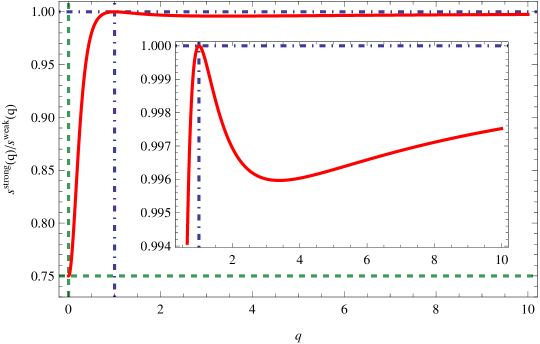
Figure 1: Ratio between Entanglement Rényi Entropies at strong coupling over weak coupling as a function of $q$. The green dashed line shows the limit of $q\rightarrow 0$, while the blue dashed-dotted line shows the result for Entanglement Entropy ($q\rightarrow 1$). The inset zooms near the region of $q\sim 1$.

As we see from figure 1, another interesting limit is $q\rightarrow 0$. The ratio between the ERE is exactly $3/4$ at this point. This factor is, of course, reminiscent of the $3/4$ that can be found in eq. (7) for the ratio between the strong and weak coupling results for the thermal free energy of ${\cal{N}}=4$ SYM. Examining the expression in eq. (5) more closely, one can see that in the limit of $q$ going to zero, the ERE must be proportional to the free energy of the theory in the plane. That is, when $q\rightarrow 0$, we have a divergent temperature $T_{0}/q\rightarrow\infty$. As the temperature goes to infinity, the curvature scale of the hyperbolic plane becomes negligible and then the free energy will simply grow as the fourth power of the temperature, i.e., as $q^{-4}$. Hence, in this limit, the term $F(T_{0}/q)$ dominates the expression in eq. (5) and we find $S_{q}\simeq-\frac{q}{T_{0}}F(T_{0}/q)=\frac{1}{4}S_{therm}(T_{0}/q)$ where both the free energy and the thermal entropy are evaluated in flat space here. Hence we recover the factor of $3/4$ observed previously in (flat space) thermal calculations for the ${\cal{N}}=4$ SYM theory peet . The discussion here provides a specific example of the general result that the $q\to 0$ limit of the ERE in any CFT is governed by the high temperature behaviour of the theory Swingle:2013hga .

Finally, it is also interesting to note that in the limit of $q\rightarrow\infty$, the ERE’s at strong and weak coupling coincide. We have no intuition for why the results agree in this low temperature limit and it appears that it is simply a coincidence which does not survive after finite coupling corrections are taken into account.

Knowing the results for the (universal contribution to the) ERE at both weak and strong coupling, we are ready to start the study of higher order corrections for the holographic calculations. From the study in this section, we should expect the ERE corrections to take certain specific values, at least, for $q\rightarrow 0$ and for $q\rightarrow 1$. For the former, we expect this correction to be equal to the correction to the free energy (as in eq. (7)), while for the latter we expect to find no correction.

3 ERE corrections

We start this section by discussing the first corrections to the standard supergravity action arising from the $\alpha^{\prime}$ expansion in type IIB superstring theory. It is known that the first corrections arise at the order $\alpha^{\prime 3}$, so that

$$I_{IIB}=I_{IIB}^{(0)}+\alpha^{\prime 3}\,I_{IIB}^{(1)}+\cdots,$$ (24)

where the $\cdots$ indicate terms involving higher powers of $\alpha^{\prime}$. Above, $I_{IIB}^{(0)}$ indicates the usual ten-dimensional effective action of type IIB supergravity john . Early studies of string scattering amplitudes curv4 and two-dimensional sigma-models curv4a indicated the appearance of quartic curvature interactions in $I_{IIB}^{(1)}$. It is also important to consider contributions of the Ramond-Ramond five-form to this action in order to properly determine the $\alpha^{\prime 3}$ corrections for phenomena in the AdS${}_{5}\times$ S⁵ compactification. These were carefully analyzed in Paulos:2008tn and it was shown that in general, $I_{IIB}^{(1)}$ depends on complicated combinations of the Weyl tensor and the Ramond-Ramond five-form in ten dimensions. However, examining the equations of motion showed that the higher order five-form terms all vanish for solutions of the form ${\cal A}_{5}\times$ S⁵, where ${\cal A}_{5}$ is a negatively curved Einstein manifold Myers:2008yi . In particular, the latter family of backgrounds would include the topological black holes in AdS, which are of interest here. Moreover, in Buchel:2008ae , the dimensional reduction to five dimensions of the pure curvature interaction in $I_{IIB}^{(1)}$ was analyzed, showing that it is consistent to work only with a reduced action constructed from the five-dimensional Weyl tensor. Hence for our holographic studies, it suffices to work with the following five-dimensional action:

$$I=I_{\text{bulk}}+\gamma\ I_{\text{Weyl}}\,,$$ (25)

where $I_{\text{bulk}}$ is the leading gravity action given in eq. (12). Further, $I_{\text{Weyl}}$ contains the interaction quartic in the Weyl curvature,

$$I_{\text{Weyl}}=\frac{L^{6}}{2\ell_{\textrm{\tiny P}}^{3}}\int d^{5}x\sqrt{-g}\ \ W\,,$$ (26)

with Gubser:1998nz ; Buchel:2004di

$$W=C^{hmnk}C_{pmnq}C_{h}^{\ rsp}C^{q}_{\ rsk}+\frac{1}{2}C^{hkmn}C_{pqmn}C_{h}^{\ rsp}C^{q}_{\ rsk}\ ,$$ (27)

where $C_{abcd}$ is the Weyl tensor in five dimensions

$$C_{abcd}=R_{abcd}-\frac{2}{3}\left(g_{a[c}R_{d]b}-g_{b[c}R_{d]a}\right)+\frac{1}{6}Rg_{a[c}g_{d]b}\,.$$ (28)

In eq. (25), the factor of $\alpha^{\prime 3}$ has been absorbed into the dimensionless coupling: $\gamma=\frac{1}{8}\zeta(3)\alpha^{\prime 3}/L^{6}$. Hence according to the standard AdS/CFT dictionary, this term in the gravity action will yield corrections of order $\lambda^{-3/2}$ in the description of the dual SYM theory. However, a more careful study of the origin of this higher curvature interaction instant allows one to argue that it also describes the corrections at order $\lambda^{1/2}/N^{2}$ Myers:2008yi — we return to this point in section 4.

Given the above action (25), we proceed as follows: In the next section, we calculate the $O(\gamma)$ corrections to the metric and Hawking temperature of the topological black hole that appeared in the holographic calculation of the ERE, as described in section 2.2. The ERE is related to the thermal free energy on the hyperbolic cylinder with eq. (5), which in turn is evaluated through the Euclidean on-shell action in the bulk gravitational theory. We evaluate the latter in two steps. First in section 3.2, we use the above perturbations of the metric and temperature to determine the $O(\gamma)$ correction to leading term in the action, $I_{\text{bulk}}$ (plus the corresponding boundary terms). Then in section 3.3, we determine the corrections to the ERE coming from $I_{\text{Weyl}}$. Since $I_{\text{Weyl}}$ already appears with a pre-factor $\gamma$, we can evaluate this on-shell action with the original black hole background. In the end, it turns out that this latter simpler calculation yields the entire correction to the ERE. Finally in section 3.4, we follow the discussion of Hung:2011nu to determine the $O(\gamma)$ corrections to the scaling dimension of the twist operators appearing in a standard calculation of the ERE.

3.1 The perturbed metric

In this subsection, we determine how the metric and the Hawking temperature are modified by including the $I_{\text{Weyl}}$ term in the action (25). As this interaction only represents the first term in an infinite expansion, we work perturbatively in $\gamma$ to find the corrections. We parametrize the perturbed metric as

$$ds^{2}= - \left(\frac{r^{2}}{L^{2}}\left(1-\frac{\omega^{4}}{r^{4}}\right)-1\right)\left(1+\gamma f_{2}(r)\right)\frac{L^{2}}{R^{2}}dt^{2}+$$ (29)

$$+\frac{dr^{2}}{\left(\frac{r^{2}}{L^{2}}\left(1-\frac{\omega^{4}}{r^{4}}\right)-1\right)\left(1+\gamma f_{3}(r)\right)}+r^{2}d\Sigma^{2}_{3},$$

where $f_{2}(r)$ and $f_{3}(r)$ are different functions that depend only on $r$. This parametrization was chosen so that the coordinate position of the horizon does not change, i.e., $r_{h}$ is the same function of $\omega$ as in eq. (15). To find the equations of motion for $f_{2}$ and $f_{3}$, we substitute the above metric into the action (25) and expand to second order in $\gamma$ — the first order variation vanishes identically, because the leading order background solves the original equations of motion. The resulting equations of motion for $f_{2}$ and $f_{3}$ are then

$$f_{3}^{\prime}(r) + \frac{2r\left(L^{2}-2r^{2}\right)}{L^{2}r^{2}-r^{4}+\omega^{4}}\ f_{3}(r)+$$ (30)

$$+ \frac{20\omega^{12}\left(160L^{2}r^{2}-144r^{4}+171\omega^{4}\right)}{r^{13}\left(L^{2}r^{2}-r^{4}+\omega^{4}\right)}+{\cal{O}}(\gamma)=0\,,$$

$$f_{2}^{\prime}(r) + \frac{2r\left(L^{2}-2r^{2}\right)}{L^{2}r^{2}-r^{4}+\omega^{4}}f_{3}(r)+\frac{20\omega^{12}\left(16L^{2}r^{2}+27\omega^{4}\right)}{r^{13}\left(L^{2}r^{2}-r^{4}+\omega^{4}\right)}+{\cal{O}}(\gamma)=0\,.$$

Solving for $f_{2}(r)$ and $f_{3}(r)$, we find

$$f_{2}(r) = \frac{5\omega^{12}\left(16L^{2}r^{2}-24r^{4}+9\omega^{4}\right)}{r^{12}\left(L^{2}r^{2}-r^{4}+\omega^{4}\right)}+\frac{C_{1}}{L^{2}r^{2}-r^{4}+\omega^{4}}+C_{2}\,,$$

$$f_{3}(r) = \frac{5\omega^{12}\left(64L^{2}r^{2}-72r^{4}+57\omega^{4}\right)}{r^{12}\left(L^{2}r^{2}-r^{4}+\omega^{4}\right)}+\frac{C_{1}}{L^{2}r^{2}-r^{4}+\omega^{4}}\,,$$ (31)

where $C_{1}$ and $C_{2}$ are integration constants. Examining the asymptotic metric, we see that $C_{2}$ simply produces a rescaling the time coordinate and since we want the solution to be asymptotically conformal to the boundary metric (14), we set $C_{2}$ to zero. To fix $C_{1}$, we notice that there is a potential divergence in $f_{2}(r_{h})$ and $f_{3}(r_{h})$ at the event horizon, i.e., at $r=r_{h}$ satisfying eq. (15). Then we choose $C_{1}$ to avoid these divergences,

$$C_{1}=\frac{5L^{4}}{x^{4}}\,\left(x^{2}-1\right)^{3}\left(15x^{2}-7\right)\,,$$ (32)

which is written in terms of the dimensionless parameter $x=r_{h}/L$. It is noteworthy that with this single choice, we avoid the potential singularities in both $f_{2}(r_{h})$ and $f_{3}(r_{h})$. Further, with this choice, we ensure that the coordinate position of the horizon remains at $r=r_{h}$.

We will also need the corrected Hawking temperature for this black hole geometry (29). It is calculated in the usual way and we obtain to first order in $\gamma$

$$T=T_{1}(x)\left(1+\frac{\gamma}{2}\left(f_{2}(r_{h})+f_{3}(r_{h})\right)+{\cal{O}}(\gamma^{2})\right),$$ (33)

where $T_{1}(x)$ is the zero’th order temperature given in eq. (17). Note that even though the coordinate position of the event horizon is not changed by the perturbation, the temperature receives a correction. As the holographic calculation of $S_{q}$ involves choosing the specific temperature $T_{0}/q$, we have to find the correction to the coordinate position of the event horizon that gives this fixed temperature at first order in $\gamma$. In terms of $x$, we have

$$\hat{x}_{q}=x_{q}-10\,\gamma\,\frac{\left(x_{q}^{2}-1\right)^{3}\left(1+3x_{q}^{2}\right)}{x_{q}^{6}\left(1+2x_{q}^{2}\right)}+{\cal{O}}\left(\gamma^{2}\right)\,,$$ (34)

where $x_{q}=\frac{1}{4q}\left(1+\sqrt{1+8q^{2}}\right)$ is the result determined previously for the unperturbed solution.

3.2 Corrections to ERE

Using eq. (5), we calculate the corrected ERE by evaluating the free energy at $T=T_{0}$ and $T_{0}/q$ (with $q$ any positive real number). In turn, the free energy is determined by evaluating the on-shell bulk action, which we do in two steps. First in this section, we use the above perturbations of the metric and temperature to determine the $O(\gamma)$ correction coming from the leading term in the action (25) and we leave the contribution from $I_{\text{Weyl}}$ to the next section. Of course, evaluating $I_{\text{bulk}}$ on-shell by itself yields a divergent result, which needs to be regularized. Holographic renormalization Henningson:1998gx ; Balasubramanian:1999re provides a framework for the latter, where boundary terms (that do not affect the equations of motion) are added to the usual action to produce a finite result. In Emparan:1999pm , it is shown that the full gravitational action (with Euclidean signature) can be written in terms of three contributions:

$$I_{\text{AdS}}=I_{\text{bulk}}(g_{ij})+I_{\text{surf}}(g_{ij})+I_{\text{ct}}(h_{ij})\,,$$ (35)

where $I_{\text{bulk}}$ is the Einstein-Hilbert action (25), $I_{\text{surf}}$ is the Gibbons-Hawking-York (GHY) term and $I_{\text{ct}}$ is the counterterm action, that is only a function of the boundary metric $h_{ij}$. If the bulk spacetime is five-dimensional with a four-dimensional boundary, the GHY and counterterm actions are given by

$$I_{\text{surf}} = -\frac{1}{\ell_{\textrm{\tiny P}}^{3}}\int_{\partial{\cal{M}}}d^{4}x\,\sqrt{h}\,K\ ,$$ (36)

$$I_{\text{ct}} = \frac{1}{\ell_{\textrm{\tiny P}}^{3}}\int_{\partial{\cal{M}}}d^{4}x\,\sqrt{h}\,\left[\frac{3}{L}+\frac{L}{4}{\cal{R}}\right]\,,$$

where $\partial{\cal{M}}$ corresponds to the boundary manifold with metric $h_{ij}$. Further, $K=h^{ij}\nabla_{i}n_{j}$ is the trace of the extrinsic curvature and ${\cal{R}}$ is the Ricci scalar for the induced boundary metric. Then the usual procedure is to evaluate the action with a cut-off surface at some large radius $R_{max}$. With this geometric cut-off, each of the contributions in eq. (35) is finite but the potential divergences cancel between the bulk and surface actions. Then taking the limit of $R_{max}\to\infty$ yields a finite result for the on-shell action and hence for the free energy.

Of course, in the following, we carry out all of these calculations to first order in $\gamma$. What we will find is that even though there are finite terms at first order coming from each of the different terms in the full action (35), once we combine these and write the final result as a function of temperature (or alternatively in terms of $q$), all of the $O(\gamma)$ contributions will be canceled. Hence, the only $O(\gamma)$ contribution to the ERE will be that coming from $I_{\text{Weyl}}$ in the next section. Here we might add that, as we will also see in the next section, $I_{\text{Weyl}}$ yields a finite result when evaluated on-shell and so no additional boundary terms are needed to regulate it.

First we show how the divergences cancel between the three terms in the action (35). To first order in $\gamma$, evaluating $I_{\text{bulk}}$ on-shell yields

$$I_{\text{bulk}}^{\text{on-shell}} = \beta\frac{V_{\Sigma_{3}}}{R}\left(\frac{L}{\ell_{\textrm{\tiny P}}}\right)^{3}\Bigg{(}-x^{4}+x_{\max}^{4}+$$

$$\left.+\gamma\left[\frac{15\left(1-9x^{2}\right)\left(x^{2}-1\right)^{3}}{2x^{4}}+{{O}}\left(\frac{1}{x_{\max}}\right)\right]+{{O}}\left(\gamma^{2}\right)\right)\,,$$

where $x_{max}\equiv R_{max}/L$. In the end, we take $x_{max}$ to infinity and so we do not need to keep track of the ${{O}}\left(x_{\max}^{-1}\right)$ terms. Note that eq. (3.2) still contains a finite term at order $\gamma$, which can be seen as coming from a boundary term at the horizon. For the GHY term, we obtain

$$I_{\text{surf}}^{\text{on-shell}} = \beta\frac{V_{\Sigma_{3}}}{R}\left(\frac{L}{\ell_{\textrm{\tiny P}}}\right)^{3}\Bigg{(}2x^{2}\left(x^{2}-1\right)+3x_{\max}^{2}-4x_{\max}^{4}+$$ (38)

$$\left.+\gamma\left[\frac{10\left(15x^{2}-7\right)\left(x^{2}-1\right)^{3}}{x^{4}}+{{O}}\left(\frac{1}{x_{\max}}\right)\right]+{{O}}\left(\gamma^{2}\right)\right)\,.$$

Again, this boundary contribution contains divergent terms at zero’th order, i.e., the $x_{max}^{2}$ and $x_{max}^{4}$ terms, but only finite terms at first order in $\gamma$. Finally, the counterterm action yields

$$I_{\text{ct}}^{\text{on-shell}} = \beta\frac{V_{\Sigma_{3}}}{R}\left(\frac{L}{\ell_{\textrm{\tiny P}}}\right)^{3}\Bigg{(}\frac{3}{8}\left(1+4x^{2}-4x^{4}\right)+3x_{\max}^{4}-3x_{\max}^{2}+{{O}}\left(\frac{1}{x_{\max}}\right)+$$ (39)

$$\left.+\gamma\left[\frac{15\left(15x^{2}-7\right)\left(x^{2}-1\right)^{3}}{2x^{4}}+{{O}}\left(\frac{1}{x_{\max}}\right)\right]+{{O}}\left(\gamma^{2}\right)\right)\,.$$

Note that this counterterm action not only cancels the divergences arising from the bulk and surface actions but it also introduces an $x$-dependent term to the action at zero’th order, i.e. $O(\gamma^{0})$. Again, there are no divergences but a finite contribution appears at first order. The fact that no divergences appear at first order in any of these three actions is closely related to the fact that both $f_{2}$ and $f_{3}$ decay rapidly with $r$ and so at the boundary, their contributions are highly suppressed.

Combining all three contributions above and dividing by $\beta$, we find the free energy $F=I/\beta$ is given by

$$F(x)=\frac{V_{\Sigma_{3}}}{R}\left(\frac{L}{\ell_{\textrm{\tiny P}}}\right)^{3}\left(\frac{3}{8}-\frac{x^{2}}{2}(1+x^{2})-\gamma\,\frac{10\left(x^{2}-1\right)^{3}\left(3x^{2}+1\right)}{x^{4}}\right)\,.$$ (40)

Now this result can be used in eq. (5) to determine the contributions of $I_{\text{bulk}}$ to the ERE. Hence we recall that for $T=T_{0}$, $x=1$ while for $T=T_{0}/q$, $x$ is defined to be $\hat{x}_{q}$ as given in eq. (34) to first order in $\gamma$. Combining these results, the ERE becomes

$$S_{q}=\frac{\pi q}{q-1}V_{\Sigma_{3}}\left(\frac{L}{\ell_{\textrm{\tiny P}}}\right)^{3} \Bigg{[} 2-\hat{x}_{q}^{2}(1+\hat{x}_{q}^{2})+$$

$$- \gamma\frac{20\left(x_{q}^{2}-1\right)^{3}\left(3x_{q}^{2}+1\right)}{x_{q}^{4}}+{{O}}\left(\gamma^{2}\right)\Bigg{]}\,,$$

where we still do not incorporate the contribution from $I_{\text{Weyl}}$. Of course, the zero’th order term has precisely the expected form as given in eq. (21) from the previous calculations. However, note that this expression is written in terms of $\hat{x}_{q}$ (rather than $x_{q}$), which contains an $O(\gamma)$ term as shown in eq. (34). Therefore a first order correction is hidden in this ‘zero’th order’ term, i.e.,

$$\left.-\hat{x}_{q}^{2}\left(1+\hat{x}_{q}^{2}\right)\right|_{\gamma}=\gamma\frac{20\left(x_{q}^{2}-1\right)^{3}\left(3x_{q}^{2}+1\right)}{x_{q}^{4}}.$$ (42)

Comparing the above expression with the explicit $O(\gamma)$ term in eq. (3.2), we see that the two corrections precisely cancel. Hence the final contribution here to the ERE is given by

$$S_{q}=\frac{\pi q}{q-1}V_{\Sigma_{3}}\left(\frac{L}{\ell_{\textrm{\tiny P}}}\right)^{3} \Bigg{[} 2-x_{q}^{2}(1+x_{q}^{2})+{{O}}\left(\gamma^{2}\right)\Bigg{]}.$$ (43)

The corresponding universal contribution to the ERE is given by precisely the same expression as in eqs. (22) and (23). However, remember that here we have not yet taken into account the contribution from the Weyl term (26), which will be considered in the next section.

3.3 More corrections to ERE

In the previous section, we reproduced the contribution to ERE in eq. (21), which was found with simply the Einstein action (12). However, the calculation there included the $O(\gamma)$ corrections to the metric and Hawking temperature found in section 3.1 and there was a cancelation at this order which left $S_{q}$ unchanged. This result is incomplete though since we still have to account for the contribution coming from $I_{\text{Weyl}}$. We calculate this correction in the following.

Since this term already appears with a pre-factor $\gamma$ in eq. (25), it suffices to evaluate it on-shell the uncorrected metric (13). That is, any $O(\gamma)$ perturbation in the metric will introduce a $\gamma^{2}$ term when included in $I_{\text{Weyl}}$. For the same reason when evaluating the ERE with eq. (5), we can also use $x_{q}$ as given in eq. (20), without the $O(\gamma)$ corrections appearing in eq. (34).

Now, it is useful to note that $W$ can be written in the form Buchel:2004di

$$W=B_{ijkl}\left(2B^{iklj}-B^{lijk}\right),\ \ \ \ \ \ B_{ijkl}=C^{m}{}_{ijn}\,C^{n}{}_{lkm}\,.$$ (44)

Then, evaluating eq. (44) with the zero’th order metric (13) yields

$$W=\frac{180}{L^{8}}\frac{\omega^{16}}{r^{16}}\,.$$ (45)

This is quite similar to the result obtained for the planar AdS black hole Gubser:1998nz , with the difference that now $\omega$ is not $r_{h}$ but instead, it is given by eq. (15). Note that $W$ scales as $r^{-16}$, so even with the $r^{3}$ coming from the determinant of the metric, $I_{\text{Weyl}}$ will yield a finite result without any need of regularization. After integrating then, we find

$$I_{\text{Weyl}}=-\beta\frac{15}{2}\frac{V_{\Sigma_{3}}}{R}\left(\frac{L}{\ell_{\textrm{\tiny P}}}\right)^{3}\frac{(1-x^{2})^{4}}{x^{4}}\,.$$ (46)

Now let us denote $\delta F=I_{\text{Weyl}}/\beta$, which takes the form

$$\delta F=-\frac{15}{2}\frac{V_{\Sigma_{3}}}{R}\left(\frac{L}{\ell_{\textrm{\tiny P}}}\right)^{3}\frac{(1-x^{2})^{4}}{x^{4}}$$ (47)

To determine the corresponding contribution in eq. (5), we just evaluate this expression at $x=1$ and at $x=x_{q}$. It is interesting to note that at $x=1$, i.e., $r_{h}=L$, $I_{\text{Weyl}}$ vanishes. This vanishing can be anticipated because when $T$ is exactly $T_{0}$, the topological black hole solution is in fact just the pure AdS spacetime Casini:2011kv , for which the Weyl curvature vanishes. Evaluating the correction to ERE results in the following universal contribution

$$\delta S^{\log}_{q}(R)=-8\gamma\,N^{2}\,s^{(1)}(q)\,\log\left(\frac{R}{\delta}\right)\,,$$ (48)

with

$$s^{(1)}(q) = -\frac{15}{16}\frac{q}{q-1}\frac{(1-x_{q}^{2})^{4}}{x_{q}^{4}}$$ (49)

$$= 15\frac{(1+q)(1-q^{2})^{3}}{q^{3}\,(3+\sqrt{1+8q^{2}})^{4}}\,.$$

The final expression above was again chosen to make obvious that there is no singularity at $q=1$. Given the cancelation found in the previous section, the above result is the entire $O(\gamma)$ correction to the ERE.

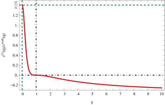
Figure 2: Correction to the ERE due to $\alpha^{\prime 3}$ effects. Again, the green dashed line shows the limit of $q\rightarrow 0$, while the blue dashed-dotted line shows the result for entanglement entropy ($q=1$).

In figure 2, we show $s^{(1)}(q)/s^{\text{weak}}(q)$ as a function of $q$. We might note that the result for the corrections to ERE can be anticipated in the two limits. First as explained in section 2.2, the ERE reduces to the entanglement entropy at $q=1$ and since the universal contribution to the latter is determined by the central charge $a$, it must be independent of the ‘t Hooft coupling. Hence the correction term (48) vanishes at $q=1$, as it is evident from the factor of $(1-q^{2})^{3}$ appearing in eq. (49). The second case, where the result can be anticipated is $q\to 0$, for which we find $s^{(1)}(0)/s^{\text{weak}}(0)=45/32$. As also discussed in section 2.2, the ERE is proportional to the flat space free energy in this limit. Hence this fraction is precisely the pre-factor appearing in the $O(\lambda^{-3/2})$ correction to the free energy appearing in eq. (7).

Another interesting limit to consider is $q\rightarrow\infty$, for which $s^{(1)}(\infty)/s^{\text{weak}}(\infty)=-3/8$. As was noted previously, even though the leading terms at weak and at strong coupling coincide in this limit, there is no obvious reason to believe that there should be no coupling dependence. The fact that the correction (48) is not vanishing in this limit seems to indicate that the match found at leading order was merely a coincidence.

3.4 Scaling dimension of twist operators

Our holographic calculations of the ERE for a spherical entangling surface take advantage of mapping the problem to a thermodynamic one, as described in Casini:2011kv — see also cthem . This approach contrasts with ‘standard’ field theoretic computations which make use of the replica trick, e.g., cardy0 . In this approach, one considers a path integral over $q$ replicas or copies of the original QFT and inserts twist operators which open branch cuts between between these copies at the entangling surface. In two dimensions, the twist operators are local conformal primary fields cardy0 but in higher dimensions, they become ($d-2$)-dimensional surface operators. In practice the construction and properties of these operators are not well understood for $d>2$. However, following Hung:2011nu , we can use the thermal calculation for the ERE to determine their scaling dimension $h_{q}$, in particular for holographic CFT’s.

The scaling dimension $h_{q}$ for twist operators $\sigma_{q}$ in a four-dimensional CFT is defined as follows: in flat Euclidean space, consider a planar twist operator positioned at $x^{1}=0=x^{2}$ while it extends throughout the remaining $x^{3}$ and $x^{4}$ directions. Now make an insertion of the stress tensor operator at $x^{\mu}=\{y^{1},y^{2},y^{3},y^{4}\}$ and define the orthogonal distance between the two operators as $r^{2}=(y^{1})^{2}+(y^{2})^{2}$. Then the leading singularity in the corresponding correlator takes the following form

$$\langle T_{ab}\,\sigma_{q}\rangle = -\frac{h_{q}}{2\pi}\,\frac{\delta_{ab}}{r^{4}}\,,\qquad\langle T_{ai}\,\sigma_{q}\rangle=0\,,$$

$$\langle T_{ij}\,\sigma_{q}\rangle = \frac{h_{q}}{2\pi}\,\frac{3\,\delta_{ij}-4\,n_{i}\,n_{j}}{r^{4}}\,.$$ (50)

where $i,j=\{1,2\}$, $a,b=\{3,4\}$ and $n^{i}=y^{i}/r$ is the unit vector directed orthogonally from the twist operator to the $T_{\mu\nu}$ insertion. Note that the form of this result is completely fixed by translation and rotation symmetries, as well as $\langle T^{\mu}{}_{\mu}\,\sigma_{q}\rangle=0=\nabla^{\mu}\langle T_{\mu\nu}\,\sigma_{q}\rangle$. Further note that the correlators in eq. (50) are implicitly normalized by dividing out by $\langle\sigma_{q}\rangle$ but we left this normalization implicit to avoid the clutter. Finally, let us add that we assume that $T_{\mu\nu}$ corresponds to the total stress tensor for the entire $q$-fold replicated CFT, i.e., $T_{\mu\nu}$ is inserted on all $q$ sheets of the universal cover.

Now as described in Hung:2011nu , the conformal mapping between the thermal state at temperature $T_{0}/q$ on the hyperbolic cylinder and the $q$-fold cover of $R^{4}$ allows us to describe the leading singularity in eq. (50) and in particular, the scaling weight in terms of the thermal properties of the CFT. The final result for $d=4$ is Hung:2011nu

$$h_{q}=\frac{2\pi}{3}\ q\ R^{4}\left({\cal{E}}(T_{0})-{\cal{E}}(T_{0}/q)\right)\,,$$ (51)

where ${\cal{E}}=E/(R^{3}V_{\Sigma_{3}})$ is the energy density of the thermal state on $R\times H^{3}$. Our holographic calculations in the preceding sections have determined the free energy and the temperature for SYM on the hyperbolic cylinder and so it is straightforward to evaluate the scaling dimension of the twist operators, including the leading corrections, using the standard thermodynamic relation, $E=F-T\ \partial F/\partial T$. The final result takes the form

$$h_{q} = \pi\left(\frac{L}{\ell_{\textrm{\tiny P}}}\right)^{3}q\ x_{q}^{2}\left(1-x_{q}^{2}\right)$$ (53)

$$\qquad\times\left(1+5\gamma\,\frac{\left(1-x_{q}^{2}\right)^{2}\left(-3+5x_{q}^{2}+6x_{q}^{4}\right)}{x_{q}^{6}\left(1+2x_{q}^{2}\right)}+\cdots\right)$$

$$= -\frac{\pi}{q^{3}}\left(\frac{L}{\ell_{\textrm{\tiny P}}}\right)^{3}\Bigg{(}\frac{1}{32}\,\frac{(1+\sqrt{1+8q^{2}})^{3}}{3+\sqrt{1+8q^{2}}}(1-q^{2})+$$

$$\qquad\quad+\ 10\,\gamma\,\frac{8q^{2}-3+9\sqrt{1+8q^{2}}}{\sqrt{1+8q^{2}}\,(3+\sqrt{1+8q^{2}})^{3}}(1-q^{2})^{3}+\cdots\Bigg{)}\,.$$

The expression in the final line was chosen to make manifest the zero at $q=1$. The leading order term above applies for any four-dimensional CFT dual to Einstein gravity in the bulk and is the same as the result reported in Hung:2011nu .

Examining the leading order result for $h_{q}$ for a broad class of holographic theories in Hung:2011nu , it was observed that with $d=4$

$$\partial_{q}h_{q}|_{q=1}=\frac{2}{3\pi}\,c\,.$$ (54)

Recall that for ${\cal N}=4$ SYM with a $SU(N)$ gauge group, the two central charges are given by $c=a=N^{2}/4$, in the large $N$ limit. From eq. (53), we observe that the $O(\gamma)$ correction to $\partial_{q}h_{q}|_{q=1}$ vanishes, providing evidence that the expression in eq. (54) is independent of the coupling. In fact, in twistop , it was shown that eq. (54) is a general formula which holds for any CFT. That is, this result does not rely on strong coupling, large $N$ or even holography. Therefore since the central charges are protected by supersymmetry in SYM, eq. (54) can not receive any $\lambda$ dependent corrections and so the $O(\gamma)$ correction from eq. (53) was required to vanish in evaluating $\partial_{q}h_{q}|_{q=1}$. As is evident from eq. (53), i.e., from the factor of $(1-q^{2})^{3}$, the $O(\gamma)$ correction also vanishes for $\partial^{2}_{q}h_{q}|_{q=1}$ but is nonvanishing for higher derivatives of the scaling weight. This observation can again be related to further results found in twistop . There, the conformal mapping between the ERE for a spherical entangling surface and the thermal state on the hyperbolic cylinder was used to show that $\partial^{n}_{q}h_{q}|_{q=1}$ can be related to $n$- and $(n+1)$-point correlation functions of the stress tensor. Hence $\partial^{2}_{q}h_{q}|_{q=1}$ is determined by the two- and three-point function of the stress tensor. In the SYM theory, the parameters controlling these correlators are still protected by supersymmetry and so the $O(\gamma)$ contribution from eq. (53) is required to vanish. In contrast, the higher derivatives of $h_{q}$ receive $O(\gamma)$ corrections, in accord with the expectation that the corresponding higher point functions of the stress tensor will depend on the ‘t Hooft coupling.

4 Discussion and conclusions

In this paper, we have used holography to examine the entanglement Rényi entropies for a spherical entangling surface in the ${\cal{N}}=4$ SYM theory at strong coupling and large $N$. In particular, we have determined the leading finite $\lambda$ (and finite $N$) corrections arising from higher curvature corrections in the effective type IIB gravity action. Our results in the main text were expressed in terms of a dimensionless expansion parameter $\gamma=\frac{1}{8}\zeta(3)\,\alpha^{\prime 3}/L^{6}$, which the standard AdS/CFT dictionary translates to $\gamma=\frac{1}{8}\zeta(3)\,\lambda^{-3/2}$ in the dual SYM theory. However, a careful examination of the origin of the higher curvature interaction (26) reveals that the pre-factor actually involves a modular form instant ; Paulos:2008tn . The latter captures the behaviour for all values of the string coupling but remarkably contains only string tree-level and one-loop contributions at weak coupling, as well as an infinite series of instanton corrections. The tree-level term corresponds to the $O(\lambda^{-3/2})$ correction but the one-loop term yields a new correction at order $O(\lambda^{1/2}/N^{2})$ Myers:2008yi . Hence our calculations also capture the leading finite $N$ corrections which appear at this order. Note that this additional correction is enhanced by a factor of $\lambda^{1/2}$ over what the naive large $N$ counting suggests would appear as the first corrections. Combining the results in the main text then, we find that the universal contribution to the ERE for a spherical entangling surface in the ${\cal{N}}=4$ SYM theory at strong coupling and large $N$, behaves as

$$S^{\log}_{q}(R)=-N^{2}\log\left(\frac{R}{\delta}\right)\,\left[s^{(0)}(q)+\left(\frac{\zeta(3)}{\lambda^{3/2}}+\frac{\lambda^{1/2}}{48N^{2}}\right)s^{(1)}(q)+\cdots\right]$$ (55)

where

$$s^{(0)}(q) = \frac{1+q}{64q^{3}}\,\frac{(5\sqrt{1+8q^{2}}-3)(1+\sqrt{1+8q^{2}})^{2}}{3+\sqrt{1+8q^{2}}}\,,$$ (56)

$$s^{(1)}(q) = 15\frac{(1+q)(1-q^{2})^{3}}{q^{3}\,(3+\sqrt{1+8q^{2}})^{4}}\,.$$

One interesting observation in section 3 was that when the metric with first order corrections was used to evaluate the contribution to the ERE coming from the on-shell $I_{\text{bulk}}$, there was a cancelation at $O(\gamma)$ and our final result took the same form (21) as without considering the corrections. A similar result was found in Gubser:1998nz when calculating the leading corrections to the free energy for the planar AdS black hole. In fact, general arguments indicate this behaviour will always occur in a perturbative calculation of the type which we considered. Imagine evaluating the on-shell action for a perturbed metric $(g_{0}+\gamma\,g_{1})_{ij}$, as follows

$$I(g_{0}+\gamma g_{1}) = I_{0}(g_{0}+\gamma g_{1})+\gamma I_{1}(g_{0}+\gamma g_{1})+\cdots$$ (57)

$$= I_{0}(g_{0})+\left.\frac{\delta I_{0}}{\delta g_{ij}}\right|_{g_{0}}\gamma\,(g_{1})_{ij}+\gamma I_{1}(g_{0})+\cdots$$

$$= I_{0}(g_{0})+\gamma I_{1}(g_{0})+\cdots\,,$$

where $\cdots$ indicate higher order terms in the expansion. Between the second and third lines we used that the variation of $I_{0}$ vanishes when evaluated on a solution to the zero’th order equations of motion. However, there is some subtetly in this argument, because the variation is actually only zero up to total derivative terms. In fact, one can show that the extra terms appearing at the leading order, e.g., in eq. (3.2) for the bulk action, are total derivatives. So why then do we find the cancelation at $O(\gamma)$ in the final result. First, the profile of the perturbation decays rapidly and so the boundary contribution produced by the total derivative vanishes at asymptotic infinity. The other ‘boundary’ to consider at the horizon but in fact, the temperature is chosen to ensure that the Euclidean geometry is smooth there, i.e., there is no boundary at $r=r_{h}$. The appearance of apparent contributions at this internal boundary arises because our perturbative construction does not enforce this smoothness at every step. However, as shown in section 3.2, when all of the intermediate results are combined, the extra “total derivative” terms cancel in the final result and we are only left with $I_{1}(g_{0})=I_{\text{Weyl}}(g_{0})$ giving the full correction, as in eq. (57). It seems that it is important that this simple general argument of expanding the action should only be applied to the case of the renormalized (i.e., the finite) action. We note again that the same thing happens in Gubser:1998nz . The bulk action appears to receive corrections from the perturbed metric but after properly regularizing and combining with the surface terms, the final result is independent of the metric perturbation.

A consistency check of our results is given in appendix A, where we calculate ERE using a horizon entropy approach. The latter proceeds by calculating the corrected horizon entropy, using Wald’s formula Wald , and Hawking temperature and then using eq. (6) to determine the ERE. We show that this approach yields precisely the same results as found in the main text. The advantage of this method is that one does not need to consider surface terms and the holographic renormalization of the action in order to get finite results. However, one still needs to calculate metric perturbations as in section 3.1 to get the temperature to first order in $\gamma$ and then integrate eq. (6) to get ERE.

The latter also provides some insight on the behaviour of the corrections to the ERE in eq. (55). In particular, we note that $s^{(1)}(q)$ vanishes the limit $q\to 1$ and actually, it has a cubic zero at this point, as shown in eq. (56). Now in the horizon entropy approach, the correction to the ERE is determined by the correction to the horizon entropy arising from $I_{\text{Weyl}}$ and as we showed in appendix A, the latter is cubic in the Weyl tensor. Further, the result at $q=1$ corresponds precisely to the horizon entropy of the topological black hole with $T=T_{0}$, but the latter background is, in fact, precisely the AdS vacuum solution for which $C_{abcd}=0$! Hence this vanishing of the Weyl curvature and the cubic dependence of the Wald entropy on $C_{abcd}$ can be seen as the gravitational origin of the behaviour of $s^{(1)}(q)$ around $q=1$, which we noted above.

In part, our study was motivated by the fact that ERE were calculated for SYM previously at both strong coupling Hung:2011nu and weak coupling Fursaev:2012mp , but the results did not match in general. We reviewed these previous calculations and compared the results in section 2. Of course, for such a comparison, we must focus on the universal log term in the ERE and implicitly, we will be referring to this contribution throughout the following.

With $q=1$, the ERE reduces to the entanglement entropy and the leading results at strong and weak coupling were shown to agree in section 2. As noted there, this agreement is expected since in this case, the universal coefficient is determined by the central charge $a$, which is protected by supersymmetry in SYM. Of course then, this agreement at $q=1$ persists beyond the leading order for the final result (55), which also includes the finite $\lambda$ and finite $N$ corrections. These terms have the potential to introduce dependence of the EE on the ’t Hooft coupling but as is evident from eq. (56), $s^{(1)}(q=1)=0$ and there are no higher order corrections to the EE.

Another case where the leading results in section 2 were found to agree in the strong and weak coupling limits was with $q\rightarrow\infty$. However, there was no obvious reason to believe that the universal coefficient in the ERE should be independent of the coupling in this limit. Our calculation of the higher order corrections confirmed that this match at leading order was only a coincidence. In particular, we see that $s^{(1)}(q\to\infty)=-15/64$ from eq. (56) and so there is an explicit $\lambda$ dependence in this limit for the ERE given in eq. (55).

The final case where an interesting analytic comparison could be made between strong and weak coupling was in the limit $q\to 0$. In this limit, the ERE is probing the high temperature behaviour of the SYM theory. As seen with $T_{0}/q\to\infty$ in eqs. (5) and (6), the dominant contribution becomes $S_{q}\simeq-\frac{q}{T_{0}}F(T_{0}/q)=\frac{1}{4}S_{therm}(T_{0}/q)$ where both the free energy and the thermal entropy can be evaluated in flat space since the curvature scale of the hyperbolic plane becomes negligible in this limit. Again we note that this is a specific example of the general result recently discussed in Swingle:2013hga . Comparing the strong and weak coupling results in section 2, we find $s^{\text{strong}}(0)/s^{\text{weak}}(0)=3/4$, which is precisely the famous factor of $3/4$ found in comparing the thermal entropy at strong and weak coupling for ${\cal{N}}=4$ SYM peet . This matching also extends to the higher order corrections found in section 3. There we found $s^{(1)}(0)/s^{\text{weak}}(0)=45/32$, which is precisely the prefactor found for the $O(\lambda^{-3/2})$ correction to the thermal entropy in eq.(7). In fact, at weak coupling, we should also see the same leading correction as in eq. (8) appearing as the first correction for $s^{\text{weak}}(q\to 0)$ at $O(\lambda)$.

Examining the comparison of the leading results for strong and weak coupling shown in figure 1, we see that in general $s^{\text{strong}}(q)$ tends to be smaller than $s^{\text{weak}}(q)$. As discussed above, the exceptions are $q=1$ and $q\to\infty$ where the two universal coefficients coincide, but it is interesting to note that for no value of $q$ do we ever find $s^{\text{strong}}(q)>s^{\text{weak}}(q)$. Further, while both of these coefficients are positive throughout the full range of $q$, in figure fig 2 or eq. (56), we see that $s^{(1)}(q)=s^{\text{Weyl}}(q)$, the coefficient of the higher order corrections at strong coupling, changes sign at $q=1$. In particular, for $q<1$, the correction to ERE is positive and so one can imagine that as a function of the ‘t Hooft coupling, it is rising from the strong coupling result towards the weak coupling answer, as depicted in figure 3a. This is similar to the situation for the thermal entropy, described around eqs. (7–8). As discussed above, at precisely $q=1$, the universal coefficient is independent of the coupling and so the higher order corrections to the ERE vanish. Of course, we also have $s^{(1)}(q)<0$ for $q>1$. This means that in this range of $q$, the first corrections at the strong coupling are actually taking the ERE farther away from the weak coupling limit, as shown in figure 3c. While this does not produce any inconsistency, the situation is perhaps slightly unusual. It would be interesting to determine the corrections given by perturbation theory for small coupling, or even the next term coming from the holographic calculations at strong coupling, to have a more concrete idea of how ERE behaves as a function of $\lambda$. In particular, in figure 3, we have assumed that ERE is a smooth function interpolating between the strong and weak coupling limits, but it would interesting if instead there was a phase transition at some intermediate value of the coupling.

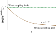
(a) $q<1$

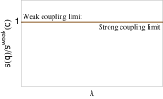
(b) $q=1$

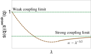
(c) $q>1$

Figure 3: Schematic behaviour of ERE as a function of ’t Hooft coupling for different values of $q$. In each plot $q$ is fixed. For $q<1$, the first order correction at strong coupling is positive; for $q=1$, there is no correction as the EE is independent of $\lambda$; for $q>1$, the correction is negative.

Lastly, in section 3.4, we also calculated the the scaling dimension of twist operators involved in calculating the ERE. Our calculations followed the approach given in Hung:2011nu , using the thermal energy density on the hyperbolic cylinder. Our holographic calculations reproduced the leading strong coupling result found in Hung:2011nu , but we also found the leading finite $\lambda$ and finite $N$ corrections for the SYM theory. Expressed in terms of the boundary theory parameters, the scaling weight (53) becomes

$$h_{q} = -\frac{N^{2}}{4\pi q^{3}}\Bigg{(}\frac{1}{32}\,\frac{(1+\sqrt{1+8q^{2}})^{3}}{3+\sqrt{1+8q^{2}}}(1-q^{2})+$$

$$\qquad\quad+\ \frac{10}{8}\,\left(\frac{\zeta(3)}{\lambda^{3/2}}+\frac{\lambda^{1/2}}{48N^{2}}\right)\,\frac{8q^{2}-3+9\sqrt{1+8q^{2}}}{\sqrt{1+8q^{2}}\,(3+\sqrt{1+8q^{2}})^{3}}(1-q^{2})^{3}+\cdots\Bigg{)}\,.$$

Further following the discussion of Hung:2011nu ; twistop , it was observed above that this result satisfies certain identities which are protected by supersymmetry. For example, as given in eq. (54), we have $\partial_{q}h_{q}|_{q=1}=\frac{N^{2}}{6\pi}$ and a similar identity will hold for $\partial^{2}_{q}h_{q}|_{q=1}$. The coupling independence of these expressions results from the factor of $(1-q^{2})^{3}$ in higher order contributions in eq. (4). The higher derivatives of $h_{q}$ receive finite $\lambda$ (and finite $N$) corrections because the coupling independence expectation does not extend the corresponding higher point functions of the stress tensor. At present, there are no comparable results at weak coupling with which we can compare this scaling weight (4) at strong coupling. We observe that the approach for calculating $h_{q}$ in Hung:2011nu does not rely on holography and so could equally well be applied to SYM at weak coupling, e.g., using heat kernel techniques. This would, of course, be an interesting project for future work.

Appendix A A horizon entropy approach to ERE

The aim of this Appendix is to provide an alternative way to calculate ERE. As shown in eq. (6), one can obtain the ERE by knowing the behaviour of both the thermal entropy and the temperature. Integrating by parts in eq. (6) and writing the result in terms of variable $x$, we find Hung:2011nu

$$S_{q}=\frac{q}{q-1}\frac{1}{T_{0}}\left(\left.S(x)T(x)\right|^{1}_{x_{q}}-\int_{x_{q}}^{1}\frac{dS}{dx}T(x)dx\right).$$ (59)

Of course, the thermal entropy corresponds to the horizon entropy in the dual gravity theory. For theories with higher curvature interactions, one must evaluate the Wald entropy Wald

$$S=-2\pi\int_{\text{horizon}}d^{3}x\ \sqrt{h}\ \frac{\partial{\cal{L}}}{\partial R_{abcd}}\ \hat{\varepsilon}_{ab}\,\hat{\varepsilon}_{cd}\,,$$ (60)

where ${\cal{L}}$ is the Lagrangian for the particular gravitational theory under consideration and $\hat{\varepsilon}_{ab}$ is the volume form in the two-dimensional space transverse to the bifurcation surface of horizon. The latter is normalized so that $\hat{\varepsilon}_{ab}\hat{\varepsilon}^{ab}=-2$. Of course, for Einstein gravity with ${\cal{L}}=R/(2\ell_{\textrm{\tiny P}}^{3})$, this expression (60) reduces to the Bekenstein-Hawking area law, i.e., $S=2\pi{\cal A}/\ell_{\textrm{\tiny P}}^{3}$. However, in the present case, we also need to analyze the contribution coming from $I_{\text{Weyl}}$ in eq. (26). To incorporate this correction we first note that the geometry at the horizon is homogeneous, so we may simplify eq. (60) as

$$S=-2\pi\ r_{h}^{3}\ V_{\Sigma_{3}}\ \left.\frac{\partial{\cal{L}}}{\partial R_{abcd}}\ \hat{\varepsilon}_{ab}\,\hat{\varepsilon}_{cd}\right|_{r=r_{h}}.$$ (61)

Now given the five-dimensional action (25), we have

$${\cal{L}}=\frac{1}{2\ell_{\textrm{\tiny P}}^{3}}(R+\gamma W),$$ (62)

where we recall that $W$ is given by

$$W = C^{hmnk}C_{pmnq}C_{h}^{\ rsp}C^{q}_{\ rsk}+\frac{1}{2}C^{hkmn}C_{pqmn}C_{h}^{\ rsp}C^{q}_{\ rsk}\ ,$$ (63)

with

$$C_{abcd} = R_{abcd}-\frac{1}{3}\left(g_{ac}R_{db}-g_{ad}R_{cb}-g_{bc}R_{da}+g_{bd}R_{ca}\right)+\frac{1}{12}R(g_{ac}g_{db}-g_{ad}g_{cb})\,.$$ (64)

To compute the variation with respect to $R_{abcd}$ in eq. (61), it is easiest to first vary with respect to the Weyl tensor and then with respect to the Riemann tensor, i.e.,

$$\frac{\partial{\cal{L}}_{\text{Weyl}}}{\partial R_{abcd}}=\frac{\partial{\cal{L}}_{\text{Weyl}}}{\partial C_{efgh}}\cdot\frac{\partial C_{efgh}}{\partial R_{abcd}}\,.$$ (65)

This is a rather tedious but straightforward calculation. Basically, each of the $C$’s in $W$ will contribute with one term to the first variation above, while each $R$, $R_{ab}$, $R_{abcd}$ will contribute with one term to the second one. So in total we find 48 different terms. For example, the first term corresponds to taking the derivative with respect to the first Weyl tensor in eq. (63) and with respect to the first $R_{abcd}$ in eq. (64) to produce

$$\left(\left.\frac{\partial{\cal{L}}_{\text{Weyl}}}{\partial R_{abcd}}\hat{\varepsilon}_{ab}\hat{\varepsilon}_{cd}\right|_{r=r_{h}}\right)_{I}=\left.C_{pmnq}C_{h}^{\ rsp}C^{q}_{\ rsk}\hat{\varepsilon}^{hm}\hat{\varepsilon}^{nk}\right|_{r=r_{h}}=-84\ \frac{\omega^{12}}{r_{h}^{\ 12}}.$$ (66)

All the non vanishing terms yield an expression proportional to ${\omega^{12}}/{r_{h}^{\ 12}}$ when evaluated on the topological black hole solution and so one only has to sum all the different contributions. In all, writing the result in terms of $x$ instead of $r_{h}$ yields

$$S(x)=2\pi V_{\Sigma_{3}}\left(\frac{L^{3}}{\ell_{\textrm{\tiny P}}^{3}}\right)x^{3}\left(1+60\gamma\frac{(x^{2}-1)^{3}}{x^{6}}\right).$$ (67)

Notice that the zero’th order term is exactly the same as that in eq. (18). To compare our previous results with eq. (67), it is simply to translate the free energy found in the main text into the corresponding thermal entropy using

$$S=-\frac{\partial F}{\partial T}=-{\frac{\partial F}{\partial x}}\,\bigg{/}\,{\frac{\partial T}{\partial x}}\,.$$ (68)

Having the expressions of both the free energy and the temperature to first order in eqs. (46) and (33), we can compute the thermal entropy to first order in $\gamma$ and we find that we reproduce precisely eq. (67). Of course, if one gets the same entropy in both cases, then the calculation for ERE must also agree.

References

-
(1)
M. Levin and X.-G. Wen,
“Detecting Topological Order in a Ground State Wave Function,”
Phys. Rev. Lett. 96, 110405 (2006)
[arXiv:cond-mat/0510613];
A. Kitaev and J. Preskill, “Topological entanglement entropy,” Phys. Rev. Lett. 96, 110404 (2006) [arXiv:hep-th/0510092];
A. Hamma, R. Ionicioiu and P. Zanardi, “Ground state entanglement and geometric entropy in the Kitaev’s model,” Phys. Lett. A 337, 22 (2005) [arXiv:quant-ph/0406202]. -
(2)
P. Calabrese and J. L. Cardy,
“Entanglement entropy and quantum field theory,”
J. Stat. Mech. 0406, P002 (2004)
[arXiv:hep-th/0405152];
P. Calabrese and J. L. Cardy, “Entanglement entropy and quantum field theory: A non-technical introduction,” Int. J. Quant. Inf. 4, 429 (2006) [arXiv:quant-ph/0505193];
P. Calabrese and J. Cardy, “Entanglement entropy and conformal field theory,” J. Phys. A 42 (2009) 504005 [arXiv:0905.4013 [cond-mat.stat-mech]]. -
(3)
R. D. Sorkin, “On the Entropy of the Vacuum Outside a Horizon,” in
General Relativity and Gravitation, Volume 1, B. Bertotti, F. de Felice
and A. Pascolini, ed., p. 734 (1983);
L. Bombelli, R. K. Koul, J. Lee and R. D. Sorkin, “A Quantum Source of Entropy for Black Holes,” Phys. Rev. D 34, 373 (1986);
M. Srednicki, “Entropy and area,” Phys. Rev. Lett. 71, 666 (1993) [hep-th/9303048];
V. P. Frolov and I. Novikov, “Dynamical origin of the entropy of a black hole,” Phys. Rev. D 48, 4545 (1993) [gr-qc/9309001].
- (4) L. Susskind and J. Uglum, “Black hole entropy in canonical quantum gravity and superstring theory,” Phys. Rev. D 50, 2700 (1994) [hep-th/9401070].
-
(5)
S. Ryu and T. Takayanagi,
“Holographic derivation of entanglement entropy from AdS/CFT,”
Phys. Rev. Lett. 96, 181602 (2006)
[arXiv:hep-th/0603001];
S. Ryu and T. Takayanagi, “Aspects of holographic entanglement entropy,” JHEP 0608, 045 (2006) [arXiv:hep-th/0605073];
T. Nishioka, S. Ryu and T. Takayanagi, “Holographic Entanglement Entropy: An Overview,” J. Phys. A 42, 504008 (2009) [arXiv:0905.0932 [hep-th]];
T. Takayanagi, “Entanglement Entropy from a Holographic Viewpoint,” arXiv:1204.2450 [gr-qc]. -
(6)
A. Rényi, “On measures of information and entropy,” in Proceedings of the
4th Berkeley Symposium on Mathematics, Statistics and Probability,
1, 547 (U. of California Press, Berkeley, CA, 1961);
A. Rényi, “On the foundations of information theory,” Rev. Int. Stat. Inst. 33 (1965) 1. -
(7)
For example, see:
K. Zyczkowski, “Renyi extrapolation of Shannon entropy,” Open Syst. Inf. Dyn. 10, 297 (2003) [arXiv:quant-ph/0305062];
C. Beck and F. Schlögl, “Thermodynamics of chaotic systems”, (Cambridge University Press, Cambridge, 1993). - (8) P. Calabrese and A. Lefevre, “Entanglement spectrum in one-dimensional systems,” Phys. Rev. A 78, 032329 (2008) arXiv:0806.3059 [cond-mat.str-el].
-
(9)
See, for example:
S. T. Flammia, A. Hamma, T. L. Hughes, and X.-G. Wen, “Topological Entanglement Renyi Entropy and Reduced Density Matrix Structure,” Phys. Rev. Lett. 103, 261601 (2009) [arXiv:0909.3305 [cond-mat.str-el]];
M. A. Metlitski, C. A. Fuertes, and S. Sachdev, “Entanglement Entropy in the O(N) model,” Phys. Rev. B 80, 115122 (2009) [arXiv:0904.4477 [cond-mat.stat-mech]];
M. B. Hastings, I. Gonzalez, A. B. Kallin, and R. G. Melko, “Measuring Renyi Entanglement Entropy in Quantum Monte Carlo Simulations,” Phys. Rev. Lett. 104, 157201 (2010) [arXiv:1001.2335 [cond-mat.str-el]];
A. Lewkowycz, R. C. Myers and M. Smolkin, “Observations on entanglement entropy in massive QFT’s,” JHEP 1304, 017 (2013) [arXiv:1210.6858 [hep-th]]. - (10) C. G. Callan, Jr. and F. Wilczek, “On geometric entropy,” Phys. Lett. B 333 (1994) 55 [hep-th/9401072].
-
(11)
J. M. Maldacena,
“The large N limit of superconformal field theories and supergravity,”
Adv. Theor. Math. Phys. 2, 231 (1998)
[Int. J. Theor. Phys. 38, 1113 (1999)]
[arXiv:hep-th/9711200];
O. Aharony, S. S. Gubser, J. M. Maldacena, H. Ooguri and Y. Oz, “Large N field theories, string theory and gravity,” Phys. Rept. 323, 183 (2000) [arXiv:hep-th/9905111]. -
(12)
M. Van Raamsdonk,
“Comments on quantum gravity and entanglement,”
arXiv:0907.2939 [hep-th];
M. Van Raamsdonk, “Building up spacetime with quantum entanglement,” Gen. Rel. Grav. 42, 2323 (2010) [arXiv:1005.3035 [hep-th]]. -
(13)
V. E. Hubeny and M. Rangamani,
“Causal Holographic Information,”
JHEP 1206, 114 (2012)
[arXiv:1204.1698 [hep-th]];
B. Czech, J. L. Karczmarek, F. Nogueira and M. Van Raamsdonk, “The Gravity Dual of a Density Matrix,” Class. Quant. Grav. 29, 155009 (2012) [arXiv:1204.1330 [hep-th]]. - (14) E. Bianchi and R. C. Myers, “On the Architecture of Spacetime Geometry,” arXiv:1212.5183 [hep-th].
- (15) H. Casini, M. Huerta and R. C. Myers, “Towards a derivation of holographic entanglement entropy,” JHEP 1105 (2011) 036 [arXiv:1102.0440 [hep-th]].
-
(16)
R. C. Myers and A. Sinha,
“Seeing a c-theorem with holography,”
Phys. Rev. D 82, 046006 (2010) [arXiv:1006.1263 [hep-th]];
R. C. Myers and A. Sinha, “Holographic c-theorems in arbitrary dimensions,” JHEP 1101, 125 (2011) [arXiv:1011.5819 [hep-th]]. -
(17)
L.-Y. Hung, R. C. Myers, M. Smolkin,
“On Holographic Entanglement Entropy and Higher Curvature Gravity,”
JHEP 1104, 025 (2011).
[arXiv:1101.5813 [hep-th]];
J. de Boer, M. Kulaxizi, A. Parnachev, “Holographic Entanglement Entropy in Lovelock Gravities,” JHEP 1107, 109 (2011). [arXiv:1101.5781 [hep-th]]. - (18) A. Bhattacharyya, A. Kaviraj and A. Sinha, “Entanglement entropy in higher derivative holography,” arXiv:1305.6694 [hep-th].
- (19) M. Headrick, “Entanglement Renyi entropies in holographic theories,” Phys. Rev. D 82 (2010) 126010 [arXiv:1006.0047 [hep-th]].
-
(20)
T. Faulkner,
“The Entanglement Renyi Entropies of Disjoint Intervals in AdS/CFT,”
arXiv:1303.7221 [hep-th];
T. Hartman, “Entanglement Entropy at Large Central Charge,” arXiv:1303.6955 [hep-th]. - (21) A. Lewkowycz and J. Maldacena, “Generalized gravitational entropy,” arXiv:1304.4926 [hep-th].
- (22) L. -Y. Hung, R. C. Myers, M. Smolkin and A. Yale, “Holographic Calculations of Renyi Entropy,” JHEP 1112 (2011) 047 [arXiv:1110.1084 [hep-th]].
-
(23)
R. M. Wald,
“Black hole entropy is the Noether charge,”
Phys. Rev. D 48 (1993) 3427
[gr-qc/9307038];
T. Jacobson, G. Kang and R. C. Myers, “On black hole entropy,” Phys. Rev. D 49 (1994) 6587 [gr-qc/9312023];
V. Iyer and R. M. Wald, “Some properties of Noether charge and a proposal for dynamical black hole entropy,” Phys. Rev. D 50 (1994) 846 [gr-qc/9403028]. - (24) I. R. Klebanov, S. S. Pufu, S. Sachdev and B. R. Safdi, “Renyi Entropies for Free Field Theories,” JHEP 1204, 074 (2012) [arXiv:1111.6290 [hep-th]].
- (25) D. J. Gross and E. Witten, “Superstring Modifications of Einstein’s Equations,” Nucl. Phys. B 277, 1 (1986).
-
(26)
M. T. Grisaru, A. E. M. van de Ven and D. Zanon,
“Four Loop beta Function for the N=1 and N=2 Supersymmetric Nonlinear Sigma
Model in Two-Dimensions,”
Phys. Lett. B 173, 423 (1986);
M. T. Grisaru and D. Zanon, “Sigma Model Superstring Corrections To The Einstein-hilbert Action,” Phys. Lett. B 177, 347 (1986). - (27) M. B. Green and M. Gutperle, “Effects of D instantons,” Nucl. Phys. B 498, 195 (1997) [hep-th/9701093].
-
(28)
M. B. Green and C. Stahn, “D3-branes on the Coulomb branch and instantons,”
JHEP 0309, 052 (2003)
[hep-th/0308061];
M. F. Paulos, “Higher derivative terms including the Ramond-Ramond five-form,” JHEP 0810 (2008) 047 [arXiv:0804.0763 [hep-th]]. - (29) R. C. Myers, M. F. Paulos and A. Sinha, “Quantum corrections to eta/s,” Phys. Rev. D 79 (2009) 041901 [arXiv:0806.2156 [hep-th]].
- (30) S. S. Gubser, I. R. Klebanov and A. A. Tseytlin, “Coupling constant dependence in the thermodynamics of N=4 supersymmetric Yang-Mills theory,” Nucl. Phys. B 534 (1998) 202 [hep-th/9805156].
- (31) J. Pawelczyk and S. Theisen, “AdS5 x S5 black hole metric at O(),” JHEP 9809 (1998) 010 [hep-th/9808126].
- (32) A. Fotopoulos and T. R. Taylor, “Comment on two loop free energy in N=4 supersymmetric Yang-Mills theory at finite temperature,” Phys. Rev. D 59, 061701 (1999) [hep-th/9811224].
- (33) D. V. Fursaev, “Entanglement Renyi Entropies in Conformal Field Theories and Holography,” JHEP 1205 (2012) 080 [arXiv:1201.1702 [hep-th]].
- (34) S. N. Solodukhin, “Entanglement entropy, conformal invariance and extrinsic geometry,” Phys. Lett. B 665, 305 (2008) [arXiv:0802.3117 [hep-th]].
- (35) R. Lohmayer, H. Neuberger, A. Schwimmer and S. Theisen, “Numerical determination of entanglement entropy for a sphere,” Phys. Lett. B 685, 222 (2010) [arXiv:0911.4283 [hep-lat]].
- (36) S. S. Gubser, I. R. Klebanov and A. W. Peet, “Entropy and temperature of black 3-branes,” Phys. Rev. D 54, 3915 (1996) [hep-th/9602135].
- (37) B. Swingle, “Structure of entanglement in regulated Lorentz invariant field theories,” arXiv:1304.6402 [cond-mat.stat-mech].
-
(38)
P. S. Howe and P. C. West,
“The Complete N=2, D=10 Supergravity,”
Nucl. Phys. B 238, 181 (1984);
J. H. Schwarz and P. C. West, “Symmetries and Transformations of Chiral N=2 D=10 Supergravity,” Phys. Lett. B 126, 301 (1983);
J. H. Schwarz, “Covariant Field Equations of Chiral N=2 D=10 Supergravity,” Nucl. Phys. B 226, 269 (1983). - (39) A. Buchel, R. C. Myers, M. F. Paulos and A. Sinha, “Universal holographic hydrodynamics at finite coupling,” Phys. Lett. B 669 (2008) 364 [arXiv:0808.1837 [hep-th]].
- (40) A. Buchel, J. T. Liu and A. O. Starinets, “Coupling constant dependence of the shear viscosity in N=4 supersymmetric Yang-Mills theory,” Nucl. Phys. B 707 (2005) 56 [hep-th/0406264].
- (41) M. Henningson and K. Skenderis, “The Holographic Weyl anomaly,” JHEP 9807 (1998) 023 [hep-th/9806087].
- (42) V. Balasubramanian and P. Kraus, “A Stress tensor for Anti-de Sitter gravity,” Commun. Math. Phys. 208 (1999) 413 [hep-th/9902121].
- (43) R. Emparan, C. V. Johnson and R. C. Myers, “Surface terms as counterterms in the AdS/CFT correspondence,” Phys. Rev. D 60 (1999) 104001 [hep-th/9903238].
- (44) B. Swingle, “Mutual information and the structure of entanglement in quantum field theory,” arXiv:1010.4038 [quant-ph].
- (45) H. Casini, “Entropy inequalities from reflection positivity,” J. Stat. Mech. 1008, P08019 (2010) [arXiv:1004.4599 [quant-ph]].
- (46) L. Y. Hung, R. C. Myers and M. Smolkin, “Twist operators in higher dimensions,” in preparation.