Structural and Functional Discovery in Dynamic Networks
with Non-negative Matrix Factorization

Abstract

Time series of graphs are increasingly prevalent in modern data and pose unique challenges to visual exploration and pattern extraction. This paper describes the development and application of matrix factorizations for exploration and time-varying community detection in time-evolving graph sequences. The matrix factorization model allows the user to home in on and display interesting, underlying structure and its evolution over time. The methods are scalable to weighted networks with a large number of time points or nodes, and can accommodate sudden changes to graph topology. Our techniques are demonstrated with several dynamic graph series from both synthetic and real world data, including citation and trade networks. These examples illustrate how users can steer the techniques and combine them with existing methods to discover and display meaningful patterns in sizable graphs over many time points.

I Introduction

Due to advances in data collection technologies, it is becoming increasingly common to study time series of networks. An important research question is how to discover the underlying structure and dynamics in time-varying networked systems. In this work, we propose a new matrix factorization-based approach for community discovery and visual exploration within potentially weighted and directed network time-series. Next, we review and discuss this work in relation to popular approaches for addressing the key problems of community detection and visualization of time series of networks.

There have been many important contributions for community detection in network time-series, extensively reviewed in Fienberg (2012); Goldenberg et al. (2009), from the fields of physics, computer science and statistics. The basic goal of community detection is to extract groups of nodes that feature relatively dense within group connectivity and sparser between group connections Girvan and Newman (2002); Ball et al. (2011). A common strategy is to embed the graphs in low-dimensional latent spaces. For instance, Leicht et al. (2007) use latent variables to capture groups of papers that evolve similarly in citation network data. Sarkar and Moore (2006) extend to the dynamic setting a popular latent space model for static data Hoff et al. (2002) by utilizing smoothness constraints to preserve the coordinates of the nodes in the latent space over time. This article also utilizes a similar low-dimensional embedding strategy. A key difference between this work and Sarkar and Moore (2006) is that community membership itself is subject to smoothness conditions in our approach, hence removing the need for a two stage procedure.

This article is also in contrast to previous works that use temporal smoothness constraints for non-overlapping (hard) community detection Sun et al. (2007), estimating time-varying network structure from covariate information Kolar et al. (2010), predicting network (link) structure Richard et al. (2012), or anomaly detection Asur et al. (2009); Raginsky et al. (2012).

A sequence of non-negative factorizations discovers overlapping community structure, where node participation within each community is quantified and time-varying. Other works that consider a single network cross-section have shown advantages of NMF for community detection Psorakis et al. (2011); Wang et al. (2011). In addition to a quantification of how strongly each node participates in each community, NMF does not suffer from the drawbacks of modularity optimization methods, such as the resolution limit Fortunato and Barthélemy (2007).

We also use the NMF to transform the time series of networks to a time-series for each node, which can be used to create an alternative to graph drawings for visualization of node dynamics. Much of the visualization literature aims to enhance static graph drawing methods with animations that move nodes (vertices) as little as possible between time steps to facilitate readability Frishman and Tal (2008). However, the reliability of these methods rely on the human ability to perceive and remember changes Archambault et al. (2011). Moreover, experiments have discovered that the effectiveness of dynamic layouts are strongly predicted by node speed and target separation Ghani et al. (2012). Thus, dynamic graph drawings encounter difficulties when faced with a large number of time points, larger graphs that feature abrupt, non-smooth changes, or if the user is interested in detailed analysis, especially at the individual node level (see Section 3.2 of von Landserber et al. (2010), von Landesberger et al. (2011); Yi et al. (2010)). On the other hand, static displays facilitate detailed analysis and avoid difficulties associated with animated layouts. This highlights a main advantage our NMF model, namely creating static displays of node evolutions.

The remainder of this article is organized as follows: in the next section, we introduce a model for static network data in Section II, followed by an extension for dynamic networks in Section III. We then test the matrix factorization model on several synthetic and real-world data sets in Section IV. In Section V, we close the article with a brief discussion.

II NMF for Network Cross-sections

The most common factorization is the Singular Value Decomposition (SVD), which has important connections to community detection, graph drawing, and areas of statistics and signal processing Hastie et al. (2001). For instance in classical spectral layout, the coordinates of each node are given by the SVD of graph related matrices, and can be calculated efficiently using algorithms in Koren (2005); Brandes et al. (2006). Recently, there has been extensive interest in spectral clustering Rohe and Yu (2012); Rohe et al. (2011); Chung (1997), which aims to discover community structure in eigenvectors of the graph Laplacian matrix. The method proposed in this paper is similar in spirit, as it also relies on low rank approximations to adjacency matrices (instead of Laplacian matrices). However, we search for low-rank approximations that satisfy different (relaxed) constraints than orthonormality, namely, that the approximating decompositions are composed of non-negative entries. Such factorizations, referred to as NMF, have been shown to be advantageous for visualization of non-negative data Lee and Seung (1999, 2001); Paatero and Tapper (1994); Devarajan (2008). Non-negativity is typically satisfied with networks, as edges commonly correspond to flows, capacity, or binary relationships, and hence are non-negative. NMF solutions do not have simple expressions in terms of eigenvectors. They can, however, be efficiently computed by formulating the problem as one of penalized optimization, and using modern gradient-descent algorithms. Recently, theoretical connections between NMF and important problems in data mining have been developed Ding et al. (2005, 2008), and accordingly, NMF has been proposed for overlapping community detection on static Psorakis et al. (2011); Wang et al. (2011) and dynamic Lin et al. (2008) networks .

With NMF a given adjacency matrix is approximated with an outer product that is estimated through the following minimization

$$\min_{U\geq 0,V\geq 0}||A-UV^{T}||_{F}^{2},$$ (1)

where $A$ is the $n\times n$ adjacency matrix, and $U$ and $V$ are both $n\times K$ matrices with elements in $\mathbb{R}_{+}$. The rank or dimension of the approximation $K$ corresponds to the number of communities, and is chosen to obtain a good fit to the data while achieving interpretability. An interesting fact about NMF is that the estimates are always rescalable (scale invariant). For example, we can multiply $U$ by some constant $c$ and $V$ by $1/c$ to obtain different $U,V$ estimates without changing their product $UV^{T}$. Thus, as seen by the rotational indeterminancy and multiplicative nature of the factorization, NMF is an under-constrained model.

It is, however, straightforward to interpret the estimates due to non-negativity. For instance, $(U)_{ik}(V)_{jk}$ can be interpreted as the contribution of the $k$th cluster to the edge $(A)_{ij}$. In other words, the expected interaction $(\hat{A})_{ij}=\sum_{k=1}^{K}(U)_{ik}(V)_{jk}$ between nodes $i$ and $j$ is the result of their mutual participation in the same communities Psorakis et al. (2011). Such an edge decomposition can then be used to assign nodes to communities. For instance, one can proceed by first assigning all edges to the community with largest relative contribution. Then, nodes are assigned to communities according to the proportion of its edges that belong to each community. We note that with an NMF-based methodology, the adjacency matrix can be weighted (non-negatively), a potentially appealing feature since many existing analysis tools are arguably only compatible with networks of binary relations.

Though it is not explicitly controlled, standard NMF tends to estimate sparse components. Beyond the additional interpretability that sparsity provides, we find further motivation to encourage sparsity of the NMF estimate when working with networks. For instance, suppose $(A)_{ij}$=0 for some $i,j$, that is, there is an absense of an edge between nodes $i$ and $j$. In the low rank approximation there is no guarentee that $(\hat{A})_{ij}=0$, though we expect it to be near zero. A straightforward way to force $(\hat{A})_{ij}$ exactly to zero is by anchoring $(U)_{ik}=(V)_{jk}=0$ for all $k$, and estimating the remaining elements of $U$ and $V$ by the algorithm provided below (see Buja et al. (2008) for a similar strategy for multidimensional scaling). However, anchoring is not appropriate with repeated or sequential observations, as an edge can appear and disappear due to noise. Keeping in mind the extension to sequences of networks in the next section, we instead encourage sparsity in the form of an $l_{1}$ penalty.

The factorized matrices are obtained through minimizing an objective function that consists of a goodness of fit component and a roughness penalty

$$\min_{U\geq 0,V\geq 0}||A-UV^{T}||_{F}^{2}+\lambda_{s}\sum_{k=1}^{K}||V_{k}||_{1},$$ (2)

where the parameter $\lambda_{s}\geq 0$. The strength of the penalty is set by the user to steer the analysis, where a larger penalty encourages sparser $V$. Adding penalties to NMF is a common strategy, since they not only improve interpretability, but often improve numerical stability of the estimation by making the NMF optimization less under-constrained. Berry et al. (2006); Chen and Cichocki (2005); Hoyer (2002, 2004); Cai et al. (2011) and references therein review important penalized NMF models (see Zou et al. (2006); Witten et al. (2009); Guo et al. (2010) for similar approaches with SVD).

An advantage of an NMF-based approach is that it is easy to modify for particular datasets. For example, a similar $l_{1}$ penalty can be included on $U$ if the rowspace (typically out-going edges) are of interest.

The estimation algorithm we present is similar to the benchmark algorithm for NMF, known as ‘multiplicative updating’ Lee and Seung (1999, 2001). The algorithm can be viewed as an adaptive gradient descent. It is relatively simple to implement, but can converge slowly due to its linear rate Chu et al. (2004). In practice we find that after a handful of iterations, the algorithm results in visually meaningful factorizations. The estimation algorithm for the penalized NMF in Eq. 2 is studied in Hoyer (2002) and Hoyer (2004), and the main derivation steps we present next follow these works.

First, to enforce the non-negativity constraints, we consider the Lagrangian

$$L = ||A-UV^{T}||_{F}^{2}+\lambda_{s}\sum_{k=1}^{K}||V_{k}||_{1}$$

$$+ Tr(\Phi U^{T})+Tr(\Psi V^{T}),$$

where $\Phi,\Psi$ are Lagrange multipliers.

To develop a modern gradient descent algorithm, we employ the following Karush-Kuhn-Tucker (KKT) optimality conditions, which provide necessary conditions for a local minimum Boyd and Vandenberghe (2004). The KKT optimality conditions are obtained by setting $\frac{\partial L}{\partial U}=\frac{\partial L}{\partial V}=0$.

$$\Phi = -2AV+2UV^{T}V$$ (4)

$$\Psi = -2A^{T}U+2VU^{T}U+2\lambda_{s}.$$ (5)

Then, the KKT complimentary slackness conditions yield

$$0 = (-2AV+2UV^{T}V)_{ij}(U)_{ij}$$ (6)

$$0 = (-2A^{T}U+2VU^{T}U+2\lambda_{s})_{ij}(V)_{ij},$$ (7)

which, after some algebraic manipulation, lead to the multiplicative update rules shown in Algo. 1. The algorithm has some notable theoretical properties. Specifically, each iteration of the algorithm will produce estimates that reduce the objective function value, e.g., the estimates improve at each iteration. Minor modifications provided in Lin (2007) can be employed to guarantee convergence to a stationary point.

1:Set constant $\lambda_{s}$

2:Initialize $\{U,V\}$ as dense, positive random matrices

3:repeat

4:   Set

$$(U)_{ij}\leftarrow(U)_{ij}\frac{(AV)_{ij}}{(UV^{T}V)_{ij}}$$

5:   Set

$$(V)_{ij}\leftarrow(V)_{ij}\frac{(A^{T}U)_{ij}}{(VU^{T}U)_{ij}+\lambda_{s}}$$

6:until Convergence

List of Algorithms 1 Sparse NMF

Lastly, we note that when the observed graph is undirected, due to symmetry of the adjacency matrix the factorization can be written as

$$A\approx U\Lambda U^{T},$$ (8)

where $\Lambda$ is a non-negative diagonal matrix. This is the underlying model investigated in Facetnet Lin et al. (2008), with additional constraints on $U$ to satisfy an underlying probabilistic interpretation. The objective function considered in Lin et al. (2008) was also based on relative entropy or KL-divergence. We find that such symmetric NMF models are far more sensitive to additional constraints than its general counterpart, especially when dealing with sequences of networks as in the next section. Symmetric NMF has less flexibility, since additional constraints strongly influence the reconstruction accuracy of the estimation. On the other hand, without imposing symmetry, as $V$ changes, $U$ compensates (and vice versa) in order for the final product to reproduce the data as best as possible. Thus, for tasks of visualization of node evolution and community extraction in dynamic networks, we do not impose symmetry on the factorization.

II.1 Illustrative Examples

II.1.1 Community Discovery on a Toy Example

We compare the following methods on a toy example shown in Fig. 1.

1. Leading eigenvector (modularity) based community discovery Newman (2006)

2. Spectral clustering Rohe et al. (2011)

3. Clique percolation Palla et al. (2005) for overlapping community discovery

4. Classical NMF (Eq. 1)

5. Sparse NMF (Eq. 2)

The results of the alternative methodologies are provided in Fig. 2, where we see that even on this toy example, there is disagreement in the recovered community structure. The leading eigenvector solution differs slightly from that of spectral clustering. Taken together, one may suspect a soft partitioning would result in overlap between the green and red communities. Yet, clique percolation finds overlap between the blue and red communities. Classical NMF finds overlap between all three communities, quantifies the amount of overlap (denoted by the pie chart on each node), and decomposes each edge by community (colored as a mixture of red, green and blue). Fig. 3 shows that sparse NMF finds a cleaner structure compared to classical NMF. In particular, the sparse NMF solution has less overlap (mixing) between the three groups, while still quantifying community contribution to nodes and edges.

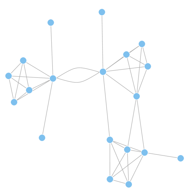
Figure 1: An undirected network with 19 nodes.

Leading eigenvector	Spectral clustering	Clique percolation	Classical NMF

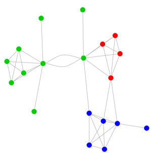
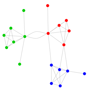
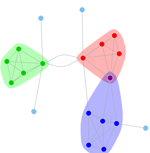
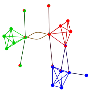
Figure 2: (Color online) Results using alternative community discovery methods.

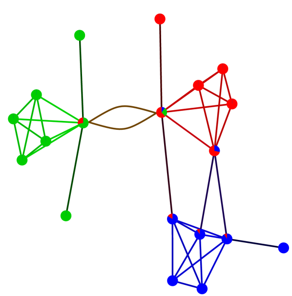
Figure 3: (Color online) Results from applying sparse NMF (Algo. 1) with $\lambda_{s}=5$. Nodes and edges are colored to denote the relative contribution of each community.

	Star Network	Ring Network
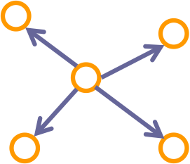
Adjacency Matrix	$\left[\begin{array}[]{ccccc}0&1&1&1&1\\ 0&0&0&0&0\\ 0&0&0&0&0\\ 0&0&0&0&0\\ 0&0&0&0&0\end{array}\right]$	$\left[\begin{array}[]{ccccc}0&1&0&0&1\\ 1&0&1&0&0\\ 0&1&0&1&0\\ 0&0&1&0&1\\ 1&0&0&1&0\end{array}\right]$
NMF $U,V$	$\left[\begin{array}[]{r}1.00\\ 0.00\\ 0.00\\ 0.00\\ 0.00\end{array}\right]\left[\begin{array}[]{r}0.00\\ 1.00\\ 1.00\\ 1.00\\ 1.00\end{array}\right]$	$\left[\begin{array}[]{r}0.89\\ 0.89\\ 0.89\\ 0.89\\ 0.89\end{array}\right]\left[\begin{array}[]{r}0.45\\ 0.45\\ 0.45\\ 0.45\\ 0.45\end{array}\right]$
Hub, Authority	$\left[\begin{array}[]{r}1.00\\ 0.00\\ 0.00\\ 0.00\\ 0.00\end{array}\right]\left[\begin{array}[]{r}0.00\\ 0.50\\ 0.50\\ 0.50\\ 0.50\end{array}\right]$	$\left[\begin{array}[]{r}0.45\\ 0.45\\ 0.45\\ 0.45\\ 0.45\end{array}\right]\left[\begin{array}[]{r}0.45\\ 0.45\\ 0.45\\ 0.45\\ 0.45\end{array}\right]$

Figure 4: Rank 1 NMF without penalization and Kleinberg’s authority/hub scores Kleinberg (1999).

II.1.2 Rank One Factorizations

We show in our experiments (Section IV) that a sequence of rank one matrix factorizations can be the basis for informative displays of time-varying node importance to connectivity. To provide some intuition as to why such a rank one factorization is informative, consider Fig. 4, which shows graph structures, corresponding NMFs, and Kleinberg’s authority and hub scores Kleinberg (1999). Authority and hub scores are computed by the leading eigenvector of $A^{T}A$ and $AA^{T}$, respectively. Subject to rescaling of the NMF estimates, the results are identical. In fact, by the Perron-Frobenius theorem (see Chapter 8 of Meyer (2000)), the rank one NMF solution is always a rescaled version of authority and hub scores. This provides a natural interpretation for the rank one NMF. For instance, the $U$ vector on the Star Network highlights the hub node. The $V$ vector show that all peripheral nodes are equal in terms of their authority (incoming connections), and that the central node has no incoming connections. NMF vectors of the Ring Network show each node with an equal score for incoming (authority) and outgoing (hub) connectivity. The fact that $U$ contains larger elements than $V$ is arbitrary. However, the assignment of equal values within $U$ and $V$ shows each node is equally important to interconnectivity.

III Model for Dynamic Networks

Given a time series of networks $\{\mathcal{G}_{t}=(V_{t},E_{t})\}_{t=1}^{T}$ with corresponding adjacency matrices $\{A_{t}\}_{t=1}^{T}$, the goal is to produce a sequence of low rank matrix factorizations $\{U_{t},V_{t}\}_{t=1}^{T}$.

To extend the factorization from the previous section to the temporal setting, we impose a smoothness constraint on the basis $U_{t}$. This constraint forces new community structure to be similar to previous time points. Since individual node time-series given by $U_{t}$ are visually smooth, time plots for each node become informative and provide an alternative to graph drawings for visualizing node dynamics. Moreover, time plots are static displays, which facilitate detailed analysis and avoid difficulties associated with animated layouts when given a large number of time points or nodes.

The objective function becomes

$$\min_{\{U_{t}\geq 0,V_{t}\geq 0\}_{t=1}^{T}} \sum_{t=1}^{T}||A_{t}-U_{t}V_{t}^{T}||_{F}^{2}$$

$${+}\>\lambda_{t}\sum_{t=1}^{T}\sum_{\tilde{t}=t-\frac{W}{2}}^{t+\frac{W}{2}}||U_{t}-U_{\tilde{t}}||_{F}^{2}$$

$${+}\>\lambda_{s}\sum_{t=1}^{T}\sum_{k=1}^{K}||V_{t,k}||_{1},$$

where $W$ is a small integer representing a time window. The parameters $\lambda_{t},\lambda_{s}\text{ and }W$ are set by the user to steer the analysis.

The interpretations of $U_{t},V_{t}$ extend naturally from the previous section, so that, for instance, $\sum_{k}(V_{t})_{kj}$ measures the importance of node $j$ (typically corresponding to incoming edges), and $(U_{t})_{ik}(V_{t})_{jk}/\sum_{k=1}^{K}(U_{t})_{ik}(V_{t})_{jk}$ to measure the relative contribution of each community to each $i,j$ edge. In principle, the edge decomposition can be used to assign nodes to communities as discussed in the last section. However, this approach can be unsatisfactory due to unstable community assignments. As alternative method is to assign communities in terms of $U_{t}$, which ensures the stability of the community structure through time. Specifically, measuring the contribution of node $i$ to each community with the relative magnitude of the $i$th element of each dimension of $U_{t}$, e.g., $(U_{t})_{ik}/\sum_{k=1}^{K}(U_{t})_{ik}$.

We can follow similar steps as in the last section to derive a gradient descent estimation algorithm. First, to enforce the non-negativity constraints, we consider the Lagrangian

$$L = \sum_{t=1}^{T}||A_{t}-U_{t}V_{t}^{T}||_{F}^{2}$$

$${+}\>\lambda_{t}\sum_{t=1}^{T}\sum_{\tilde{t}=t-\frac{W}{2}}^{t+\frac{W}{2}}||U_{t}-U_{\tilde{t}}||_{F}^{2}$$

$${+}\>\lambda_{s}\sum_{t=1}^{T}\sum_{i=1}^{n}\sum_{j=1}^{K}|V_{t}(i,j)|$$

$${+}\>\sum_{t=1}^{T}Tr(\Phi_{t}U_{t}^{T})+\sum_{t=1}^{T}Tr(\Psi_{t}V_{t}^{T}),$$

where $\Phi_{t},\Psi_{t}$ are Lagrange multipliers.

The following KKT optimality conditions are obtained by setting $\frac{\partial L}{\partial U_{t}}=\frac{\partial L}{\partial V_{t}}=0$.

$$\Phi_{t} = -2A_{t}V_{t}+2U_{t}V_{t}^{T}V_{t}-2\lambda_{t}\sum_{\tilde{t}=t-\frac{W}{2}}^{t-1}U_{\tilde{t}}$$

$${-}\>2\lambda_{t}\sum_{\tilde{t}=t+1}^{t+\frac{W}{2}}U_{\tilde{t}}+2W\lambda_{t}U_{t}$$

$$\Psi_{t} = -2A_{t}^{T}U_{t}+2V_{t}U_{t}^{T}U_{t}+2\lambda_{s}.$$ (12)

Then, the KKT complimentary slackness conditions yield

$$0 = (-2A_{t}V_{t}+2U_{t}V_{t}^{T}V_{t}-2\lambda_{t}\sum_{\tilde{t}=t-\frac{W}{2}}^{t-1}U_{\tilde{t}})_{ij}(U_{t})_{ij}$$

$${+}\>(-2\lambda_{t}\sum_{\tilde{t}=t+1}^{t+\frac{W}{2}}U_{\tilde{t}}+2W\lambda_{t}U_{t})_{ij}(U_{t})_{ij}$$

$$0 = (-2A_{t}^{T}U_{t}+2V_{t}U_{t}^{T}U_{t}+2\lambda_{s})_{ij}(V_{t})_{ij},$$ (14)

which after some algebra leads to the algorithm provided in Algo. 2. The theoretical properties are also the same as in the previous section. Most notably, the estimates of $U_{t}$ and $V_{t}$ will improve at each iteration with respect to Eq. III.

1:Set constants $\lambda_{t},\lambda_{s},W$.

2:Initialize $\{U_{t}\},\{V_{t}\}$ as dense, positive random matrices.

3:repeat

4:   for t=1..T do

5:      Set

6:$(U_{t})_{ij}\leftarrow(U_{t})_{ij}\frac{(A_{t}V_{t}+\lambda_{t}\sum_{\tilde{t}=t-\frac{W}{2}}^{t-1}U_{\tilde{t}}+\lambda_{t}\sum_{\tilde{t}=t+1}^{t+\frac{W}{2}}U_{\tilde{t}})_{ij}}{(U_{t}V_{t}^{T}V_{t}+W\lambda_{t}U_{t})_{ij}}$.

7:      Set

$$(V_{t})_{ij}\leftarrow(V_{t})_{ij}\frac{(A_{t}^{T}U_{t})_{ij}}{(V_{t}U_{t}^{T}U_{t})_{ij}+\lambda_{s}}.$$

8:   end for

9:until Convergence

List of Algorithms 2 NMF with temporal and sparsity penalties

III.1 Parameter Selection

We briefly discuss the important practical matter of choosing $K$, the inner rank of the matrix factorization.

For the goal of clustering, the rank should be equal to the number of underlying groups. The rank can be ascertained by examining the accuracy of the reconstruction as a function of rank. However, this tends to rely on subjective judgments and overfit the given data. Cross validation based approaches are theoretically preferable and follow the same intuition.

The idea behind cross validation is to use random subsets of the data from each data slice to fit the model, and another subset from each data slice to assess accuracy. Different values of $K$ are then cycled over and the one that corresponds to the lowest test error is chosen.

Due to the data structure, we employ two-dimensional cross validation. Two-dimensional refers to the selection of submatrices for our training and test data. Special care is taken to ensure that the same rows and columns are held out of every data slice, and the dimensions of the training and test sets are identical.

The hold out pattern divides the rows into $k$ groups, the columns into $l$ groups, then uses the corresponding $kl$ submatrices to fit and test the model. In each submatrix, the given row and column group identifies a held out submatrix that is used as test data, while the remaining cells are used for training. The algorithm is shown in Algo. 3. The notation in the algorithm uses $\mathcal{I}_{l}$ and $\mathcal{I}_{J}$ as index sets to identify submatrices in the each data matrix.

1:Form row holdout set: $\mathcal{I}_{l}\subset\{1,..,n\}$

2:Form column holdout set: $\mathcal{I}_{J}=\subset\{1,..,n\}$

3:Set

$$(\tilde{U}_{t},\tilde{V}_{t})=\operatorname*{arg\,min}_{U_{t},V_{t}\geq 0}\sum_{t}||(A_{t})_{-\mathcal{I}_{l},-\mathcal{I}_{J}}-U_{t}V_{t}^{T}||_{F}^{2}$$

4:Set

$$\breve{U_{t}}=\operatorname*{arg\,min}_{U_{t}\geq 0}\sum_{t}||(A_{t})_{\mathcal{I}_{l},-\mathcal{I}_{J}}-U_{t}\tilde{V}_{t}^{T}||_{F}^{2}$$

5:Set

$$\breve{V}_{t}=\operatorname*{arg\,min}_{V_{t}\geq 0}\sum_{t}||(A_{t})_{-\mathcal{I}_{l},\mathcal{I}_{J}}-\tilde{U}_{t}V_{t}^{T}||_{F}^{2}$$

6:Set

$$\hat{(A_{t})}_{\mathcal{I}_{l},\mathcal{I}_{J}}=\breve{U}_{t}\breve{V}_{t}^{T}$$

7:Compute Test error

$$\text{Test Error}=\sum_{t}||(A_{t})_{\mathcal{I}_{l},\mathcal{I}_{J}}-\hat{(A_{t})}_{\mathcal{I}_{l},\mathcal{I}_{J}}||_{F}^{2}$$

List of Algorithms 3 Cross-validation for choosing the number of communities (rank)

We then cycle over different values of $K$ to choose the one that minimizes average test error. Fig. 5 shows that this procedure correctly identifies 3 communities for the toy example. Consistency results are developed in Perry and Owen (2009) to provide theoretical foundations for this approach.

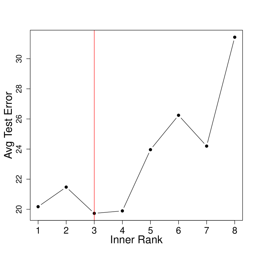
Figure 5: Cross validation indicates 3 communities (rank 3) features the lowest average test error for the toy example.

In principle the cross validation procedure can be used to select the penalties $\lambda_{t},\lambda_{s}$ and the time window $W$. However, considering the scale of many modern network datasets, this would require too much computing time. Instead we typically choose the penalties by hand to emphasize readability and interpretability of the results, keeping in mind that if either penalty is set too large then the estimation results in degenerate solutions. For instance, the algorithm suffers from numerical instabilities when $\lambda_{s}$ is too large, since all $V_{t}$ elements are zero. If $\lambda_{t}$ is set to an extremely large number, then $U_{t}$ will be approximately constant for all time periods, so the effective model is $A_{t}\approx UV_{t}^{T}$, e.g., the community structure is fixed for all observations.

The parameter, $W$, controls the number of neighboring time steps to locally average. Larger values of $W$ mean that the model has more memory so it incorporates more time points for estimation. This risks missing sharper changes in the data and only detecting the most persistent patterns. On the other hand, small values of $W$ make the fitting more sensitive to sharp changes, but increase short term fluctuations due to smaller number of observations. We set $W=2$ (looking one time period ahead and before) for all presented experiments. Larger values could be used in very noisy settings to further smooth results.

IV Experiments

In this section we test the model on both synthetic and real-world examples. The synthetic networks allow us to validate the model’s ability to highlight known community structure and node evolution, while the real examples exhibit the model’s performance under practical conditions.

IV.1 Synthetic Networks

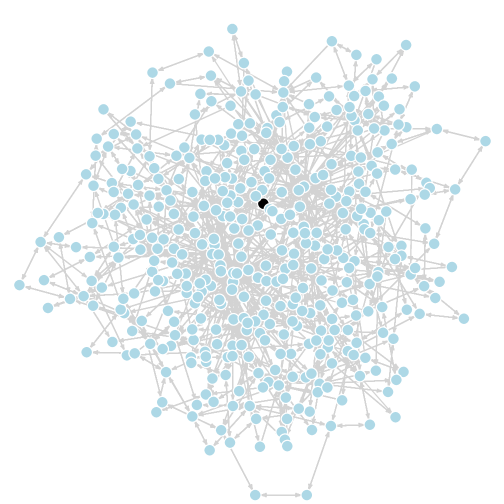
Figure 6: The cell phone network from a day using a force directed layout algorithm in igraph. Node 200 is colored black.

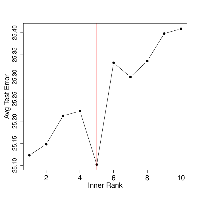
Figure 7: Choosing $K$ for the Catalano communications network. The left panel shows the average residual sum of squares, and the right panel shows the average test error obtained via cross validation ($5\times 5$ fold) for different the approximation ranks. Cross validation indicates that 5 communities is optimal.

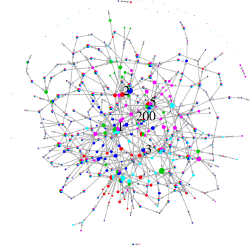
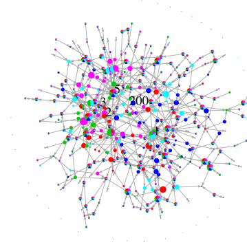
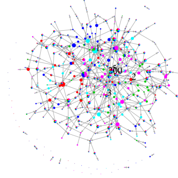
Day 5 Day 6 Day 7 Raw Fitted

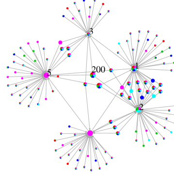
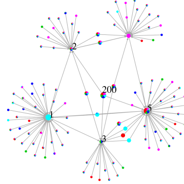
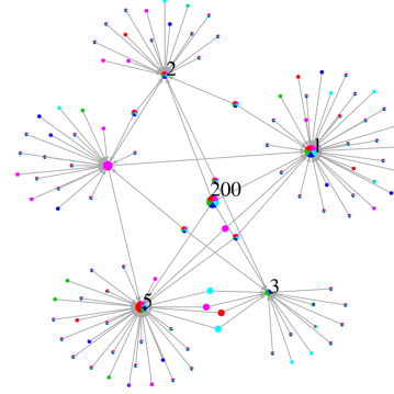
Figure 8: (Color online) The raw (top row) and filtered Catalano networks (bottom row) colored by the $U_{t}$ community structure. A force directed layout in igraph was used to create this embedding. Nodes are colored by soft partitioning via the penalized NMF.

IV.1.1 Catalano Communication Network

The first example utilizes the Catalano social network, which was part of the Visual Analytics Science and Technology (VAST) 2008 challenge vas (2008). The synthetic data consists of 400 unique cell phone IDs over a ten day period. Altogether, there are 9834 phone records with the following fields: calling phone identifier, receiving phone identifier, date, time of day, call duration, and cell tower closest to the call origin. The purpose of the challenge was to characterize the social structure over time for a fictitious, controversial socio-political movement. In particular, the challenge requires identifying five key individuals that organize activities and communications for the network; a hint was given to challenge participants that node 200 is one of the persons of interest.

We use the first seven days of data to illustrate our methodology, since there is a strong change in the connection patterns from day 8-10 for node 200 (see vas (2008); Shaverdian et al. (2009) and references therein). Directed networks are constructed daily by drawing an edge from the caller to the receiver. Fig. 6 shows an example of one day’s network. The graph is too cluttered to visually identify leaders of the network or get a sense of the network structure.

We fit a sequence of rank 5 NMFs, as identified in Fig. 7 through cross validation, with a large temporal penalty to highlight the most persistent interactions. Fig. 8 shows two sets of graph drawings for three days (due to space limitations), with the nodes colored according to their community membership. The first row shows the graph constructed directly from the data, while the second row shows graph drawings of the fitted model $\hat{A}=U_{t}V_{t}^{T}$. The clustering results applied to the raw data are not interpretable, as the data is simply too cluttered. However, the persons of interest and the hierarchical structure of the communication network are clearly shown when considering the fitted networks. One can visually identify that node $200$ consistently relays information to his neighbors (1,2,3,5), who disseminate information to their respective subordinates. We can also see that nodes higher up on the organizational hierarchy tend to belong to multiple communities, presumably since they disseminate information to different groups of subordinates.

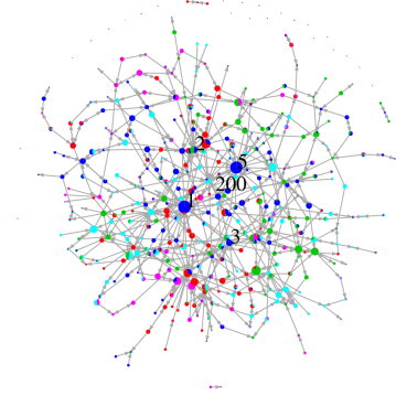
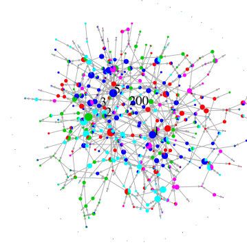
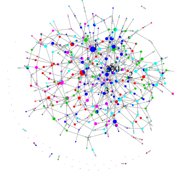
Day 5 Day 6 Day 7 Raw Fitted

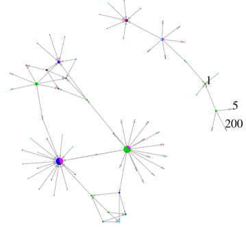
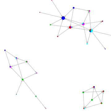
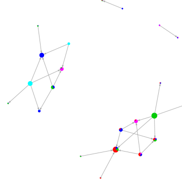
Figure 9: (Color online) Results of applying the Facetnet factorization Lin et al. (2008) with a prior weight of $\lambda=0.8$. The raw (top row) and filtered Catalano networks (bottom row) colored by the Facetnet factorization.

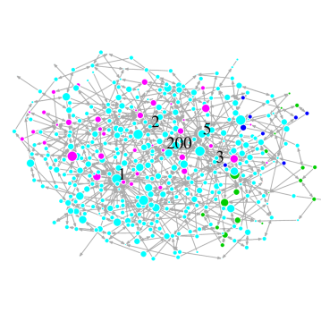
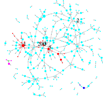
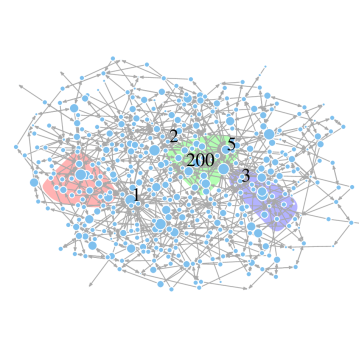
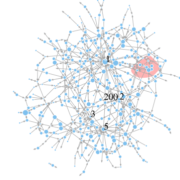
Threshold=2 Threshold=3 Threshold=4 Spectral Clustering Clique Percolation No Communities Detected

Figure 10: (Color online) The first and second rows apply static clustering methods to the collapsed data (averaging over time). All alternative methods struggle to identify the key individuals or hierarchical organizational structure.

Fig. 9 shows the results of applying Facetnet Lin et al. (2008), an alternative NMF methodology for dynamic overlapping community detection. Facetnet applies an underlying model with less flexibility resulting in poor reconstructions of the data, as seen in the fitted networks. We also collapse the data into a single network snapshot in order to apply static clustering algorithms. First, an edge is kept only if it was observed more than Threshold days. Then, spectral clustering and clique percolation are applied to the resultant network snapshot. All alternative methods struggle, as the data is too ‘hairball’ like. On the other hand, the fitted penalized NMF model provides a unified framework to filter the network and visualize community structure. VAST never officially released correct answers for the challenge. However, our analysis closely matches winning entries Shen and Ma (2008); Ye et al. (2009); Shaverdian et al. (2009). Treating the conclusions of the entries as ground truth, we have provided a simple workflow that uncovers patterns in the data that are not directly obtainable with traditional methods.

IV.1.2 Preferential Attachment Process

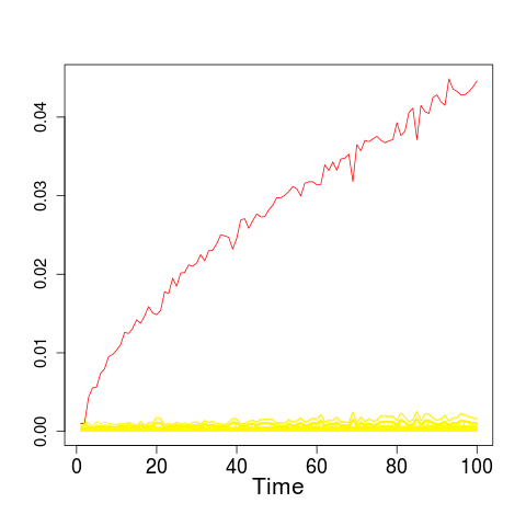
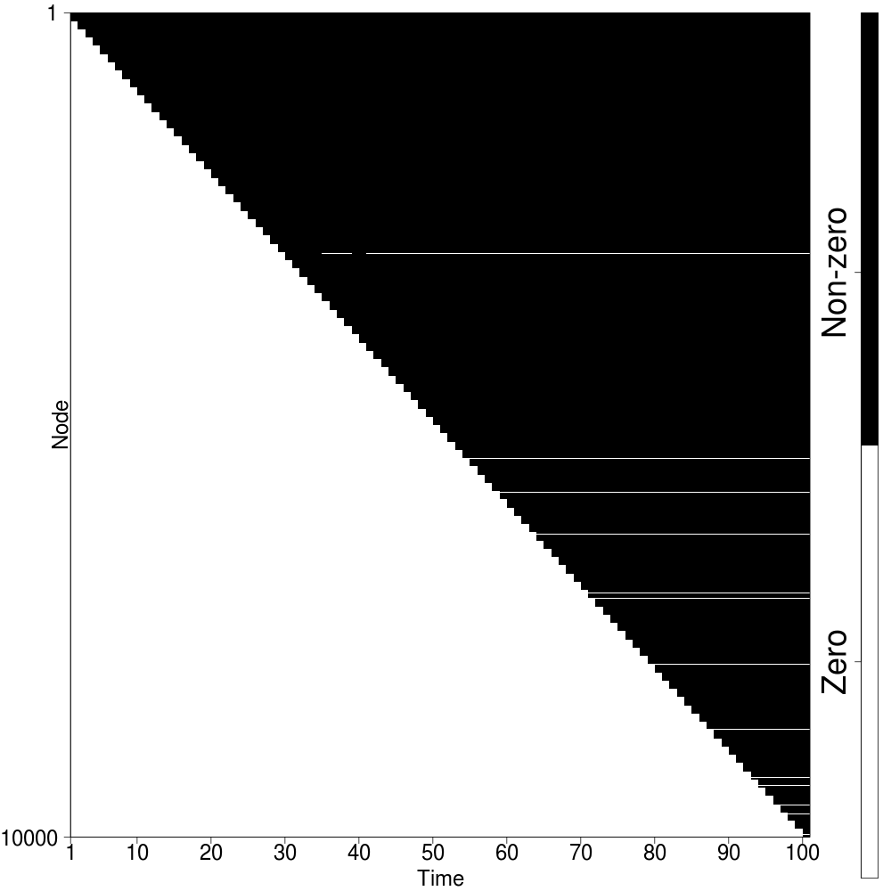
(a) No penalties

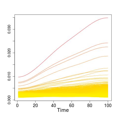
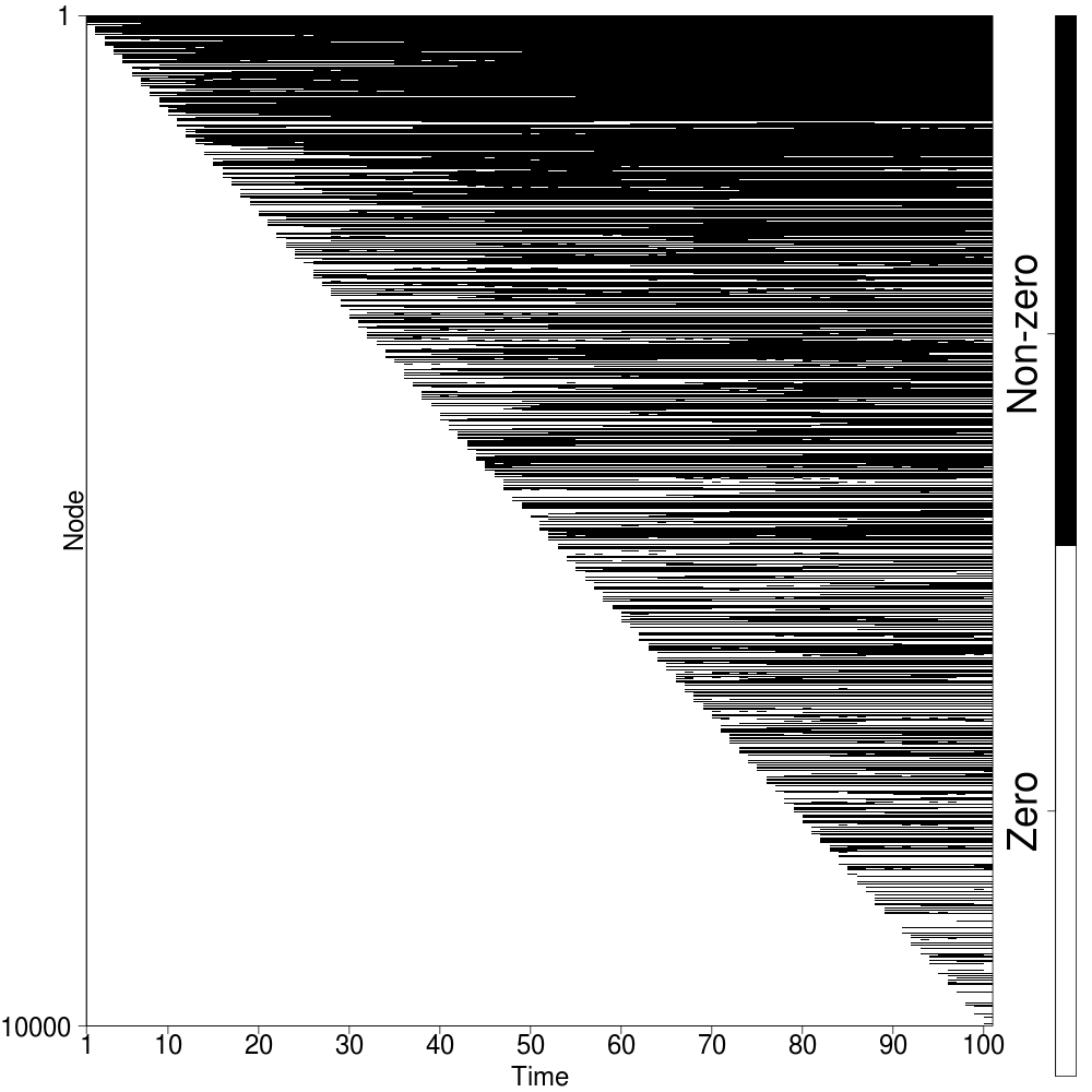
(b) $\lambda_{t}=50,\lambda_{s}=5$

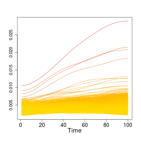
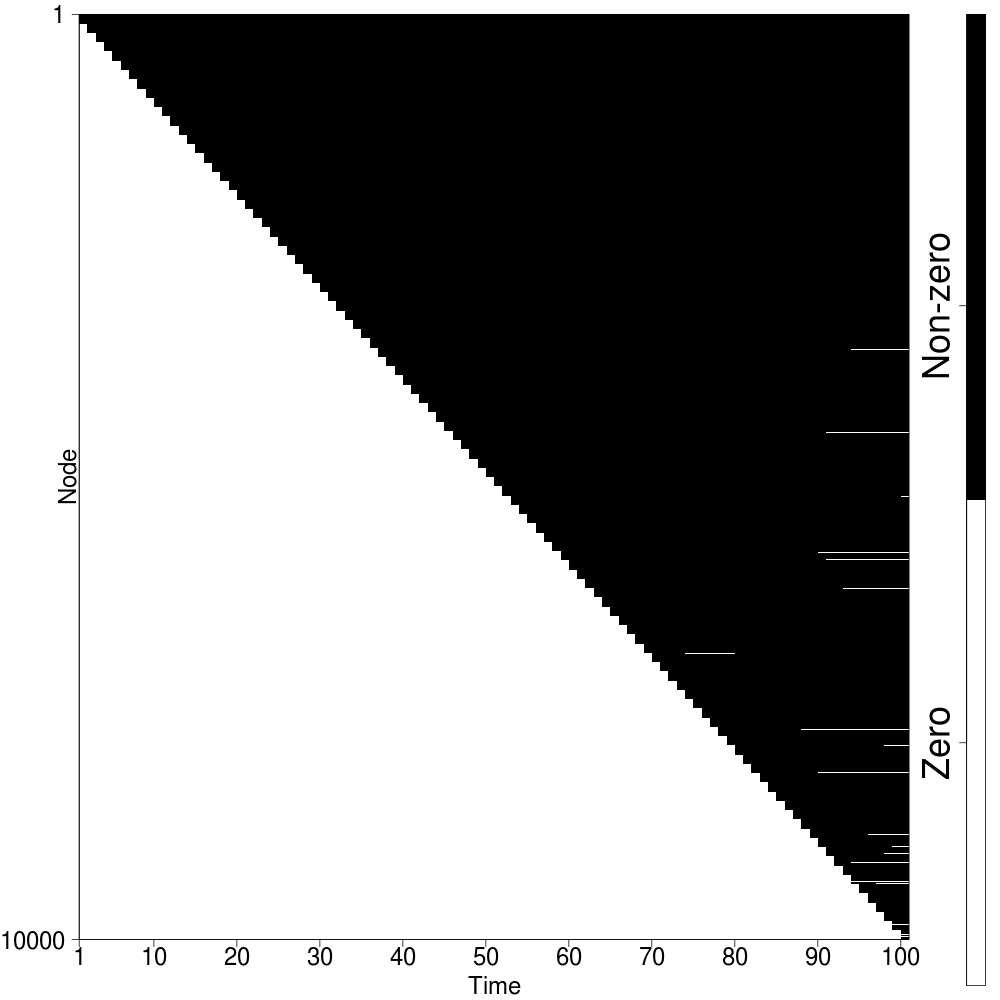
(c) $\lambda_{t}=100,\lambda_{s}=5$

Figure 11: (Color online) Fitted values for $U$ and $V$ over time for the preferential attachment simulation. The left column shows a time plot of $U_{t}$ over different parameter values. Each line corresponds to a node on the graph. The right column identifies the nonzero elements of $V_{t}$. Each row corresponds to a node on the graph and time varies along the horizontal axis.

In this simulation, nodes attach according to a preferential attachment model Newman et al. (2006); Barabási and Albert (1999) until $10000$ nodes have ’attached’ to the embedding. We observe this growing process at 100 uniformly spaced time points. Thus, at each time point 100 new nodes attach to the graph. We use source code from a networks MATLAB toolbox Bounova (2011) that generates preferential attachment graphs according to the standard model.

In the preferential attachment model, $\Pi(i)$, which represents the probability that a new node connects to node $i$, depends on node $i$’s degree. Specifically, we have

$$\Pi(i)\propto d_{i}$$ (15)

where $d_{i}$ is the degree of the $ith$ node. This generating framework leads to networks whose asymptotic degree distribution follows a power-law distribution with parameter $\gamma=3$. Graphs with heavy-tailed degree distributions are commonly observed in a variety of areas, such as the Internet, protein interactions, citation networks, among others Clauset et al. (2009).

In practice, an analyst would not know that the data comes from a preferential attachment process. In which case, an exploratory analysis may include inspecting the network sequence on a set of standard metrics (degree, transitivity, centrality, etc.), graph drawings, as well as community detection approaches. We believe that a sequence of one-dimensional ($K=1$) penalized NMFs can serve as the basis for a complimentary exploratory tool that helps uncover different connectivity patterns and evolution in the data. In particular, due to the smoothness penalty, time plots in $U_{t}$ for each node become useful for uncovering the number and types of node evolutions in the data. Similarly, heatmaps or displays of the sparsity pattern of $V_{t}$ are useful to identify when nodes/groups become significantly active.

Since preferential attachment networks have been extensively studied, we show only the NMF-based displays. Fig. 11 shows important (hub) nodes that distinct trajectories that indicate their increasing importance to the network over time. The $V_{t}$ sparsity features a pseudo-upper triangular form. This corresponds to the node attachment order and reflects that nodes permanently attach after connecting to the network. Such displays can be created quickly and can help the process of identifying interesting nodes, formulating research questions, and so on.

Also shown in Fig. 11 is that penalization is important to the usefulness and interpretability of the displays. For instance, without a temporal penalty, the time plots emphasize only the highest degree node. With appropriate penalties, an analyst can visually identify the different hub nodes.

IV.2 Real Networks

IV.2.1 arXiv Citations

We investigate a time series of citation networks provided as part of the 2003 KDD Cup Gehrke et al. (2003). The graphs are from the e-print service arXiv for the ‘high energy physics theory’ section.

The data covers papers in the period from October 1993 to December 2002, and is organized into monthly networks. In particular, if paper $i$ cites paper $j$, then the graph contains a directed edge from $i$ to $j$. Any citations to or from papers outside the dataset are not included. Following convention, edges are aggregated, that is, the citation graph for a given month will contain all citations from the beginning of the data up to, and including, the current month. Altogether, there are $22750$ nodes (papers) with $176602$ edges (references) over $112$ months.

Jan 1995 Jan 1998 Jan 2000

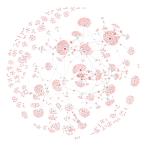
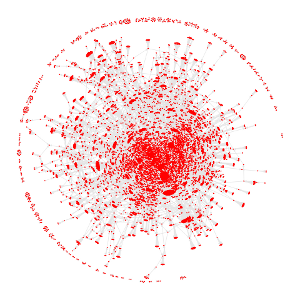
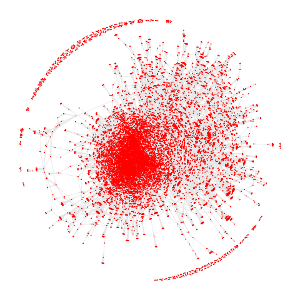
Figure 12: Graph layouts of the arXiv data at three different time points. Due to the size of the networks, it quickly becomes difficult to discern paper (node) properties.

As a first step towards investigating the data, we draw the network at different points in time in Fig. 12. Even when considering a single time point, it quickly becomes difficult to discern paper (node) properties due to the large network size. Thus, the data requires network statistics and other methods to extract structure and infer dynamics in the network sequence. Network statistics, shown in Fig. 13, provide some additional insight. There is a noticeable increase in network growth around the year 2000, which is commonly attributed to papers that reference other works before the start of the observation period (see Leskovec et al. (2005)). As we move away from the beginning of the data, papers primarily reference other papers belonging to the data set. Additional statistical properties of the data were discussed in Leskovec et al. (2005), which found that the networks feature decreasing diameter over time and heavy-tailed degree distributions.

Figure 13: (Color online) ArXiv network statistics over time. The kink near near January 2000 indicates sudden, rapid growth. The top-left plot is on a log-log scale.

To visualize how nodes in the network evolved, Fig. 14 displays results from the matrix factorization model using a sequence of one-dimensional approximations ($K=1$). The adjacency matrix is constructed so that $U_{t}$ scores nodes by their importance to the average incoming connections, and $(U_{t})_{1j}$ measures the time-varying authority of paper $j$. $V_{t}$ yields similar scores based on outgoing connections. As observed with the preferential attachment experiment, the paper trajectories are smoothed effectively and important dynamics are highlighted by employing penalties. Specifically, there are two important periods in the data. The first period covers 1996-1999, and featured papers mostly on an extension of string theory called M-theory. M-theory was first proposed in 1995 and led to new research in theoretical physics. A number of scientists, including Witten, Sen and Polchinski, were important to the historical development of the theory, and as seen in Tables 1 and Table 2, our NMF approach identifies these important authors and their works. From 1999-2000 the rate of citations to these papers tended to decrease, while focus shifted to other topics and subfields that M-theory gave rise to. These citation patterns are reflected in the bold and dashed trajectories in Fig. 14. The displays of $V_{t}$ sparsity show that papers do not appear uniformly throughout time. Instead as other network statistics show, papers ‘attach’ at a faster rate around year 2000.

No Penalty	$\lambda_{s}=1$	$\lambda_{s}=5$	$\lambda_{s}=10$

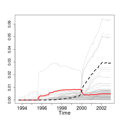
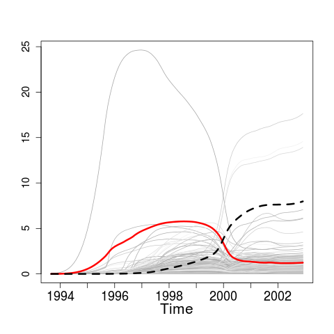
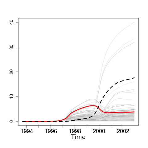
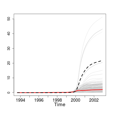
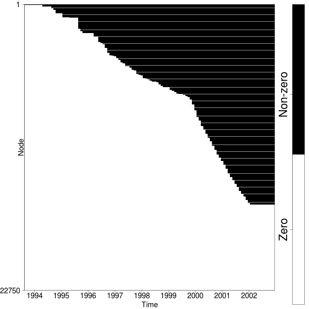
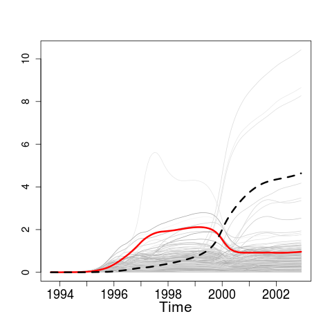
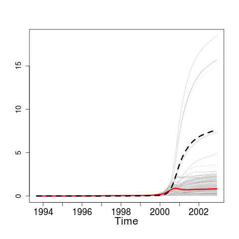
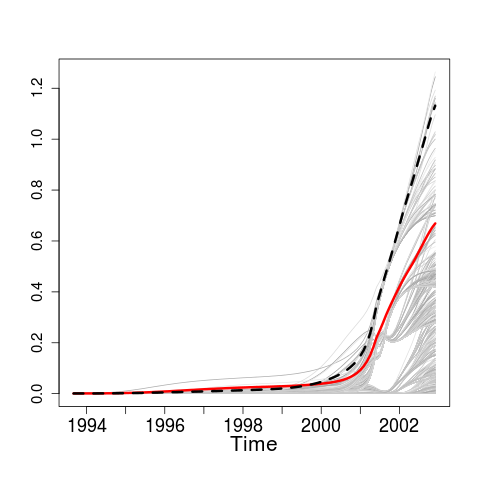
Figure 14: (Color online) Fitted values for $U_{t}$ and $V_{t}$ for the arXiv data with $\lambda_{t}=5$. Each light gray line corresponds to a paper (node) on the graph. The bold lines show the average of the 10 papers with highest average $\hat{U}$ from 1996-1999, and 2000 onwards (dashed). Each row in the heatmaps corresponds to a paper and time varies along the horizontal axis.

We provide comparisons with the alternative methodologies utilized in Leicht et al. (2007) to investigate dynamic citation network from the US Supreme Court. First, we apply the leading eigenvector modularity-based method for community discovery Newman (2006) to the fully formed citation network ($t=112$). The second alternative methodology is a mixture model in Leicht et al. (2007) to extract groups of papers according to their common temporal citation profiles.

The left panel of Fig. 15 shows the degree of each paper over time, colored by the leading eigenvector community assignments. The optimal number of groups is over two hundred. There are four large groups of papers, with the other groups containing only a handful of papers. This approach does not utilize the temporal profile of each paper, and as a consequence the groups are interpretable from a static connectivity point of view only.

The right panel of Fig. 15 shows reasonable time-profiles from the mixture model. One group grows slowly from the beginning of the observational period, while the other group experiences rapid growth starting around the year 2000. These results compliment the NMF-based Fig. 14, and together provide a robust methodology to identify important papers, as well as characterize the data in terms of the number and types of different nodes/groups in the data.

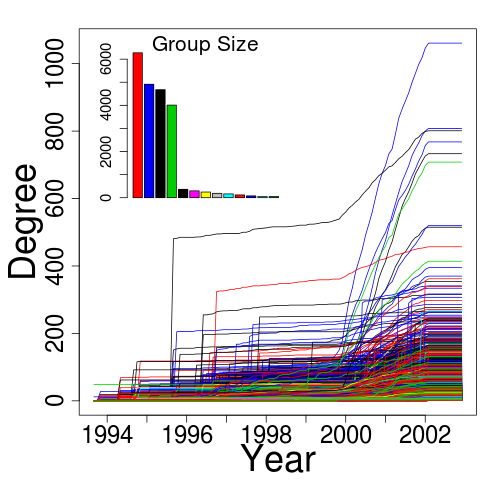
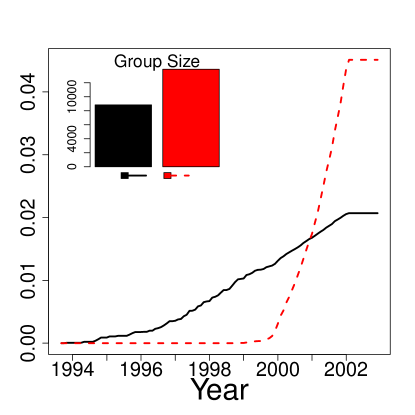
Figure 15: The left panel shows the degree of each node over all time points, colored by the leading eigenvector groupings. The right panel shows time-profiles for each group based on the mixture model of Leicht et al. (2007).

Table 1: The top 10 papers with highest average $\hat{U}$ from 1996-1999. # Citations counts all references to the work, including by papers outside of our data. These counts obtained via Google.

Title Authors In-Degree Out-Degree # Citations (Google) Heterotic and Type I String Dynamics from Eleven Dimensions Horava and Witten 783 18 2334 Five-branes And $M$-Theory On An Orbifold Witten 169 15 251 Type IIB Superstrings, BPS Monopoles, And Three- Hanany and Witten 437 20 844 Dimensional Gauge Dynamics D-Branes and Topological Field Theories Bershadsky, et al. 271 15 463 Lectures on Superstring and M Theory Dualities Schwarz 247 68 534 D-Strings on D-Manifolds Bershadsky et al. 172 22 247 String Theory Dynamics In Various Dimensions Witten 263 0 2263 Branes, Fluxes and Duality in M(atrix)-Theory Ganor, et al. 184 16 243 Dirichlet-Branes and Ramond-Ramond Charges Polchinski 370 0 2592 Matrix Description of M-theory on $T^{5}$ and $T^{5}/Z_{2}$ Seiberg 208 30 353

Table 2: The top 10 papers with highest average $\hat{U}$ from 2000 onwards.

Title Authors In-Degree Out-Degree # Citations (Google) The Large N Limit of Superconformal Field Theories and Supergravity Maldacena 1059 2 10697 Anti De Sitter Space And Holography Witten 766 2 6956 Gauge Theory Correlators from Non-Critical String Theory Gubser et al. 708 0 6004 String Theory and Noncommutative Geometry Seiberg and Witten 796 12 3833 Large N Field Theories, String Theory and Gravity Aharony et a. 446 74 3354 An Alternative to Compactification Randall and Sundrum 733 0 5693 Noncommutative Geometry and Matrix Theory: Compactification on Tori Connes et al. 512 3 1810 M Theory As A Matrix Model: A Conjecture Banks et al. 414 0 2460 D-branes and the Noncommutative Torus Douglas and Hull 296 2 866 Dirichlet-Branes and Ramond-Ramond Charges Polchinski 370 0 2592

IV.2.2 Global Trade Flows

In this example, we analyze annual bilateral trade flows between 164 countries from 1980-1997 Feenstra et al. (2004). Thus, we observe a dynamic, weighted graph at 18 time points, where each directional edge denotes the total value of exports from one country to another. Since trade flows can differ in size by orders of magnitude, we work with trade values that are expressed in log dollars.

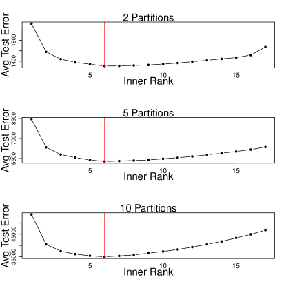
Figure 16: Choosing $K$ for World Trade Data. The left panel shows the average residual sum of squares. The right panel shows the average test error obtained via cross validation for different number of partitions. Cross validation consistently indicates 6 communities ($K=6$) as optimal.

We fit a sequence of rank 6 NMFs, as identified in Fig. 16 through cross validation, and display the network based on fitted trade flows ($\hat{A}_{t}=U_{t}V_{t}^{T}$) in Fig. 17. We show only three years (1980, 1990, 1997) due to space constraints.

All countries belong to more than one community, which reflects the interconnected nature of the global economy. However, there are countries, primarily from Africa and Central America, that are dominated by a single community or belong to only a subset of the six communities. For instance, in 1997, Ecuador, Venezuela and Panama only connect with the USA and hence, belong mostly to the green community.

There are also interesting findings that correspond with historical events. For instance, in 1980 there is a strong community (circled in the figure) consisting of countries aligned with the former USSR, which acted as a hub. However by 1990, this community has dissolved, and is reflected in the edge and node colorings of these countries (more diversified trading relationships). In 1990, we also see the emergence of the so-called ’Asian miracles’, countries in Asia that experienced persistent and rapid economic growth in the 1990’s Stiglitz (1996); Nelson and Pack (1998). These countries move closer to the center of the trading network with membership in all communities.

1980	1990	1997

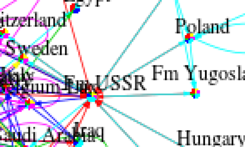
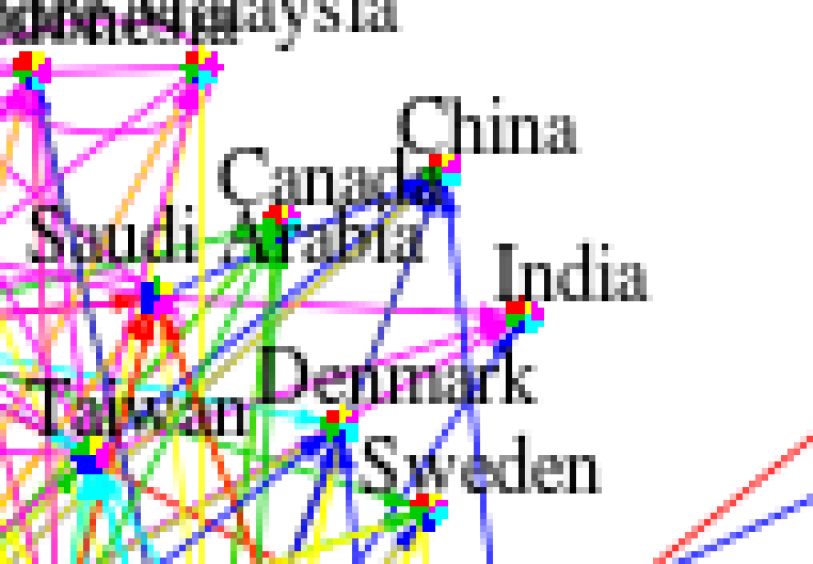
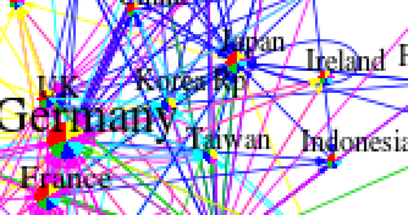
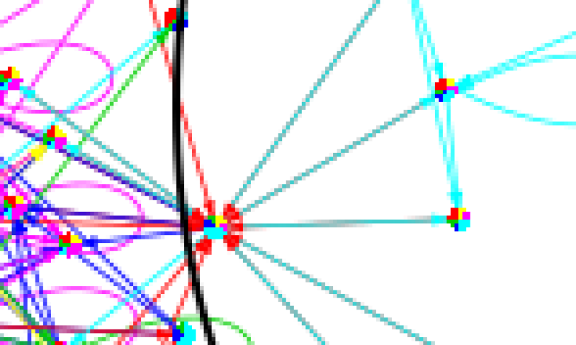
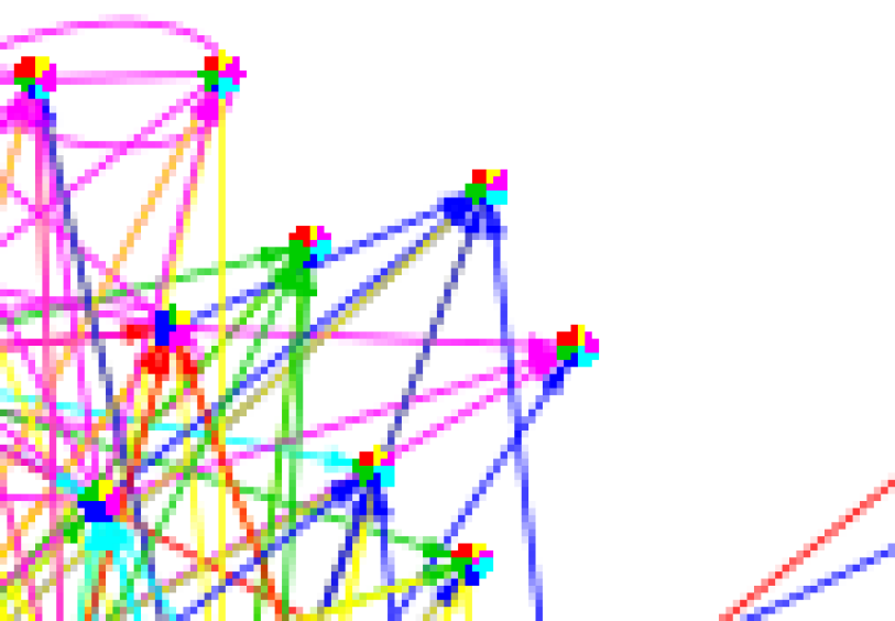
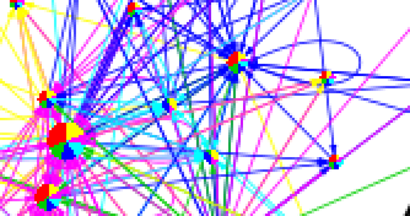
Figure 17: (Color online) World trade networks over time, where countries are colored corresponding to their membership in 6 communities. Edges are colored by the community with largest relative contribution. The bottom row shows the same network drawing without labels.

V Discussion

The main idea behind the approach presented in this paper is to abstract the network sequence to a sequence of lower dimensional spaces using matrix factorizations for visual exploration, community detection and structural discovery. Next, we highlight some of the strengths and weaknesses of this approach.

V.1 Strengths

An important benefit is the versatility and scalability of matrix factorization model. Table 3 shows runtimes for all experiments. The computational cost is low enough to use in combination with other analysis and visualization tools. Moreover, the penalized NMF approach is compatible with both binary and weighted networks.

Table 3: Average runtimes for the penalized NMF with temporal and sparsity penalties. The computational time scales approximately linearly with the number of time points and nodes.

Data Nodes Time Points Runtime (seconds) Catalano 400 7 0.29 World Trade 164 18 0.51 Preferential Attachment 10000 100 39.45 arXiv Citations 22750 112 60.64

Using the model as a basis for an exploratory visual tool can help users uncover different connectivity patterns and evolution in the data. The estimates of $U_{t}$ and $V_{t}$ can be used for community discovery or a ranking of nodes based on their importance to connectivity for subsequent analysis. Displays of the factorizations can provide a sense of the data complexity, namely the types and number of node evolutions.

V.2 Weaknesses

The optimal choice of tuning parameters ($\lambda_{t},\lambda_{s}$) is dependent on perception and how the edge weights are scaled. This can limit the benefits of the proposed approach when given multiple datasets.

Time plots and heatmaps to visualize each factor yield limited information about global topology. For example, one can see from Figs. 11 and 14 that there are dominant nodes, but in principle, there could be many topologies that feature dominant nodes. One cannot say for sure without additional analysis that the networks follow a particular connectivity model. Thus, combining the matrix factorization model in this article with existing analysis and visualization tools can provide a more comprehensive analysis of the data.

V.3 Future Work

An important area of exploration would be to systematically compare penalized versions of NMF and SVD. In this work we chose to focus on NMF, since we find the corresponding displays preferable in terms of interpretability. This is generally consistent with existing literature on matrix factorization. However, SVD of graph related matrices have deep connections to classical spectral layout and problems in community detection. There may be classes of graph topologies and particular visualization goals under which SVD is preferable.

There could also be other types and combinations of penalties that are useful in visualization and detection of graph structure. For instance, depending on the precise meaning of a directional edge, one may desire both smoothness and sparsity for $U_{t}$, $V_{t}$ or both factors. Nonetheless, variants on the penalty structure will result in models that require roughly the same computational costs. Thus, this work provides evidence that penalized matrix factorization models are promising for structural and functional discovery in dynamic networks.

References

- Fienberg (2012) S. E. Fienberg, Journal of Computational and Graphical Statistics 21, 825 (2012).
- Goldenberg et al. (2009) A. Goldenberg, A. X. Zheng, S. E. Fienberg, and E. M. Airoldi, ArXiv e-prints (2009), arXiv:0912.5410 [stat.ME] .
- Girvan and Newman (2002) M. Girvan and M. E. J. Newman, Proceedings of the National Academy of Science 99, 7821 (2002), arXiv:cond-mat/0112110 .
- Ball et al. (2011) B. Ball, B. Karrer, and M. E. J. Newman, Phys. Rev. E 84, 036103 (2011), arXiv:1104.3590 .
- Leicht et al. (2007) E. A. Leicht, G. Clarkson, K. Shedden, and M. E. Newman, The European Physical Journal B 59, 75 (2007).
- Sarkar and Moore (2006) P. Sarkar and A. Moore, in Advances in Neural Information Processing Systems 18, edited by Y. Weiss, B. Schölkopf, and J. Platt (MIT Press, Cambridge, MA, 2006) pp. 1145–1152.
- Hoff et al. (2002) P. D. Hoff, A. E. Raftery, and M. S. Handcock, Journal of the American Statistical Association 97, 1090 (2002).
- Sun et al. (2007) J. Sun, C. Faloutsos, S. Papadimitriou, and P. S. Yu, in Proceedings of the 13th ACM SIGKDD international conference on Knowledge discovery and data mining, KDD ’07 (ACM, New York, NY, USA, 2007) pp. 687–696.
- Kolar et al. (2010) M. Kolar, L. Song, A. Ahmed, and E. P. Xing, Annals of Applied Statistics 4, 94 (2010), ”arXiv”:0812.5087 .
- Richard et al. (2012) E. Richard, P.-A. Savalle, and N. Vayatis, ArXiv e-prints (2012), arXiv:1205.1406 [stat.ML] .
- Asur et al. (2009) S. Asur, S. Parthasarathy, and D. Ucar, ACM Trans. Knowl. Discov. Data 3, 16:1 (2009).
- Raginsky et al. (2012) M. Raginsky, R. Willett, C. Horn, J. Silva, and R. Marcia, Information Theory, IEEE Transactions on 58, 5544 (2012), 0911.2904 .
- Psorakis et al. (2011) I. Psorakis, S. Roberts, M. Ebden, and B. Sheldon, Phys. Rev. E 83, 066114 (2011).
- Wang et al. (2011) F. Wang, T. Li, X. Wang, S. Zhu, and C. Ding, Data Mining and Knowledge Discovery 22, 493 (2011).
- Fortunato and Barthélemy (2007) S. Fortunato and M. Barthélemy, Proceedings of the National Academy of Sciences 104, 36 (2007), arXiv:physics/0607100 .
- Frishman and Tal (2008) Y. Frishman and A. Tal, Visualization and Computer Graphics, IEEE Transactions on 14, 727 (2008).
- Archambault et al. (2011) D. Archambault, H. Purchase, and B. Pinaud, Visualization and Computer Graphics, IEEE Transactions on 17, 539 (2011).
- Ghani et al. (2012) S. Ghani, N. Elmqvist, and J.-S. Yi, Computer Graphics Forum (Proc. EuroViz 2012) 31, 1205 (2012).
- von Landserber et al. (2010) T. von Landserber, A. Kuijper, T. Schreck, J. Kohlhammer, J.-J. van Wijk, and D.-W. Fellner, EuroGraphics state of the art reports (2010).
- von Landesberger et al. (2011) T. von Landesberger, A. Kuijper, T. Schreck, J. Kohlhammer, J. van Wijk, J.-D. Fekete, and D. Fellner, Computer Graphics Forum 30, 1719 (2011).
- Yi et al. (2010) J. S. Yi, N. Elmqvist, and S. Lee, International Journal of Human-Computer Interaction 26, 1031 (2010).
- Hastie et al. (2001) T. Hastie, R. Tibshirani, and J. H. Friedman, The elements of statistical learning: data mining, inference, and prediction: with 200 full-color illustrations (New York: Springer-Verlag, 2001) p. 533.
- Koren (2005) Y. Koren, Computers & Mathematics with Applications 49, 1867 (2005).
- Brandes et al. (2006) U. Brandes, D. Fleischer, and T. Puppe, in Graph Drawing, Lecture Notes in Computer Science, Vol. 3843, edited by P. Healy and N. Nikolov (Springer Berlin Heidelberg, 2006) pp. 25–36.
- Rohe and Yu (2012) K. Rohe and B. Yu, ArXiv e-prints (2012), arXiv:1204.2296 [stat.ML] .
- Rohe et al. (2011) K. Rohe, S. Chatterjee, and B. Yu, Ann. Stat. 39, 1878 (2011), 1007.1684 .
- Chung (1997) F. R. K. Chung, Spectral Graph Theory (Amer. Math. Soc., 1997).
- Lee and Seung (1999) D. D. Lee and H. S. Seung, Nature 401, 788 (1999).
- Lee and Seung (2001) D. D. Lee and H. S. Seung, Advances in neural information processing systems , 556 (2001).
- Paatero and Tapper (1994) P. Paatero and U. Tapper, Environmetrics 5, 111 (1994).
- Devarajan (2008) K. Devarajan, PLoS Comput Biol 4, e1000029 (2008).
- Ding et al. (2005) C. Ding, X. He, and H. D. Simon, in Proc. SIAM Data Mining Conf (2005) pp. 606–610.
- Ding et al. (2008) C. Ding, T. Li, and W. Peng, Comput. Stat. Data Anal. 52, 3913 (2008).
- Lin et al. (2008) Y.-R. Lin, Y. Chi, S. Zhu, H. Sundaram, and B. L. Tseng, in Proceedings of the 17th international conference on World Wide Web, WWW ’08 (ACM, New York, NY, USA, 2008) pp. 685–694.
- Buja et al. (2008) A. Buja, D. F. Swayne, M. L. Littman, N. Dean, H. Hofmann, and L. Chen, Journal of Computational and Graphical Statistics 17, 444 (2008).
- Berry et al. (2006) M. W. Berry, M. Browne, A. N. Langville, V. P. Pauca, and R. J. Plemmons, in Computational Statistics and Data Analysis (2006) pp. 155–173.
- Chen and Cichocki (2005) Z. Chen and A. Cichocki, in Laboratory for Advanced Brain Signal Processing, RIKEN, Tech. Rep (2005).
- Hoyer (2002) P. O. Hoyer, in In Neural Networks for Signal Processing XII (Proc. IEEE Workshop on Neural Networks for Signal Processing) (2002) pp. 557–565.
- Hoyer (2004) P. O. Hoyer, J. Mach. Learn. Res. 5, 1457 (2004), arXiv:cs/0408058 .
- Cai et al. (2011) D. Cai, X. He, J. Han, and T. Huang, Pattern Analysis and Machine Intelligence, IEEE Transactions on 33, 1548 (2011).
- Zou et al. (2006) H. Zou, T. Hastie, and R. Tibshirani, Journal of Computational and Graphical Statistics 15, 265 (2006).
- Witten et al. (2009) D. M. Witten, R. Tibshirani, and T. Hastie, Biostatistics 10, 515 (2009).
- Guo et al. (2010) J. Guo, G. James, E. Levina, G. Michailidis, and J. Zhu, Journal of Computational and Graphical Statistics 19, 930 (2010), http://pubs.amstat.org/doi/pdf/10.1198/jcgs.2010.08127 .
- Chu et al. (2004) M. Chu, F. Diele, R. Plemmons, and S. Ragni, SIAM Journal of Matrix Analysis , 4 (2004).
- Boyd and Vandenberghe (2004) S. Boyd and L. Vandenberghe, Convex optimization (Cambridge University Press, Cambridge, 2004) pp. xiv+716.
- Lin (2007) C.-J. Lin, Neural Networks, IEEE Transactions on 18, 1589 (2007).
- Newman (2006) M. E. J. Newman, Phys. Rev. E 74, 036104 (2006), arXiv:physics/0605087 .
- Palla et al. (2005) G. Palla, I. Derényi, I. Farkas, and T. Vicsek, Nature (London) 435, 814 (2005), arXiv:physics/0506133 .
- Kleinberg (1999) J. M. Kleinberg, J. ACM 46, 604 (1999).
- Meyer (2000) C. D. Meyer, ed., Matrix analysis and applied linear algebra (Society for Industrial and Applied Mathematics, Philadelphia, PA, USA, 2000).
- Perry and Owen (2009) P. O. Perry and A. B. Owen, Annals of Applied Statistics 3, 564 (2009), 0908.2062 .
- vas (2008) IEEE VAST (IEEE, 2008).
- Shaverdian et al. (2009) A. A. Shaverdian, H. Zhou, G. Michailidis, and H. V. Jagadish, in Proceedings of the ACM SIGKDD Workshop on Visual Analytics and Knowledge Discovery: Integrating Automated Analysis with Interactive Exploration, VAKD ’09 (ACM, New York, NY, USA, 2009) pp. 74–82.
- Shen and Ma (2008) Z. Shen and K.-L. Ma, in Visualization Symposium, 2008. PacificVIS ’08. IEEE Pacific (2008) pp. 175 –182.
- Ye et al. (2009) Q. Ye, B. Wu, D. Hu, and B. Wang, in Fuzzy Systems and Knowledge Discovery, 2009. FSKD ’09. Sixth International Conference on, Vol. 2 (2009) pp. 413 –417.
- Newman et al. (2006) M. Newman, A. Barabási, and D. Watts, The Structure And Dynamics of Networks, Princeton Studies in Complexity (Princeton University Press, 2006).
- Barabási and Albert (1999) A.-L. Barabási and R. Albert, Science 286, 509 (1999).
- Bounova (2011) G. Bounova, Matlab tools for network analysis, Tech. Rep. (Massachusetts Institute of Technology, 2011).
- Clauset et al. (2009) A. Clauset, C. Shalizi, and M. Newman, SIAM Review 51, 661 (2009), 0706.1062 .
- Gehrke et al. (2003) J. Gehrke, P. Ginsparg, and J. M. Kleinberg, in SIGKDD Explorations, Vol. 5 (2003) pp. 149 –151.
- Leskovec et al. (2005) J. Leskovec, J. Kleinberg, and C. Faloutsos, in Proceedings of the eleventh ACM SIGKDD international conference on Knowledge discovery in data mining, KDD ’05 (ACM, New York, NY, USA, 2005) pp. 177–187.
- Feenstra et al. (2004) R. C. Feenstra, R. E. Lipsey, H. Deng, A. C. Ma, and H. Mo, NBER Working Paper no. 11040 (2004).
- Stiglitz (1996) J. E. Stiglitz, The World Bank Research Observer 11, 151 (1996).
- Nelson and Pack (1998) R. R. Nelson and H. Pack, The Asian miracle and modern growth theory, Policy Research Working Paper Series 1881 (The World Bank, 1998).