Crossing pedestrian traffic flows,diagonal stripe pattern, and chevron effect

Abstract

We study two perpendicular intersecting flows of pedestrians. The latter are represented either by moving hard core particles of two types, eastbound (${\rm E}$) and northbound (${\rm N}$), or by two density fields, $\rho^{{\rm E}}_{t}(\mathbf{r})$ and $\rho^{{\rm N}}_{t}(\mathbf{r})$. Each flow takes place on a lattice strip of width $M$ so that the intersection is an $M\times M$ square. We investigate the spontaneous formation, observed experimentally and in simulations, of a diagonal pattern of stripes in which alternatingly one of the two particle types dominates. By a linear stability analysis of the field equations we show how this pattern formation comes about. We focus on the observation, reported recently, that the striped pattern actually consists of chevrons rather than straight lines. We demonstrate that this ‘chevron effect’ occurs both in particle simulations with various different update schemes and in field simulations. We quantify the effect in terms of the chevron angle $\Delta\theta_{0}$ and determine its dependency on the parameters governing the boundary conditions.

1 Introduction

1.1 General

T he common feature between the physical systems of traditional statistical mechanics and traffic models is that both deal with interacting entities engaged in collective motion: atoms or molecules in the case of the physics of fluids, macroscopic particles in the case of flowing granular matter, and cars or pedestrians in the case of road traffic [1, 2]. This analogy explains the physicists’ interest in traffic models. One approach is to develop traffic models that render the traffic flow as accurately as possible in concrete situations, whether it be entrance or exit ramps of highways, traffic lights at intersections, or others. This ‘specific’ approach, useful and necessary for real-life traffic control problems, is complemented by a more theoretical one in which one attempts to extract the most general features of a large variety of traffic situations. These features may then be looked for also in new situations. Simplified models may in particular evidence basic mechanisms leading to pattern formation [3, 4, 5]. This approach is of course strongly influenced by the physicists’ experience with critical phenomena, where universal properties are at the heart of the theory. An important task then is to try to find classes of traffic models similar to the universality classes of critical phenomena [6]. Such an effort, if successful, would greatly structure the body of knowledge in this relatively young field of research. In the present work we take this approach.

We are interested here in the problem of two crossing traffic flows. Crossing flows, whether consisting of pedestrians or vehicles, have been the subject of a great number of studies. Some of them deal with the crossing of two single lanes, as for example in references [7, 8, 9, 10, 11]. Of interest in this paper are the crossings of wider streets. The intersection of two perpendicular one-way streets of width $M$ is a square $M\times M$ domain that we will refer to as the intersection square. In the literature the modeling of traffic flows on such intersecting streets has taken various forms. One class of models is based on describing the motion of individual particles, and another one on replacing each particle species by a space- and time dependent density field. The particle motion may be either in continuous space or on a lattice, and similarly the fields may be defined in continuous space or on a lattice.

Below we briefly mention the existing work most relevant to ours.

1.2 Stripe formation and chevron effect

The model defined in 1993 by Biham, Middleton and Levine [12] (the ‘BML model’) has come to enjoy a definite popularity. This model, whose first aim was to describe urban traffic in a Manhattan-like city, is a deterministic cellular automaton that deals not with actually crossing streets but with the perpendicular motion of two particle species on a torus, that is, a square $M\times M$ lattice with periodic boundary conditions. Each lattice site may be occupied by either an eastbound or a northbound particle, or be empty. The update is parallel but alternating between the two particle species. The authors observed that for low enough values of the two densities (equal to a common value $\rho$) the particles organize into a pattern of diagonal stripes  at an angle of $45^{\circ}$ to both flow directions (see Fig. 1a), each stripe exclusively containing particles of one of the two kinds (reference [12], Fig. 1, which is for $M=32$ and $\rho=0.125$). Biham et al. remark that this arrangement allows the particles to achieve their maximum speed, which is close or equal to one lattice distance per time step.

Recently however, Ding et al. [13, 14], after replacing the alternating parallel update of the BML model by a random sequential update, no longer observed this diagonal pattern (Fig. 2 in Ref. [13], which is for $M=100$ and $\rho=0.10$).

Hoogendoorn and Bovy [15] modeled interacting walkers in continuum space using a cost function that is to be minimized and that incorporates parameter values drawn from real-life situations. When applied to walkers in crossing hallways, this model again exhibits the formation of striped patterns (Fig. 4 in Ref. [15], where the width of the hallways is of the order of a few meters). The authors consider this phenomenon as being in the same class as that of lane formation in bidirectional flow [16], also shown in their work (Fig. 3 in Ref. [15]). Lane formation is of course well-known in a class of nonequilibrium models of statistical mechanics [17, 18].

Yamamoto and Okada [19] simulated crossing pedestrian flow with the purpose of conceiving control methods rendering such flows smoother and safer. They determine the velocity vector of each particle by means of an auxiliary field that takes into account both the particle’s destiny (north or east) and the proximity of other particles. This model again reproduces the striped pattern in the intersection area (which in this case is only approximately square, Fig. 3 in Ref. [19]). The authors then go on and convert this particle model into one where each of the two particle species is replaced with a space and time dependent density field. The field equations are essentially of the mean field type, that is, each particle interacts no longer with the other particles individually, but with their densities.

Stripe formation thus appears as a phenomenon that is common to a wide class of crossing flow models, the criterion apparently being that the flows are unidirectional and sufficiently deterministic. The stripes appear in a density regime (the ‘free flow phase’) between zero and some upper critical value above which the intersection square undergoes jamming. In this work we provide further evidence for the ubiquity of stripe formation by studying it in two types of models, both defined on a lattice. The first one is the particle model introduced in Ref. [20], and the second one is a mean field version of it. The intersection square is an open system with flows that enter and exit; however, in addition to these open boundary conditions (OBC) we will be led, in analogy with the BML model, also to consider interaction squares subject to periodic boundary conditions in one or in both directions, to which we will refer as cylindrical (CBC) and periodic (PBC) boundary conditions, respectively.

The remainder of this work focuses on a new phenomenon that accompanies the stripe formation under OBC and that is called the chevron effect; its discovery was first reported in Ref. [21]. It is the subtle phenomenon that the stripes deviate from straight lines but are actually chevrons, that is, each stripe consist of two straight lines at angles of $45^{\circ}\pm\Delta\theta_{0}$ that join on the symmetry axis (see Fig. 1b). Throughout this paper, angles of straight lines are measured clockwise from the west. The angle difference $\Delta\theta_{0}$, which is of the order of a degree, is referred to as the chevron angle. We show that the chevron effect, too, occurs in both the particle and the nonlinear mean field model. The manifestation of the effect is boundary condition dependent. Under CBC only ‘half’ of the chevron effect subsists: there appears only a single branch of the chevron, but it still has the same angle difference $\Delta\theta_{0}$ with respect to the diagonal (see Fig. 1c).

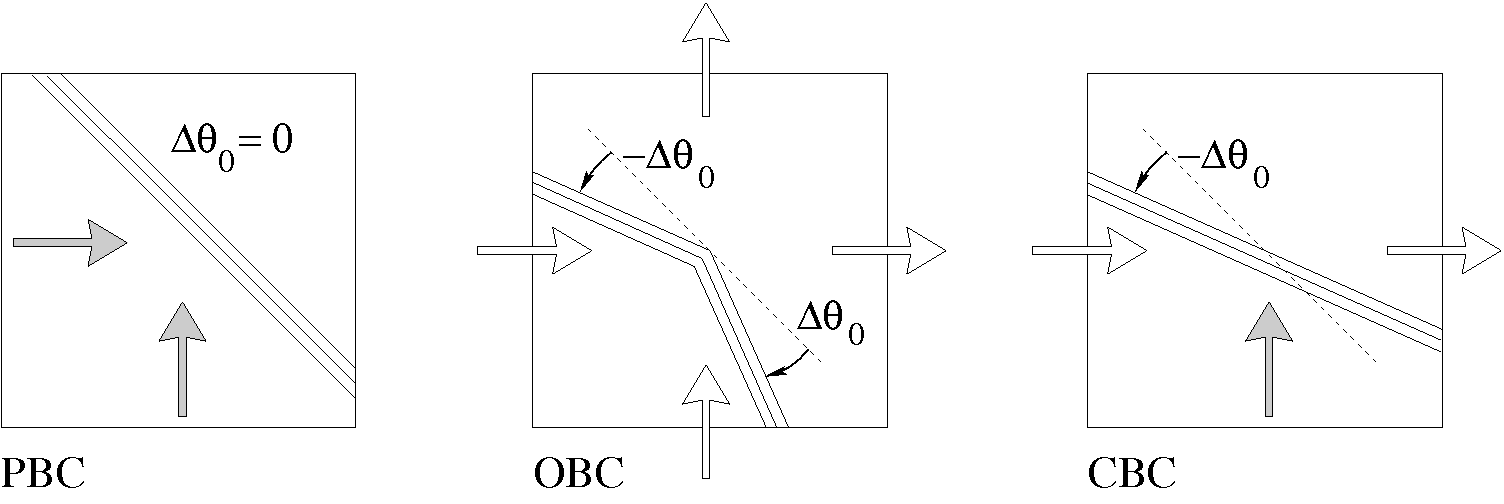
Figure 1: Schematic representation of the intersection square of two perpendicular traffic flows for three different types of boundary conditions: periodic (PBC), open (OBC), and cylindrical (CBC). White arrows correspond to incoming and outgoing fluxes, grey arrows to fluxes that circulate with periodic boundaries. The dashed lines are for reference and are at $45^{\circ}$ with respect to the main axes. Solid lines indicate the average orientation of the striped pattern; the angle differences $\pm\Delta\theta_{0}$ with respect to the line of reference have been exaggerated for greater clarity. For OBC the pattern is chevron-like, for CBC only one branch of the chevron persists.

This paper is organized as follows. In section 2 we describe the particle model. In section 3 we relate it to a corresponding mean-field model. In section 4 we simulate the particle system with PBC. We exhibit the instability by which a uniform initial state develops into a stationary state with a diagonal pattern of stripes. We explain this phenomenon in terms of a linear stability analysis of the mean field model. In section 5 we simulate the same stripe formation instability with OBC. We point out the chevron effect which, whereas absent for PBC, appears under OBC both in the particle and the mean field model. We discuss two methods of measuring and quantifying the chevron angle $\Delta\theta_{0}$, the ‘crest method’ and the ‘velocity ratio method’, and show by simulation that $\Delta\theta_{0}$ is linear in the particle density. In section 6 we provide an elementary theoretical argument that explains the chevron effect. In section 7 we simulate the mean field model with CBC. In this case there is a control parameter for each of the two directions (basically the densities of the two particle fluxes), and we determine how $\Delta\theta_{0}$ depends on them. Whereas all the above work deals with stationary states, in section 7.2 we shed additional light on the chevron effect by studying it in a transient. In section 8 we present a summary of our results and conclude.

2 Particle model

2.1 Geometry

A ‘street of width $M$’ is modeled on a lattice as a set of $M$ parallel infinite one-dimensional lanes. Two such streets intersecting at a right angle lead to the geometry of Fig. 2. The heavy line surrounds the $M\times M$ intersection square, whose sites we will denote by $\mathbf{r}=(i,j)$ with $1\leq i,j\leq M$. At a large distance $L$ from the intersection square, eastbound $({\rm E})$ and northbound $({\rm N})$ particles are injected onto the ‘injection sites’ (the ones indicated by arrows in Fig. 2) of the the horizontal and vertical lanes, respectively, with a probability $\alpha$ per unit time interval for each empty injection site. Each particle stays in its lane and advances by steps of a single lattice unit according to an update scheme to be discussed below. The $(1,1)$ diagonal through the origin is, statistically, an axis of symmetry. The geometry described here was introduced and studied in Ref. [20]; there, however, the focus was on the jamming transitions that occur when $\alpha$ exceeds a critical value $\alpha_{\rm c}(M)$, which for the $M$ values considered in this work is typically of the order of $0.10$ . In the present study we will consider the model in the regime of low $\alpha$. We will employ two distinct update schemes.

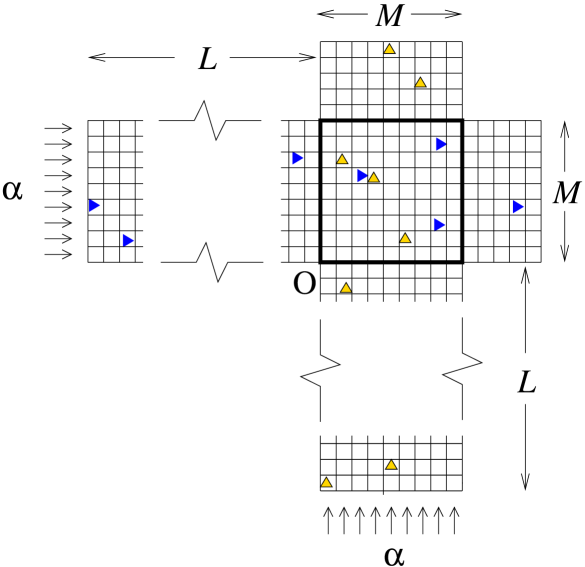
Figure 2: The intersection of two streets of width $M$ is the $M\times M$ square lattice surrounded in bold. Eastbound particles are represented by blue triangles pointing right and northbound ones by orange ones pointing upward. The symbol ‘O’ denotes the origin of the coordinate system; the site in the lower left corner of the square has coordinates $(1,1)$. The influx of particles takes place at a large distance $L$ from the intersection square and is controlled by a parameter $\alpha$.

2.2 Update schemes

The first update scheme that we will use is the frozen shuffle update [22, 23, 11]. Under this scheme, each particle $\ell$ that enters the system is assigned a phase $\tau_{\ell}\in[0,1)$ [23], which it keeps until it leaves the system again; its position is then updated at the instants $t+\tau_{\ell}$ on the continuous time axis, where $t$ is an integer. An update consists in moving the particle one site ahead unless its target site is occupied. Hence during a unit interval all particles positions are updated once, and this happens in order of increasing phases (the ‘update sequence’).

This update is suitable for pedestrians because it reproduces step cycles with a distribution of phases.

The second update scheme that we will use is the alternating parallel update, in which the ${\rm E}$ particles are updated in parallel at half-integer times and the ${\rm N}$ particles all in parallel at integer times. An update consists in simultaneously moving all those particles whose target site is empty.

In two-dimensional situations such as occur on the intersection square, both schemes have the advantage of avoiding ‘conflicts’, that is, of providing a natural priority rule when two perpendicularly traveling particles target the same site. At the relatively low particle densities that we are concerned with here, our simulations will show that many features of the behaviour of the system are qualitatively the same for both update schemes.

2.3 Open-ended boundary conditions

In the street sections of length $L$ waiting lines may form at the entrance of the intersection square. For $\alpha<\alpha_{\rm c}(M)$ this waiting line has a fluctuating length of some finite stationary average value and we will say that the system is in the free flow phase. The opposite case, $\alpha>\alpha_{\rm c}(M)$, leads to a jammed phase and will not concern us here. In the free flow phase the control parameter $\alpha$ entirely determines the average injected current $J(\alpha)$, which is also equal to the current passing through each lane. The expressions are

$$J(\alpha)=\left\{\begin{array}[]{ll}\alpha/(1+\alpha),&\mbox{alternating parallel update},\\[5.69054pt] a/(1+a),&\mbox{frozen shuffle update}.\end{array}\right.$$ (1)

in which $a\equiv-\log(1-\alpha)$ is the injection rate  corresponding to $\alpha$. The first one of relations (1) is well-known and the second one was derived in Ref. [23]. Both lead to $J(\alpha)\simeq\alpha$ in the small $\alpha$ (low density) limit.

In practice we chose $L$ (see Fig. 2) larger than the lengths of any waiting lines observed in the simulations, so that effectively $L=\infty$. We therefore have a two-parameter model whose properties depend only on $\alpha$ and $M$.

2.4 Equations for the particle model

For both update schemes the system evolves like a deterministic cellular automaton with stochastic boundary conditions. Let $n^{{\rm E}}_{s}(\mathbf{r})=1$ (or $=0$) if at time $s$ site $\mathbf{r}=(i,j)$ is (or is not) occupied by an eastbound particle. A similar definition holds for $n^{{\rm N}}_{s}(\mathbf{r})$. The update scheme (with $s$ continuous or discrete, as the case may be) and the boundary conditions together determine the time evolution of these occupation numbers. For the case of alternating parallel update the occupation numbers of the eastbound particles satisfy

$$n^{{\rm E}}_{t+\frac{1}{2}}(\mathbf{r})=[1-n^{{\rm E}}_{t-\frac{1}{2}}(\mathbf{r})-n^{{\rm N}}_{t}(\mathbf{r})]n^{{\rm E}}_{t-\frac{1}{2}}(\mathbf{r}-\mathbf{e}_{x})+[n^{{\rm E}}_{t-\frac{1}{2}}(\mathbf{r}+\mathbf{e}_{x})+n^{{\rm N}}_{t}(\mathbf{r}+\mathbf{e}_{x})]n^{{\rm E}}_{t-\frac{1}{2}}(\mathbf{r}),$$ (2)

for any integer $t$ and where $\mathbf{e}_{x}$ is the unit vector along the $i$ direction; and those for the northbound particles satisfy an analogous equation relating their values at the integer times $t+1$ to those at $t$. For frozen shuffle update described in section 2.2, in contrast to the simplicity of the numerical algorithm, the analytic expression for the time evolution equations is quite cumbersome and we will not display it.

Of interest are, for each update scheme, the mean values $\langle n^{{\rm E},{\rm N}}_{t}(\mathbf{r})\rangle$, where the average $\langle\ldots\rangle$ is over the stochastic boundary conditions at the injection sites and possibly over stochastic initial conditions at time $t=0$.

3 Mean field model

3.1 Equations for the mean field model

In this section we will juxtapose the particle model formulated in terms of the binary variables $n^{{\rm E}}_{t}(\mathbf{r})$ and $n^{{\rm N}}_{t}(\mathbf{r})$ with a mean field description in terms of continuous fields $\rho^{{\rm E}}_{t}(\mathbf{r})$ and $\rho^{{\rm N}}_{t}(\mathbf{r})$, the latter being thought of as representing local averages. With the purpose of retaining only the strict minimum of terms we introduce one further approximation, that consists in neglecting in (2) the interactions between particles of the same kind. A partial justification for this runs as follows. Let $\rho$ be the typical density of each of the two particle types in the intersection square. In the low density limit the positions of the E particles are not correlated with those of the N particles, and hence the frequency of a local blocking event between two particles of different types tends to zero as the square of their density, $\sim\rho^{2}$. On the contrary, two consecutive same-type particles in the same lane (a ‘leader’ and a ‘follower’, say of type E) have their positions and speeds correlated in such a way that the leader cannot block the follower unless it is first blocked itself by an N particle; and the frequency of such a local three particle event is proportional to $\rho^{3}$.

When we average equations (2), correlations between occupation numbers appear. We obtain a closed system of equations through the mean field approximation that consists in factorizing these correlations, that is, we simply repace in (2) the $n^{{\rm E},{\rm N}}_{t}(\mathbf{r})$ by their averages $\rho^{{\rm E},{\rm N}}_{t}(\mathbf{r})$. If moreover we pass from alternating parallel to fully parallel update, we get

$$\rho^{{\rm E}}_{t+1}(\mathbf{r})=[1-\rho^{{\rm N}}_{t}(\mathbf{r})]\rho^{{\rm E}}_{t}(\mathbf{r}-\mathbf{e}_{x})+\rho^{{\rm N}}_{t}(\mathbf{r}+\mathbf{e}_{x})\rho^{{\rm E}}_{t}(\mathbf{r}),$$ (3)

$$\rho^{{\rm N}}_{t+1}(\mathbf{r})=[1-\rho^{{\rm E}}_{t}(\mathbf{r})]\rho^{{\rm N}}_{t}(\mathbf{r}-\mathbf{e}_{y})+\rho^{{\rm E}}_{t}(\mathbf{r}+\mathbf{e}_{y})\rho^{{\rm N}}_{t}(\mathbf{r}).$$

These equations define what we will refer to as the mean field model. It is hard to assess a priori  the quality of the approximation involved in going from the particle model to (3), whatever the update be. In the following sections we will solve Eqs. (3) numerically under a variety of boundary conditions and observe that the behavior of the densities $\rho^{{\rm E},{\rm N}}_{t}(\mathbf{r})$ is qualitatively close to that of the particle densities in the particle model. We will then take this correspondence as an a posteriori  confirmation that Eqs. (3) make sense.

Linearized equations.   We notice that a uniform density distribution $\rho^{{\rm E},{\rm N}}_{t}(\mathbf{r})=\overline{\rho}$  solves Eqs. (3). Setting $\rho^{{\rm E},{\rm N}}_{t}(\mathbf{r})=\overline{\rho}+\delta\rho^{{\rm E},{\rm N}}_{t}(\mathbf{r})$ and linearizing these equations in $\delta\rho^{{\rm E},{\rm N}}_{t}$ one obtains

$$\delta\rho^{{\rm E}}_{t+1}(\mathbf{r}) =(1-\overline{\rho})\delta\rho^{{\rm E}}_{t}(\mathbf{r}-\mathbf{e}_{x})-\overline{\rho}\delta\rho^{{\rm N}}_{t}(\mathbf{r})+\overline{\rho}\delta\rho^{{\rm E}}_{t}(\mathbf{r})+\overline{\rho}\delta\rho^{{\rm N}}_{t}(\mathbf{r}+\mathbf{e}_{x}),$$

$$\delta\rho^{{\rm N}}_{t+1}(\mathbf{r}) =(1-\overline{\rho})\delta\rho^{{\rm N}}_{t}(\mathbf{r}-\mathbf{e}_{y})-\overline{\rho}\delta\rho^{{\rm E}}_{t}(\mathbf{r})+\overline{\rho}\delta\rho^{{\rm N}}_{t}(\mathbf{r})+\overline{\rho}\delta\rho^{{\rm E}}_{t}(\mathbf{r}+\mathbf{e}_{y}).$$

In this study we will, on the one hand, perform simulations of the particle model, and on the other hand investigate the numerical solution of the mean field model (3). We will briefly mention some analytic work that may be done on (LABEL:mfeqns2dlin).

3.2 Open-ended boundary conditions

For the mean-field equations (3) we implement the open-ended boundary conditions (OBC) for simplicity in a way slightly different from how we applied them to the particle system. We will in fact restrict the simulation to the intersection square, that is, to the lattice sites $\mathbf{r}=(i,j)$ with $1\leq i,j\leq M$. Equations (3) couple the boundary site $\mathbf{r}=(1,j)$ to the site $\mathbf{r}-\mathbf{e}_{x}=(0,j)$ outside this square. We will refer to the sites $(0,j)$ and $(i,0)$ as the entrance sites at the west and south boundary, respectively, of the intersection square. Instead of imposing the injection rate $\alpha$ a large distance $L$ away from the intersection square, as we did for the particle model, we will suppress the street segments of length $L$ leading up to the square and impose at each instant of time $t$ the random entrance site densities

$$\rho^{{\rm E}}_{t}(0,k)=\eta^{{\rm E}}_{t}(k),\qquad\rho^{{\rm N}}_{t}(k,0)=\eta^{{\rm N}}_{t}(k),$$ (5)

for all $k=1,2,\ldots,M$, where the $\eta^{{\rm E},{\rm N}}_{t}(k)$ are i.i.d. random variables $\eta$ of average $\overline{\eta}$. In actual practice, supposing that the details of their probability law are unimportant, we drew them from the uniform distribution

$$p(\eta;\overline{\eta})=\left\{\begin{array}[]{ll}{1}/{\overline{\eta}},&\frac{1}{2}\overline{\eta}<\eta<\frac{3}{2}\overline{\eta},\\[5.69054pt] 0,&\mbox{else}.\end{array}\right.$$ (6)

With the random boundary conditions (5) the $\rho^{{\rm E},{\rm N}}_{t}(\mathbf{r})$ become random variables and we will indicate their averages by $\langle\rho^{{\rm E},{\rm N}}_{t}(\mathbf{r})\rangle$.

As exit boundary conditions we take $\rho^{{\rm E}}_{t}(M+1,k)=\rho^{{\rm N}}_{t}(k,M+1)=0$, which expresses that the particles freely leave the system. Note that when complemented with these exit boundary conditions, Eqs.(3) are not solved anymore by a uniform density for a finite system but lead to a boundary effect at the exit. Thus Eqs.(LABEL:mfeqns2dlin) can rigorously be regarded as the linearization of Eqs.(3) only in the $M\rightarrow\infty$ limit.

With these free exit conditions, the currents through each of the $2M$ lanes are determined by the entrance boundary conditions. As these are expressed in Eq.(5) as density boundary conditions, we must expect the currents $J_{k}(\overline{\eta})$ to depend on the lane index $k$; this dependency, however, has turned out to be extremely weak in all situations studied in this work.

Finally, whereas the mean field model of basic interest has the open boundary conditions described above, we will also be led, in the sections below to replace these with periodic boundary conditions in one or both of the directions.

4 Crossing flows on a torus

In order to understand the basic mechanism of the stripe formation we first study, in this section, a simplified problem in which the interaction square is submitted to periodic boundary conditions (PBC) in both directions. This procedure was first proposed by Biham et al. [12] and later followed by several other authors [13]. The results from such a study on a torus are thus of interest in their own right. Our investigation includes an analytic calculation which explains the instability observed on the torus in our own and in earlier simulations. Moreover, our PBC results will serve as a basis for comparison when in the next section we study the original problem, that is, the intersection square with open boundaries (OBC).

4.1 Stripe formation in the particle model

We consider a particle system with frozen shuffle update and impose on the intersection square PBC in both directions of space. At the initial time $2N$ particles ($N$ going east and $N$ going north) are placed on random lattice positions subject to hard core exclusion. For these boundary conditions the space averaged particle density $\overline{\rho}=N/M^{2}$ replaces $\alpha$ as the control parameter. Choosing the phases $\{\tau_{\ell}\}$ of a conserved set of particles amounts to choosing a fixed random permutation of them. They are then updated at each time step in that order. The system therefore is a deterministic cellular automaton: its initial state determines, via  the update scheme, its entire time evolution.

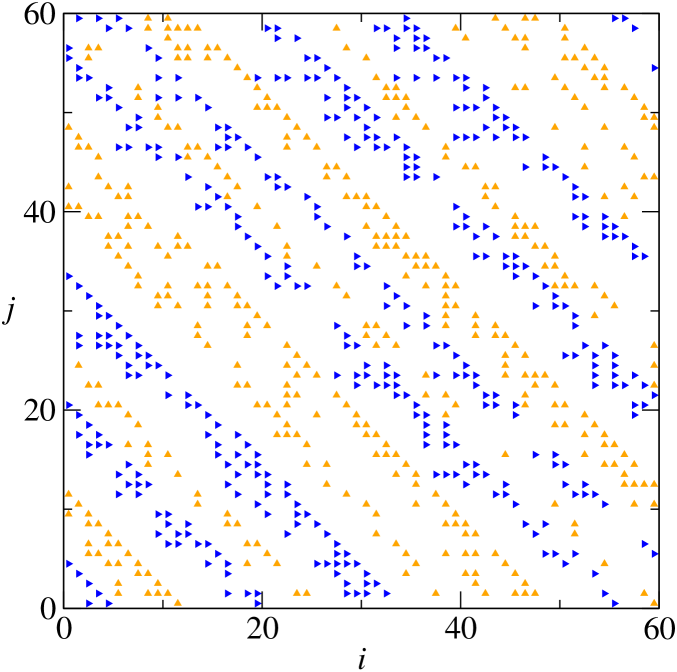
Figure 3: Snapshot of the stationary state of a particle simulation with frozen shuffle update and periodic boundary conditions, for system size $M=60$ and particle density $\overline{\rho}=0.1$. Particles of the same type are aligned along diagonals in the $(1,-1)$ direction that have a width of a few lattice distances. The simulation was carried out by Chloé Barré, who also prepared this figure.

Simulations show that after a certain transient time $t_{\rm trans}$ the uniform particle distribution becomes unstable. Fig. 3 shows what happens for the example of a street width $M=60$ containing 720 particles: the system self-organizes into a pattern of alternating diagonals of same-type particles that are at an angle of $45^{\circ}$. The wavelength of the pattern is typically in the range from 5 to 15 lattice distances; it is irregular, its details depending on the initial condition. The system eventually enters a limit cycle in which all or almost all particles move at each time step.

In the limit of small $\overline{\rho}$ limit we found that roughly $t_{\rm trans}\sim 1/\overline{\rho}$. For the linear lattice size $M=60$ (measured in lattice units) and the low particle densities $0.02\lesssim\overline{\rho}\lesssim 0.10$ that we considered, we found that $t_{\rm trans}$ (measured in time steps) may be up to an order of magnitude larger than the lattice size $M$. This sets a limit to what we can learn from this PBC study about the behavior of the open system: if $t_{\rm trans}\gtrsim M$, the particles entering the open intersection square will not be able to fully develop their instability before they quit the system again. We will return to this point in section 5.

4.2 Stripe formation instability of the mean field model

Linear regime.   In order to explain the origin of the instability analytically, we will now perform a stability analysis on the linearized mean field equations (LABEL:mfeqns2dlin) with PBC. Let us define the Fourier transforms

$$\hat{\rho}^{{\rm E},{\rm N}}_{t}(\mathbf{q})=\sum_{k=1}^{M}\sum_{l=1}^{M}{\rm e}^{{\rm i}\mathbf{q}\cdot\mathbf{r}}\,\delta\rho^{{\rm E},{\rm N}}_{t}(k,l)$$ (7)

where $\mathbf{q}=(q_{x},q_{y})$ with $q_{x,y}=2\pi\kappa_{x,y}/{M}$ and $\kappa_{x,y}=0,1,\ldots,M-1$. The linearized equations then read

$$\left(\begin{array}[]{r}\delta\hat{\rho}^{{\rm E}}_{t+1}(\mathbf{q})\\ \delta\hat{\rho}^{{\rm N}}_{t+1}(\mathbf{q})\end{array}\right)=\left(\begin{array}[]{cc}{\rm e}^{{\rm i}q_{x}}R_{q_{x}}&R_{q_{x}}-1\\ R_{q_{y}}-1&{\rm e}^{{\rm i}q_{y}}R_{q_{y}}\end{array}\right)\left(\begin{array}[]{r}\delta\hat{\rho}^{{\rm E}}_{t}(\mathbf{q})\\ \delta\hat{\rho}^{{\rm N}}_{t}(\mathbf{q})\end{array}\right),$$ (8)

where $R_{q}=1+\overline{\rho}({\rm e}^{-{\rm i}q}-1)$. One of the eigenvalues of the $2\times 2$ matrix in (8) is always inside the unit circle. The other one, which we will call $\mu_{0}(\mathbf{q})$, is given by

$$\mu_{0}(\mathbf{q})=\frac{1}{2}\Big{(}{\rm e}^{{\rm i}q_{x}}R_{q_{x}}+{\rm e}^{{\rm i}q_{y}}R_{q_{y}}+\big{[}({\rm e}^{{\rm i}q_{x}}R_{q_{x}}-{\rm e}^{{\rm i}q_{y}}R_{q_{y}})^{2}-4(R_{q_{x}}-1)(R_{q_{y}}-1)\big{]}^{1/2}\Big{)}.$$ (9)

We found numerically that its absolute value $|\mu_{0}(\mathbf{q})|$ has a maximum on the diagonal $q_{x}=q_{y}$, as shown in Fig. 4. This maximum exceeds unity and is therefore associated with an unstable mode traveling in the $(1,1)$ direction with wavelength

$$\lambda_{\rm max}=2\pi/|\mathbf{q}|_{\rm max} = \sqrt{2}\pi/\arccos[(1-2\overline{\rho})/(2-2\overline{\rho})]$$ (10)

$$= 3\sqrt{2}[1-(\sqrt{3}/\pi)\overline{\rho}]+{\cal O}(\overline{\rho}^{2}),$$

where in the second line we expanded for small $\overline{\rho}$. This calculation thus explains the formation of a diagonal striped pattern as a consequence of the unstable Fourier modes present in a random initial state.

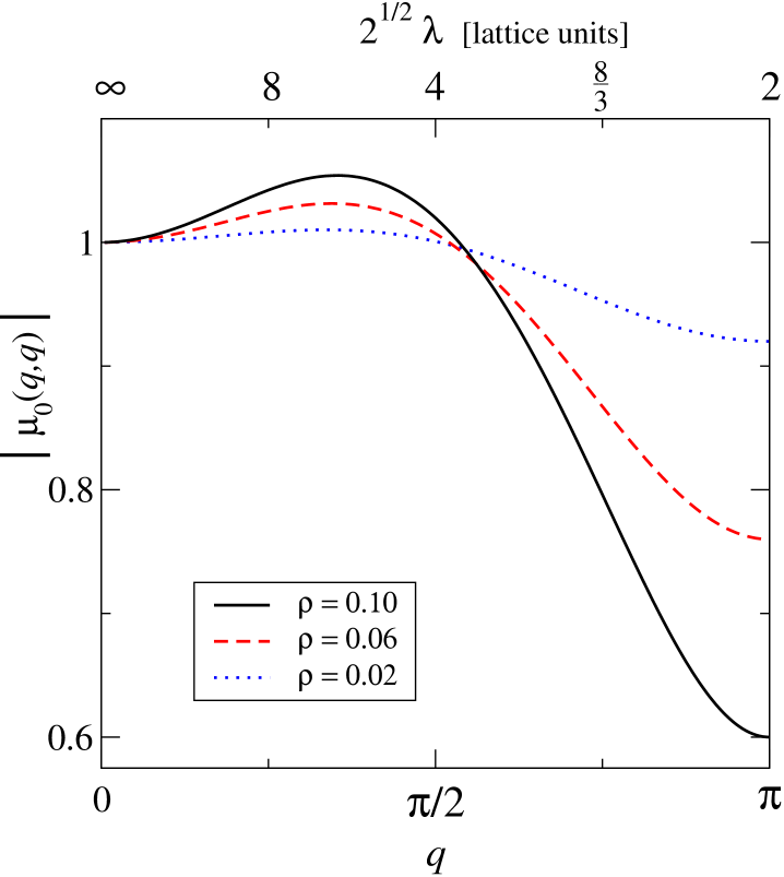
Figure 4: Larger absolute eigenvalue $|\mu_{0}(\mathbf{q})|$ along the diagonal as a function of the wavenumber $q=q_{x}=q_{y}$. The upper axis shows the corresponding wavelength $\lambda=2\pi/q$.

Nonlinear regime.   The nonlinear regime of the mean field equations, Eqs. (3), is outside the reach of this analysis. Numerical solution of (3) with PBC shows that the solution tends to a stationary state consisting of alternating stripes having on each site $\mathbf{r}$ either $\rho^{{\rm E}}_{t}(\mathbf{r})\neq 0$ or $\rho^{{\rm N}}_{t}(\mathbf{r})\neq 0$; and in which consecutive stripes are separated by unoccupied sites in such a way that all nonlinear terms in (3) vanish. The density patterns $\rho^{{\rm E}}_{t}(\mathbf{r})$ and $\rho^{{\rm N}}_{t}(\mathbf{r})$ then advance at unit speed unimpeded eastward and northward, respectively, around the torus, in a way perfectly similar to the particles in section 4.1. In the final state under PBC, therefore, the coupling between the two particle types has disappeared.

Armed with this understanding we now return to the original problem of the open intersection square.

5 Open intersection

We now address the central question of this work, that is, how do two flows cross on an open square? The control parameters are those defined in sections 2 and 3, namely the injection probability $\alpha$ in the case of the particle model, and the boundary density $\overline{\eta}$ at the entrance sites in the case of the mean field model. Whereas under PBC the final stationary state was determined by the randomly selected initial state, under OBC it is a consequence of the noise coming from the entrance boundaries. In all the simulations and numerical calculations below we took statistics only after a transient time sufficiently long for the system to settle in a stationary state. Typically, this time was of the order of a few times the linear lattice size $M$.

5.1 Stripe formation in the particle model

In simulations restricted to linear sizes $M$ less than, say, a few tens of lattice distances, the particles seem to fill the intersection square largely randomly. However, as $M$ grows, one may discern more or less clear cut local alignments of same-type particles along diagonals, as shown in the snapshot in Fig. 5, where $M=60$ and $\alpha=0.09$. We therefore investigated what happens for much larger $M$. It then appears that, far enough from the boundaries, the particles form alternating stripes in the same way as observed for PBC. This is exemplified in Fig. 6, where $M=640$ and $\alpha=0.09$.

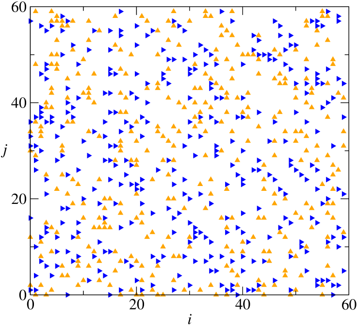
Figure 5: Snapshot of the stationary state of the intersection square in a particle simulation with open boundary conditions, for $\alpha=0.09$ and $M=60$. The blue particles ( $\blacktriangleright$) come from the left and the orange ones ( $\blacktriangle$) from the bottom. Obtained with frozen shuffle update.

Furthermore the following observations are of interest. Along the two entrance boundaries an $\alpha$ dependent penetration depth  $\xi(\alpha)$ characterizes the distance that a randomly entering group of particles needs to travel before it gets to self-organize into stripes. For $\alpha=0.09$ the figure shows that $\xi(\alpha)\approx 50$; for $\alpha\to 0$ we found that this penetration depth diverges roughly as $\xi(\alpha)\sim\alpha^{-1}$. The organization into stripes reduces the probability of ${\rm E}/{\rm N}$ and ${\rm N}/{\rm E}$ blockings to below their values for a random distribution of particles, and it therefore increases the particles’ average velocity. Finally, we observe that the stripes are well-separated from one another and move almost without any mutual penetration. This is borne out more clearly by the zoom shown in Fig. 7, to which we will return later.

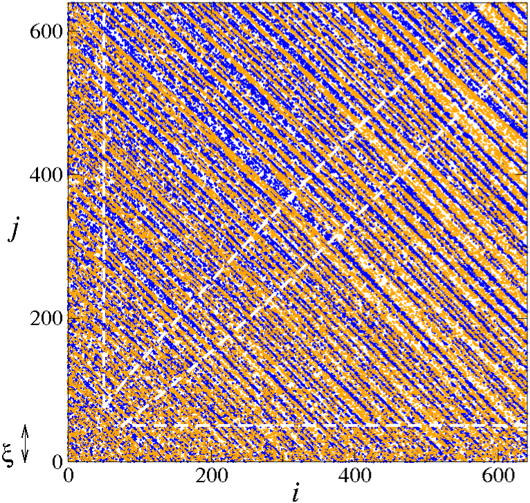
Figure 6: Snapshot of the stationary state of the intersection square of a particle system with $M=640$ and $\alpha=0.09$ and subject to frozen shuffle update. The blue particles are eastbound the orange ones northbound. Between the lower-left and the upper-right the particles self-organize to form a diagonal pattern. The white dashed lines delimit the transition zone between the upper and lower triangular regions as discussed in section 5.3. Along the two entrance boundaries there are disordered boundary layers of width $\xi\approx 50$.

5.2 Stripe formation in the mean field model

Nonlinear equations.   We have numerically solved the nonlinear mean field equations (3) on the intersection square, imposing time dependent random densities as described in section 3.2 on the entrance sites along the west and south boundaries, and free exit conditions along the other two boundaries. The system rapidly relaxes to a stationary state independent of the initial condition at time $t=0$; in our numerical resolution we took for the latter $\rho^{{\rm E}}_{0}(\mathbf{r})=\rho^{{\rm N}}_{0}(\mathbf{r})=\overline{\rho}_{0}$ for all $\mathbf{r}=(i,j)$ with $1\leq i,j\leq M$.

The stripe structure becomes visible when we color a site blue or orange according to whether $\rho^{{\rm E}}(\mathbf{r})$ is larger or smaller than $\rho^{{\rm N}}(\mathbf{r})$. The result at time $t=1000$ is shown in Fig. 8. Hence the mean field equations with OBC lead to the same stripe formation as they did with PBC. There is, similarly, a penetration depth along the entrance boundaries within which the stripe structure has not yet developed. The depth is here dependent on the average imposed boundary density $\overline{\eta}$.

Linearized equations.   The Green function of the linearized equations (LABEL:mfeqns2dlin) represents the response of the system to an isolated boundary field $\eta^{{\rm E},{\rm N}}(\mathbf{r},t)$ acting at time $t=t_{0}$ on a single entrance site $\mathbf{r}=(0,j)$ or $\mathbf{r}=(i,0)$. This Green function is easily computed numerically, but may also be determined analytically. The analytical calculation leads to an expression for several quantities of interest, among which the wavelength of the pattern of stripes,

$$\lambda=\sqrt{2}\pi/\arctan[(3-4\overline{\eta})^{1/2}/(1-2\overline{\eta})]\,.$$ (11)

The calculation is very lengthy and will be presented elsewhere [24].

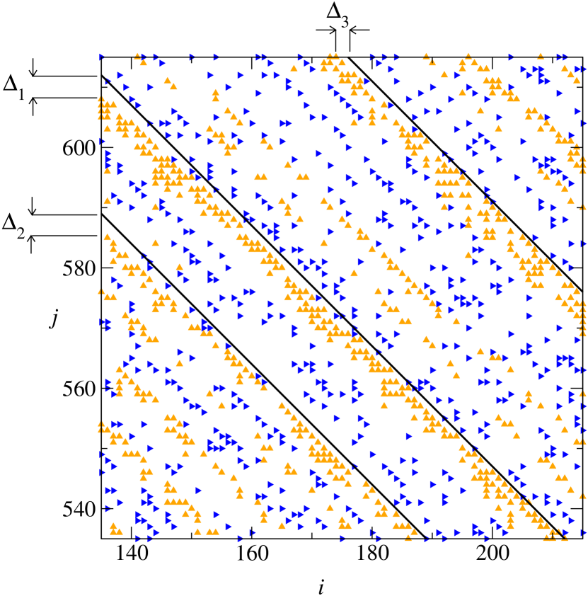
Figure 7: Zoom on a region of Fig. 6 showing the chevron pattern. This snapshot has been taken for $M=640$ and $\alpha=0.09$. The black solid lines are at an angle of $45^{\circ}$. The nonzero distances $\Delta_{1},\Delta_{2},$ and $\Delta_{3}$ show that there is a negative $\Delta\theta$. Moreover, the northbound particles appear to be confined, statistically, to narrower strips than the eastbound ones.

A remark.   A comment is needed about the stability of Eqs. (3). The solution of these equations, after being perfectly reasonable, may develop a local instability beginning by one of the densities $\rho^{{\rm E}}_{t}$ or $\rho^{{\rm N}}_{t}$ becoming negative at a particular site $\mathbf{r}$, after which in a few time steps the solution tends to infinity in that region. For densities around $0.100$, which are among the highest that we consider here, and for $M=500$, this typically happens after 5000 to 15 000 time steps. For lower densities it is rarer. The average $\langle\ldots\rangle$ at time $t$ is therefore defined as restricted to all histories for which no instability has occurred up to that time. The instability is suppressed if we add higher order nonlinear terms to Eqs. (3), e.g. by replacing $\rho^{{\rm E}}_{t}$ with $1-{\rm e}^{-\rho^{{\rm E}}_{t}}$ in the first of Eqs.(3) and similarly $\rho^{{\rm N}}_{t}$ with $1-{\rm e}^{-\rho^{{\rm N}}_{t}}$ in the second one. In that case one easily shows that for initially positive densities and appropriate boundary conditions the solution must stay positive at all times. Simulations with this exponential density dependence give results very close to the ones obtained from Eqs. (3).

5.3 Chevron effect

Having found that both the particle and the mean field model are subject to the pattern formation instability, we continue in this subsection our investigation of the pattern structure.

Closer examination of Fig. 6 (particle model with frozen shuffle update) and Fig. 8 (mean field model with density boundary conditions) reveals an effect just barely visible to the eye (it is better visible if the paper is held flat!), namely that the angle $\theta$ of the striped pattern, is not exactly equal to  $45^{\circ}$ but differs systematically from it by an amount $\Delta\theta(\mathbf{r})$ which is of the order of a degree. This angle difference $\Delta\theta(\mathbf{r})$ is negative above the axis of symmetry and positive below it, so that the stripes acquire the character of chevrons, as schematically represented in Fig. 1b; we will therefore call this the ‘chevron effect’ and refer to $\Delta\theta(\mathbf{r})$ as the ‘chevron angle’. We have verified that the chevron effect also occurs in the particle model with alternating parallel update and show proof of this in Fig. 9.

From the fact that it appears under all these different conditions we conclude that it is a robust property of a wide class of intersecting flow models. We note, however, that no sign of the chevron effect appeared in the linear stability analysis mentioned in section 5.1 above; hence the effect is essentially connected to the nonlinearity of the evolution equations.

We will now investigate the quantitative relation between $\theta(\mathbf{r})$ and the control parameters, $\alpha$ or $\overline{\eta}$. A prerequisite is that we define this angle in a way allowing us to quantify it operationally in the simulations. We will successively discuss two different algorithms that we conceived for this purpose, and that we termed the crest method  and the velocity ratio  method.

5.3.1 Crest method

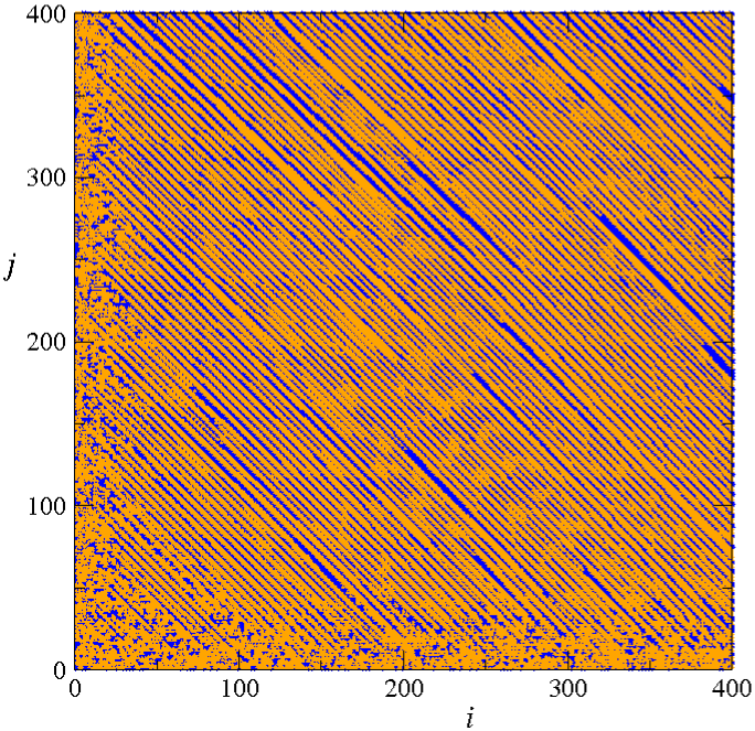
Figure 8: Snapshot representing a typical stationary state configuration of the density fields in an intersection square of size $M=400$ with OBC, subject to a fluctuating boundary density of average $\overline{\eta}=0.06$. A site $\mathbf{r}$ is colored blue or orange according to whether $\rho^{{\rm E}}(\mathbf{r})$ is larger or smaller than $\rho^{{\rm N}}(\mathbf{r})$.

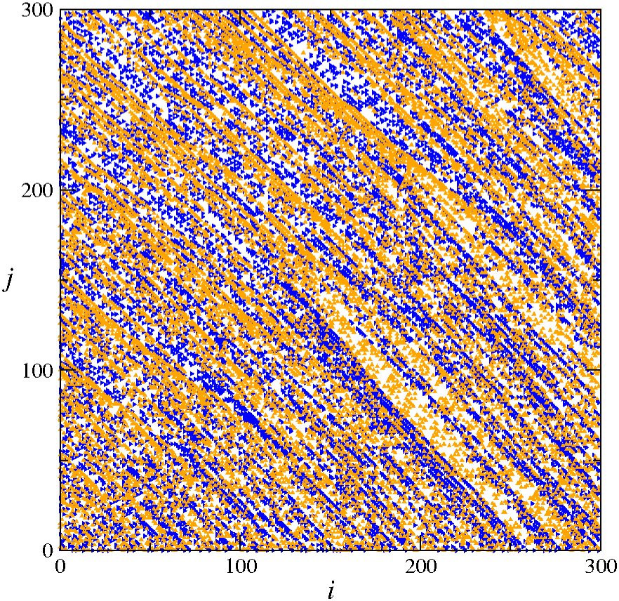
Figure 9: Snapshot of the stationary state of the intersection square of a particle system with $M=300$ and $\alpha=0.15$ and subject to alternating parallel update. The color code is the same as in Fig. 6. The disordered boundary layers along the entrance boundaries are much narrower here than in Fig. 6.

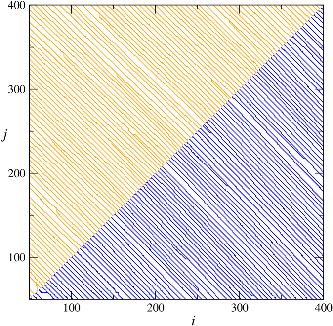
Figure 10: Result of the crest construction algorithm described in section 5.3.1, applied to the density field of Fig. 8. For the value $\overline{\eta}=0.06$ that was used here, the slope of the blue crests (lower triangle) and the orange crests (upper triangle) differs by about $2\Delta\theta_{0}=2.4^{\circ}$. Layers of width 50 along both entrance boundaries were left out of the construction algorithm.

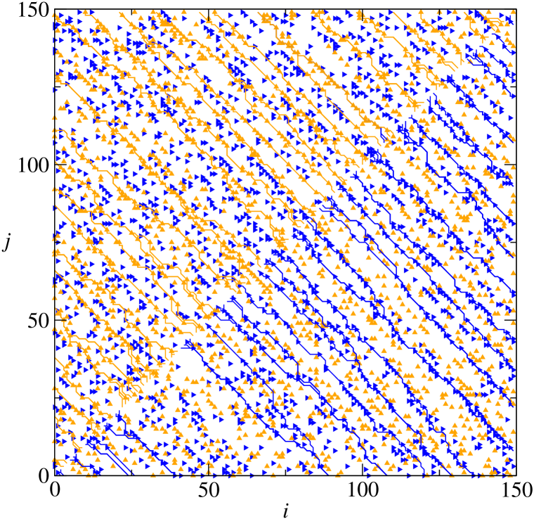
Figure 11: Snapshot of the intersection square for a particle system with $\alpha=0.09$ and $M=150$, obtained with frozen shuffle update. Superimposed are the crests constructed by means of the algorithm of section 5.3.1.

In order to assign a numerical value to the slope $\theta$, we developed an algorithm that closely imitates what visual inspection does: given a configuration of the particle occupation numbers, $\{n^{{\rm E}}(\mathbf{r}),n^{{\rm N}}(\mathbf{r})\}$, or of the density fields, $\{\rho^{{\rm E}}(\mathbf{r}),\rho^{{\rm N}}(\mathbf{r})\}$, it follows the clearly visible crests over a certain distance. This algorithm is easiest to apply to the density fields, their variables being continuous. It is in that case composed of the following steps.

Each diagonal site $\mathbf{r}=(k,k)$ occupied by an eastbound particle is taken as the initial site of a crest to be constructed stepwise towards the south-east. If the current crest end is at $(i,j)$, then the next site on the crest will be one of the three sites $(i,j-1)$, $(i+1,j-1)$, or $(i+1,j)$, whichever has the largest value of $\rho^{{\rm E}}$. The construction ends when the crest reaches the south or east boundary of the intersection square; it may also be restricted to a smaller square resulting from the exclusion of the boundary layers. The end-to-end distance of a crest with initial site $(k,k)$ is a vector that we will denote $\mathbf{c}(k)$. Let $\mathbf{C}^{{\rm E}}=\sum_{k}^{{\rm E}}\mathbf{c}(k)$, where the superscript on the summation sign denotes restriction to initial sites occupied by an eastbound particle. Finally, $\theta$ is taken to be the angle of $\mathbf{C}^{{\rm E}}$. It represents an average over the lower  triangular half of the intersection square. The precision may be increased by repeating the measurement and adding the $\mathbf{C}^{{\rm E}}$ obtained from a sequence of configurations.

Symmetrically, starting from the diagonal sites occupied by a northbound particle, a similarly constructed vector $\mathbf{C}^{{\rm N}}$ leads to a value of $\theta$ averaged over the upper  triangular half of the intersection square. Fig. 10 shows the crests constructed this way for the mean field configuration of Fig. 8.

In a particle configuration the local densities $n^{{\rm E},{\rm N}}(\mathbf{r})$ are binary variables equal to 0 or 1. Before applying the crest algorithm to it, we first create the two density fields $\rho^{{\rm E}}$ and $\rho^{{\rm N}}$ such that $\rho^{{\rm E},{\rm N}}(\mathbf{r})=n^{{\rm E},{\rm N}}(\mathbf{r})$. In order to lift any degeneracies we then apply three diffusion steps in each of which, for the two fields separately, each site distributes a fraction $\epsilon$ of its density content equally over its four neighboring sites (in practice we took $\epsilon=0.1$). After that, the above algorithm can be applied. Fig. 11 shows simultaneously a snapshot of a particle system having $M=150$ and $\alpha=0.09$, and the crests constructed from it.

The same algorithm may serve to construct crests locally and to determine, through an ensemble average, the local values $\theta(\mathbf{r})$. Clearly, too, this algorithm, although natural and making sense, is not unique and different but equally reasonable algorithms might well lead to slightly modified values of the angles $\theta(\mathbf{r})$.

5.3.2 Velocity ratio method

The velocity ratio method for determining the angle $\theta(\mathbf{r})$ is based on an elementary theoretical consideration. Let $v^{{\rm E}}(\mathbf{r})$ and $v^{{\rm N}}(\mathbf{r})$ be the average eastward and northward velocities, respectively, on site $\mathbf{r}$ in the stationary state. The velocities refer to particles or to fields, as the case may be. Under the sole hypothesis, borne out rather well both in the simulations of the particle model and in the numerical solution of the mean field model, that the stripes are mutually impenetrable, the existence of such moving stripes is possible only if locally their angle of inclination $\theta(\mathbf{r})$ is related to their average velocities $v^{{\rm E},{\rm N}}(\mathbf{r})$ by

$$\tan\theta(\mathbf{r})=\frac{v^{{\rm N}}(\mathbf{r})}{v^{{\rm E}}(\mathbf{r})}\,.$$ (12)

In the particle model the velocities are defined by

$$v^{{\rm E},{\rm N}}(\mathbf{r})=\frac{J^{{\rm E},{\rm N}}(\mathbf{r})}{\langle n^{{\rm E},{\rm N}}(\mathbf{r})\rangle},$$ (13)

where $J^{{\rm E},{\rm N}}(\mathbf{r})$ is the stationary current of $\pm$ particles on site $\mathbf{r}$. For the mean field model similar equations hold with the $n$’s replaced with $\rho$’s.

Things simplify in the special case where the boundary conditions impose the same stationary state current $J$ in each horizontal and vertical lane, and hence on each site. In that case, combining (12) and (13) yields, in lieu of (12), an expression for the local slope $\theta(\mathbf{r})$ solely in terms of the two local densities,

$$\tan\theta(\mathbf{r})=\frac{\langle n^{{\rm E}}(\mathbf{r})\rangle}{\langle n^{{\rm N}}(\mathbf{r})\rangle}\,.$$ (14)

Setting $\theta=\frac{\pi}{4}+\Delta\theta$ and expanding (14) to linear order in $\Delta\theta(\mathbf{r})$ yields

$$\Delta\theta(\mathbf{r})\simeq\frac{\langle n^{{\rm E}}(\mathbf{r})\rangle-\langle n^{{\rm N}}(\mathbf{r})\rangle}{2\langle n^{{\rm N}}(\mathbf{r})\rangle}\,,$$ (15)

valid only if $J^{{\rm E},{\rm N}}(\mathbf{r})=J$ is uniform. Eqs. (14) and (15) show, in particular, that there can be a nonzero chevron angle $\Delta\theta(\mathbf{r})$ only if the local densities of the two species are different. Our simulations of the particle model with OBC indeed show this density difference.

5.3.3 Comparison

We will take Eq. (12) as the definition of $\theta(\mathbf{r})$. However, it should be remembered that when the impenetrability hypothesis is violated, the quantity $\theta(\mathbf{r})$ defined by (12) loses its interpretation as the slope of a stripe. This happens near the two entrance boundaries: the disorderly structure within a distance $\xi$ from these boundaries renders the slope ill-defined, even though blind application of Eq. (12) gives a precise value.

When well-defined stripes do exist, one expects the crest algorithm and the velocity ratio method to yield, if not identical, then at least closely similar results. For all situations that we have considered this turns out to be the case. A comparison of the two determinations of $\theta(\mathbf{r})$ will be made in section 5.3.5 (see Fig. 14) and in section 7 (see Fig. 19).

5.3.4 Space dependence of $\Delta\theta(\mathbf{r})$

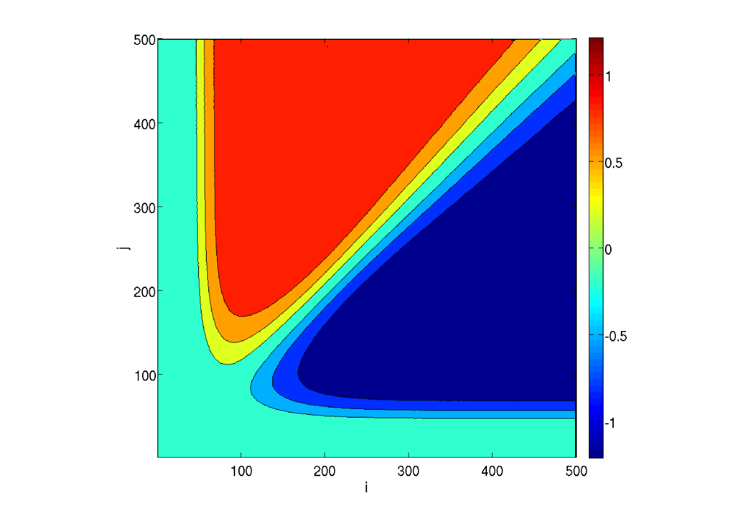
Figure 12: Level plot of the space dependent chevron angle $\Delta\theta(i,j)$ (in degrees), in the stationary state, obtained from the mean field equations (3) by the velocity ratio method, on a square lattice of linear size $M=500$ with open boundary conditions and with $\overline{\eta}^{{\rm E}}=\overline{\eta}^{{\rm N}}=0.06$.

Fig. 12 shows the space dependence of the chevron angle in the intersection square with OBC after the system has attained its stationary state. It has been obtained by the velocity ratio method, Eq. (12), from the solution of the nonlinear mean field equations (3). An average over $10^{5}$ time steps has been performed. This figure provides quantitative support for the observation, already strongly suggested by Fig. 6, that we may divide the intersection square into reasonably well-defined regions according to the value of $\Delta\theta(\mathbf{r})$.

(a) In layers of width $\xi$ along the two entrance boundaries $\Delta\theta(\mathbf{r})$ fluctuates around zero. One of the particle types is here clearly not organized into stripes. As a consequence, the impenetrability hypothesis is violated and the values obtained for $\Delta\theta(\mathbf{r})$ in these boundary layers, although unambiguously defined by (12), do not represent angles of inclination.

(b) There are, clearly visible in Fig. 12, two triangular regions where $\Delta\theta(\mathbf{r})$ is close to constant. We will denote the value of this constant by $\pm\Delta\theta_{0}$ in the lower and upper triangle, respectively.

(c) Along the axis of symmetry there is a transition zone where $\Delta\theta(\mathbf{r})$ passes from $-\Delta\theta_{0}$ above the axis to $+\Delta\theta_{0}$ below it. In Fig. 6 this variation causes a slight rounding at the tips of the chevrons. The transition zone is clearly visible in Fig. 12 and has been indicated by heavy white dashed lines in Fig. 6.

In Fig. 13 we show the analogous plot for a particle model on a square lattice of linear size $M=640$. Regions similar to those in Fig. 6 are visible. For this model we have chosen $\alpha=0.15$, a value just below its jamming point, which gives rise to a chevron angle $\Delta\theta_{0}\approx 4^{\circ}$.

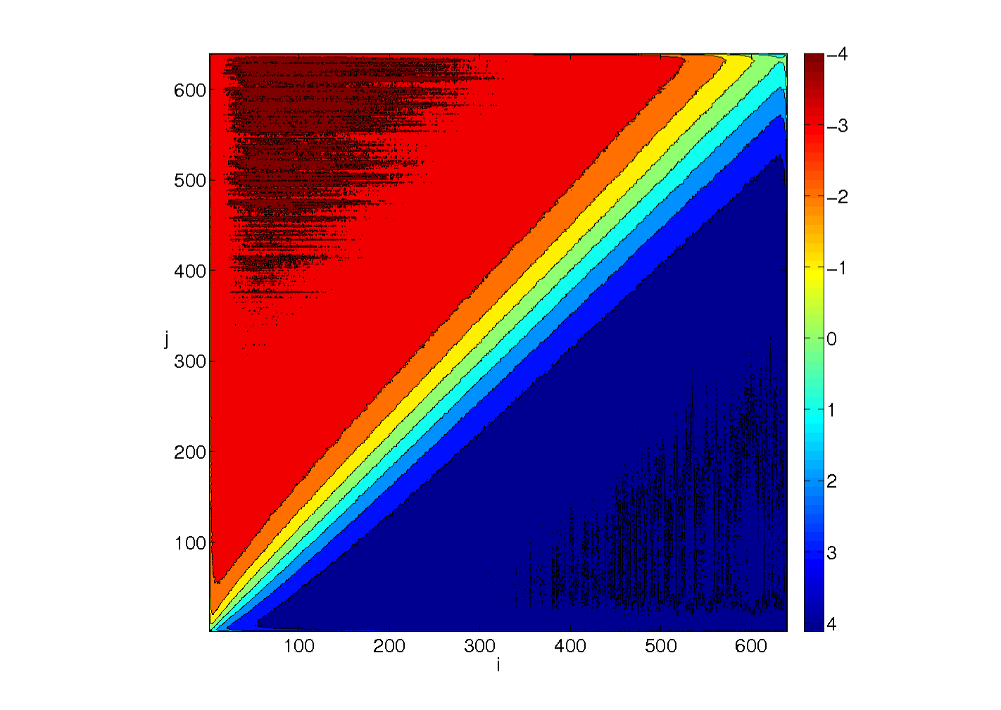
Figure 13: Level plot of the space dependent chevron angle $\Delta\theta(i,j)$ (in degrees), in the stationary state, obtained by the velocity ratio method for a particle model with alternating parallel update on a square lattice of linear size $M=640$ with open boundary conditions and with $\alpha=0.15$.

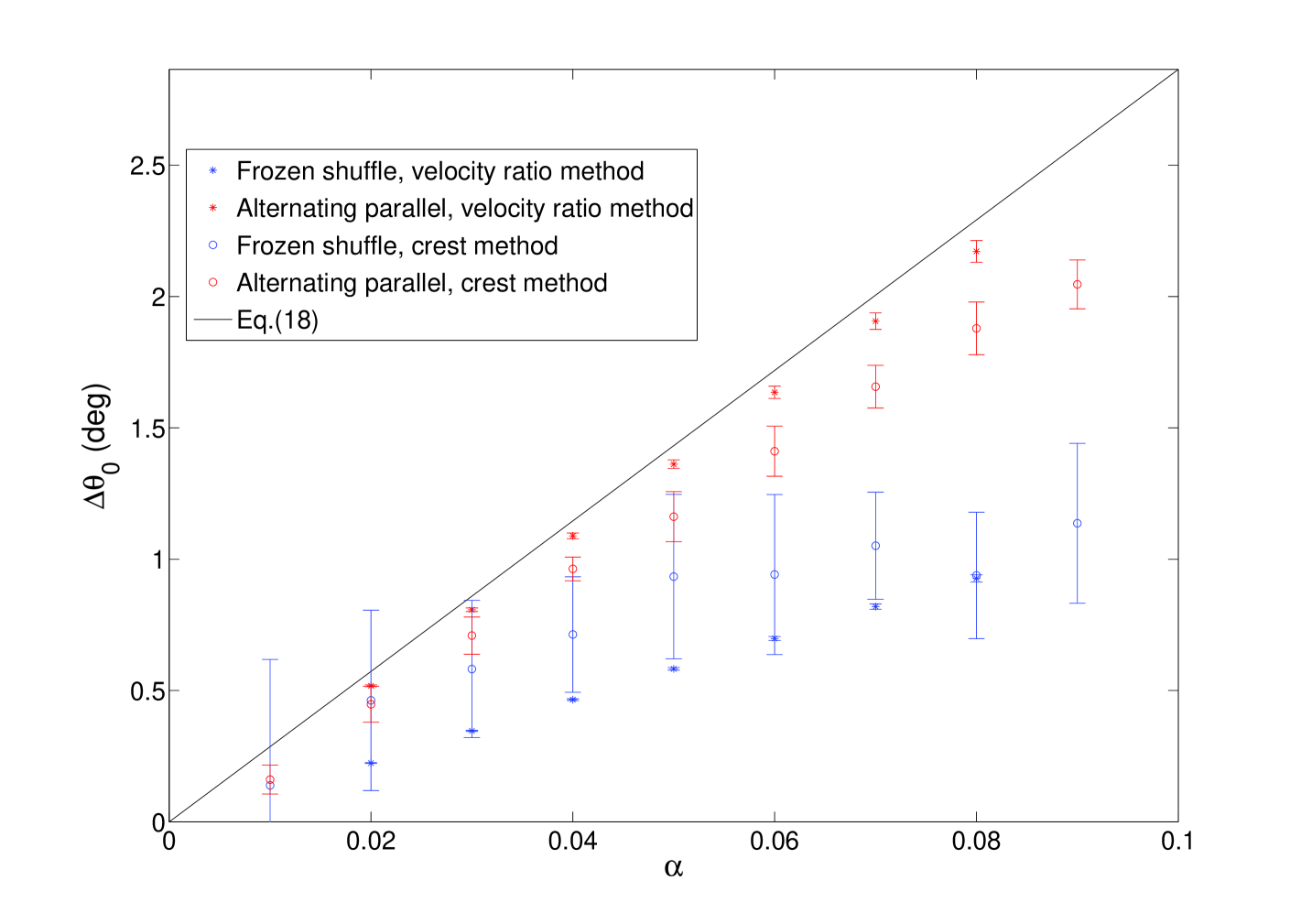
Figure 14: Chevron angle $\Delta\theta_{0}$ as a function of $\alpha$ for open boundary conditions, obtained for the two update schemes and by the two measuring methods described in section 5.3 and the two update schemes discussed in section 2.2, obtained in a system of linear size $M=640$. The solid black line corresponds to the theoretical expression (18) derived for alternating parallel update on the basis of the special class of stripes of Fig. 16.

5.3.5 The angle $\Delta\theta_{0}$

For a sequence of values of $\alpha$ we simulated a particle model having $M=640$, employing successively the two different update schemes discussed in section 2.2, and determined $\theta(\mathbf{r})$ by the two different methods discussed above. Fig. 12 shows the values for $\Delta\theta(\mathbf{r})$ obtained by the velocity ratio method. In each simulation there appear to be two triangular regions, symmetric about the diagonal and roughly coinciding with the red and dark blue regions in figure 13, where $\Delta\theta(\mathbf{r})$ is close to what appears like a limit value. We called the result of the spatial averages over these regions $\pm\Delta\theta_{0}$. The crest method was applied to the same regions and its outcome for a single particle configuration was averaged over repeated determinations at different instants of time.

The results of both methods are plotted in Fig. 14. The error bars represent the statistical standard deviation of the averaged values. It appears that in all cases there is a chevron effect and that its magnitude $\Delta\theta_{0}$ depends linearly on the control parameter $\alpha$.

In addition, numerical solution of the mean field model, not shown here, brings out a similar linear dependence of $\Delta\theta_{0}$ on the control parameter $\overline{\eta}$. Specifically, we established that

$$\Delta\theta_{0}\simeq c\alpha,\qquad\Delta\theta_{0}\simeq c^{\prime}\overline{\eta}$$ (16)

with $c\approx 12^{\circ}$ for the frozen shuffle update and $c\approx 26^{\circ}$ for the alternating parallel update in the regime $\alpha\lesssim 0.10$; while $c^{\prime}\approx 21^{\circ}$ for the mean field model in the same regime, $\overline{\eta}\lesssim 0.10$.

5.3.6 Definition of $\Delta\theta_{0}$ and limit $M\rightarrow\infty$

It is natural to ask what the stationary state will look like in the limit $M\rightarrow\infty$. However, for nonequilibrium systems like this one there appears to be little, if any, theoretical guidance to answer this question. We therefore performed particle simulations for system of very large linear sizes, up to $M=2900$, employing the alternating parallel update scheme, with the purpose of studying the behavior of the chevron angle $\Delta\theta(\mathbf{r})$ at large distances $|\mathbf{r}|$. Fig. 15 shows this angle for a system having $M=2200$ and for $\alpha=0.05$ along the line $j/i=\tan(3\pi/8)$, which bisects the upper triangular region.

The figure shows that along this line, $\Delta\theta(\mathbf{r})$ exhibits first of all a steep initial decrease with the distance from the origin. Once the penetration depth is reached, it remains confined to a narrow range around $-1.39^{\circ}$. The fluctuations around this plateau value are compatible with $\Delta\theta(\mathbf{r})$ tending to a constant along this line; however, we have no theoretical argument to exclude a very slow decay towards zero. We will therefore abstain from what one might have liked to do, namely defining $\Delta\theta_{0}$ as the $|\mathbf{r}|\to\infty$ limit of $|\Delta\theta(\mathbf{r})|$ in an appropriate direction. Instead, we will satisfy ourselves with the procedure of the preceding subsections, which amounts to identifying $\Delta\theta_{0}$ with the plateau value first reached when $|\mathbf{r}|$ exits the boundary layer.

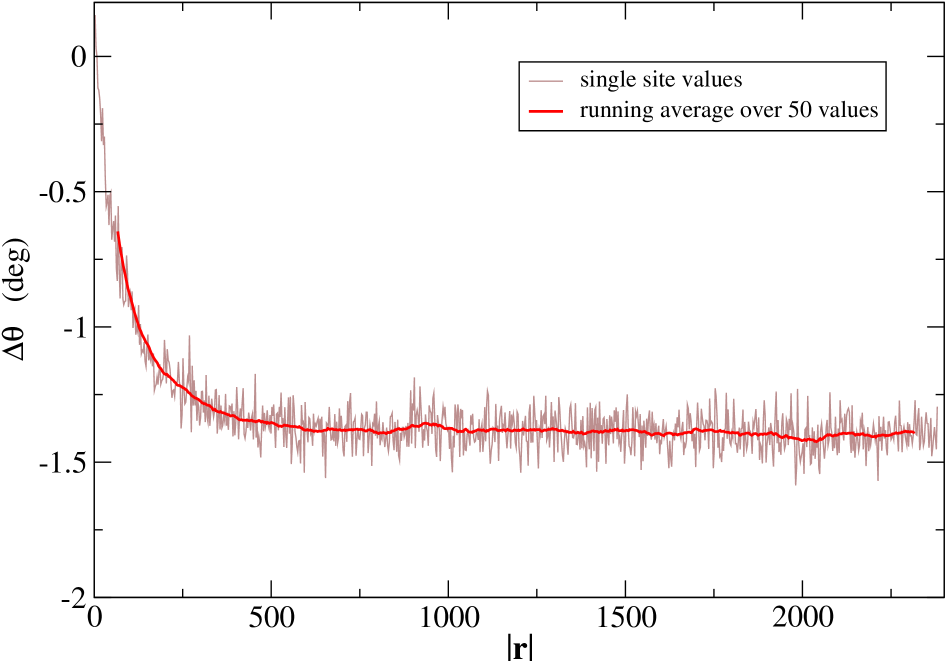
Figure 15: Chevron angle $\Delta\theta(\mathbf{r})$ determined by the velocity ratio method as a function of $|\mathbf{r}|=(i^{2}+j^{2})^{1/2}$ along the the line $j/i=\tan(3\pi/8)$, taken on one site $j$ in each column $i$, for $M=2200$ and $\alpha=0.05$, in a particle system with open boundary conditions subject to alternating parallel update. The light (brown) curve is the average over $2\times 10^{6}$ time steps after 5000 time steps have been discarded. The dark (red) curve is a running average over 50 points.

6 Chevron effect: theoretical arguments

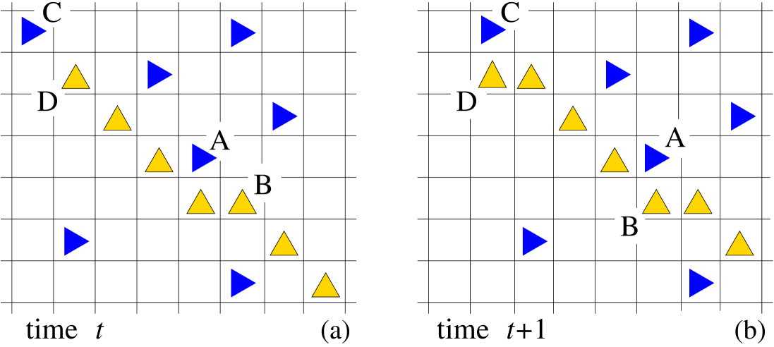
Figure 16: Mechanism causing the deviation $\Delta\theta$ of a stripe of northbound particles ( $\blacktriangle$) in the upper triangular region. The update is alternating parallel; during the time step shown first all eastbound and then all northbound particles move, provided their target site is empty.

We refer to the zoom, shown in Fig. 7, on an area located in the upper triangular region of Fig. 6. The zoom makes clear that in this region there is an important asymmetry in the spatial distribution of the eastbound and the northbound particles: the stripes of the former are dense and narrow, whereas those of the latter are sparse and wide. A consequence, visible even if barely so, is that the upper triangular region in Fig. 6 looks bluish and the lower triangle more orange-like. The asymmetry observed here offers the clue to an elementary theory of the chevron effect.

The core of the problem is to show that the system is capable of sustaining modes of propagation in which the stripes have a slope different from $45^{\circ}$. Let us consider what happens near the entrance boundary of the eastbound particles, that is, for $i\approx\xi$ but $j\gg\xi$. Near this boundary the eastbound particles ( $\blacktriangleright$), after having entered the intersection square randomly, fill the space offered to them between the northbound stripes ( $\blacktriangle$) also largely randomly. This suggests to consider the special class of northbound stripes exemplified in Fig. 16a. The stripes consist of straight segments at an angle of $45^{\circ}$, concatenated by ‘kinks’ such as the one that occurs in Fig. 16a at the level of particle B, and that is associated with the presence of the eastbound particle A. The other eastbound particles in Fig. 16a occupy random positions. Now, one time step of alternating parallel update applied to the configuration of Fig. 16a, will take it to that of Fig. 16b. This may be seen in detail as follows. We attempt to move in parallel first all eastbound and then all northbound particles. We see that during the time step from $t$ to $t+1$ none of the eastbound particles is blocked. In particular, the moves of A and C block B and D, respectively. Consequently, after the unblocked northbound particles have also moved, the kink associated with A has been displaced one lattice distance to the right along the northbound stripe, and C has created a new kink at the beginning of that stripe, at the level of particle D; this is represented in Fig. 16b. In subsequent time steps particles A and C will both travel from left to right along the stripe, each of them taking its associated kink along, and the connected structure of the stripe will be preserved.

If the set of kinks has a linear density $\rho_{\rm kink}$ along the stripe, the average stripe angle $\theta$ will be given by $\tan\theta=1-\rho_{\rm kink}$. Since $\rho_{\rm kink}$ also represents the fraction of blocked moves of the northbound particles, the stripe’s speed will be $v^{{\rm N}}=1-\rho_{\rm kink}$. By contrast, the eastbound particles move at speed $v^{{\rm E}}=1$.

In the example of Fig. 16 we note that a uniformly random spatial distribution of the particles with density $\rho^{{\rm E}}$ would lead to $\rho_{\rm kink}=\rho^{{\rm E}}$. Because $v^{{\rm E}}=1$ we have, moreover that $\rho^{{\rm E}}=J$. Using the above expressions, valid in the special situation of Fig. 16, in Eq. (12) we are led to a fully explicit expression for the angle, namely

$$\tan\theta(\mathbf{r})=1-J,$$ (17)

in which $J(\alpha)$ is given by Eq. (1), and which results in an angle $\theta$ that is independent of $\mathbf{r}$ within the region where the preceding approximations apply. To lowest order in $\Delta\theta(\mathbf{r})$ and $\alpha$ this yields, converted to degrees,

$$\Delta\theta(\mathbf{r})=\frac{\alpha}{2}\left(\frac{180}{\pi}\right)^{\circ},$$ (18)

which has been plotted in Fig. 14 as a comparison with the plateau values $\Delta\theta_{0}$. Since a correlated distribution of the eastbound particles would lead to a lower $\rho_{\rm kink}$, we expect that Eq. (17), while giving the correct order of magnitude, overestimates the slope; this is confirmed by the figure.

Hence the special class of stripes depicted in Fig. 16 demonstrates the most distinctive ingredient of the chevron effect: the existence of a nonlinear mode consisting of a stripe with an average slope different from $45^{\circ}$ and two distinct speeds of propagation, $v^{{\rm N}}<v^{{\rm E}}$. We must expect similar modes to be present for a wide class of models, including the original particle model with frozen shuffle update as well as the mean field model; for these models an explicit analysis would however be much more difficult.

In the case of the particle model we show in a complementary study [25] how an eastbound particle may get localized in the wake of another one when the two are immersed in a sea of northbound particles; the wake having the same slope as the striped mode described here.

The rule that we may derive from these considerations is the following.

Rule 1.

At the interface where a disordered species A of density $\rho_{A}$ penetrates into a perpendicular traveling and diagonally ordered species B, the speed at which the B diagonals advance is reduced from $1$ to $1-\rho_{A}$. Moreover, the (acute) angle between the diagonals and the direction of propagation of the disordered species is reduced from $\frac{\pi}{4}$ by an amount $\frac{1}{2}\rho_{A}$ (which corresponds to $\Delta\theta_{0}=\pm\frac{1}{2}\rho_{A}$, as the case may be).

7 Chevron effect on a cylinder

As shown above, the chevron effect is present for open boundary conditions (OBC) but not for periodic ones (PBC). We will now study it in the intermediate case of cylindrical boundary conditions (CBC, open for the eastbound and periodic for the northbound particles) and show that by controlling the asymmetry between the two directions we will better our understanding of the chevron effect.

An advantage of the cylindrical geometry is the translational invariance, in the statistical sense, in the vertical direction. As a consequence, by averaging the quantities of interest over the vertical coordinate, we will obtain higher precision results than for the two-way open system.

We will present this cylinder study only for the mean field model (3) and briefly comment in the end on analogous results for the particle model. For CBC the density of the northbound particles is strictly conserved in each column separately. We will set its average equal to $\overline{\rho}^{{\rm N}}$. The initial values $\rho^{{\rm N}}_{0}(\mathbf{r})$ were drawn as i.i.d. variables $\rho$ from the distribution $p(\rho;\overline{\rho}^{{\rm N}})$ of Eq. (6).

For the eastbound particles the control parameter is the average density $\overline{\eta}^{{\rm E}}$ of the boundary noise. This study therefore has the independent parameters $\overline{\eta}^{{\rm E}}$ and $\overline{\rho}^{{\rm N}}$. Fig. 17 represents a snapshot of the density fields in the stationary state for the particular set of values $\overline{\rho}^{\rm N}=0.050$ and $\overline{\eta}^{\rm E}=0.055$ on an interaction square of linear dimension $M=400$. The configuration was obtained by numerical solution of the nonlinear mean field equations (3) with CBC during $2000$ time steps; the memory of the initial state has then disappeared and the system has entered a stationary state.

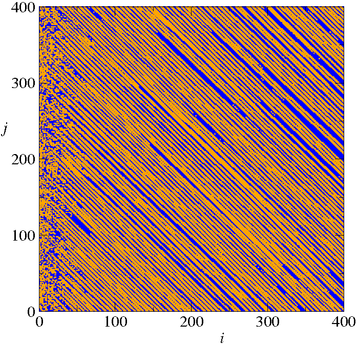
Figure 17: Snapshot representing the density fields in the intersection square of size $M=400$ and subject to cylindrical boundary conditions with control parameters $\overline{\rho}^{\rm N}=0.050$ and $\overline{\eta}^{\rm E}=0.055$. The color code is as in Fig. 8. A disordered boundary layer along the west entrance is clearly visible. The striped pattern in the bulk has an average slope of $45^{\circ}-\Delta\theta_{0}$; for the pattern shown the crest method gives $\Delta\theta_{0}\approx 1.13^{\circ}$.

7.1 Chevron effect in the stationary state

Although not easily visible to the eye, the stripes in Fig. 17 are at an angle less than $45^{\circ}$, in the way schematically shown in Fig. 1c. Along the west entrance there is a disordered boundary zone. We will now ask about the chevron angle $\Delta\theta$ as a function of the column index $i$.

Fig. 18 shows the stationary state values of  $\Delta\theta(i)$, obtained by the velocity ratio method of section 5.3.2, that is, from Eq. (12). Every curve was obtained as an average over at least 60 field configurations separated by 200 time steps to make them independent. All curves are for the same density $\overline{\rho}^{{\rm N}}=0.050$ of the northbound particles and each curve is for a different value of the boundary densities $\overline{\eta}^{{\rm E}}$ of the eastbound particles.

Fig. 18 calls for several comments. All curves show similar behavior: as $i$ increases from 1 to $M=500$, the angle $\Delta\theta(i)$ first has a narrow ‘boundary’ plateau, then a rapid decrease, and then what seems like a very wide and stable final ‘bulk’ plateau.

The first plateau corresponds to the boundary layer of width $\xi$, here equal to $\xi\approx 75$ (if we take the point of reference in the zone of rapid decrease at half the height difference between the two plateaus), independently of the value of $\overline{\eta}^{{\rm N}}$. As discussed in section 5.3.3 the values of $\Delta\theta(i)$ obtained in this boundary layer by straightforwardly applying Eq. (12), cannot be related to any angle of inclination. We can however understand the value of the boundary plateau. Near the west entrance the average density of the entering eastbound particles should equal the value imposed by the boundary condition, that is, $\langle\rho^{{\rm E}}(1)\rangle\simeq\overline{\eta}^{{\rm E}}$. When both species are uniformly distributed (which corresponds to a disordered particle system), the expected average speeds are $v^{{\rm E}}=1-\overline{\rho}^{{\rm N}}$ and $v^{{\rm N}}=1-\overline{\eta}^{{\rm E}}$ so that for $i=1$ we expect

$$\tan\Big{(}\frac{\pi}{4}+\Delta\theta(1)\Big{)}=\frac{1-\overline{\eta}^{{\rm E}}}{1-\overline{\rho}^{{\rm N}}}\,.$$ (19)

Upon expanding to linear order in $\Delta\theta(1)$ we get

$$\Delta\theta(1)=\frac{\overline{\rho}^{{\rm N}}-\overline{\eta}^{{\rm E}}}{2(1-\overline{\rho}^{{\rm N}})}\,.$$ (20)

This formula is satisfied quite well by the boundary plateau values in Fig. 18. Again, we repeat that $\Delta\theta_{0}$ does not here have the interpretation of a slope of stripes.

Of principal interest here, however, are the values of the bulk plateau. These correspond to the bulk region on the cylinder surface, where we have stripes with a single slope different from $45^{\circ}$, rather than chevrons. We will nevertheless continue to speak of the ‘chevron effect’ in this case, too. Actually, in the bulk $\Delta\theta(i)$ seems to show a very slight increase with $i$, as is clear in particular for the smaller values of $\overline{\eta}^{{\rm E}}$. In order to arrive at a unique value for $\Delta\theta_{0}$ we determined $\Delta\theta_{0}$ as the average of $|\Delta\theta(i)|$ over the columns with $200\leq i\leq 300$, then averaged over at least 60 determinations. The results are represented by the red square dots in Fig. 19.

Along with the velocity ratio method we applied to the same field configurations also the crest method. The results are represented by the black round dots in the same figure.

The error bars for each method are of the order of the symbol size; they were estimated from variances obtained by dividing the data for each data point into five subsets. The results of the two methods are sufficiently close that we may speak of a coherent picture. They are nevertheless clearly distinct: the error bars do not overlap. One factor that may contribute to this difference is the fact that Eq. (14) is valid only for stripes that are mutually impenetrable, a condition that is not necessarily fully satisfied in the model.

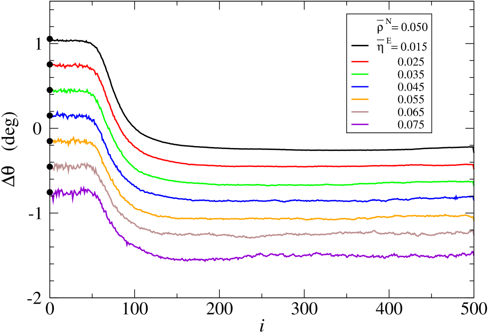
Figure 18: Chevron angle $\Delta\theta$ as a function of the column index $i$, obtained by simulation of the mean field equations (3) and measured by means of the velocity ratio method, on a square lattice of linear size $M=500$ with cylindrical boundary conditions. The northbound particles have a fixed density $\overline{\rho}^{\rm N}=0.050$. Curves are shown for various boundary densities $\overline{\eta}^{\rm E}$ of the eastbound particles. The dots for $i=1$ are the boundary values predicted by Eq. (20).

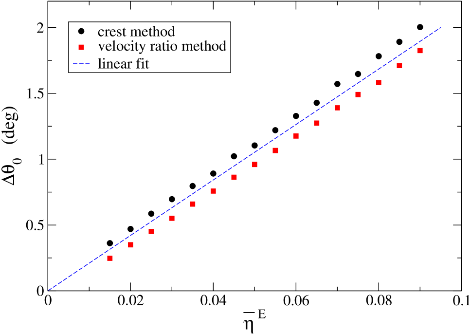
Figure 19: Chevron angle $\Delta\theta_{0}$ as a function of the average density $\overline{\eta}^{{\rm E}}$ imposed at the open west boundary and for fixed $\overline{\rho}^{\rm N}=0.050$, obtained by simulation of the mean field equations (3) and measured by both the crest and the velocity ratio method, on a square lattice of linear size $M=500$ with cylindrical boundary conditions. The error bars are of the same order as the symbols. The straight line through the origin is the closest fit to both data sets; it has a slope of $21^{\circ}$.

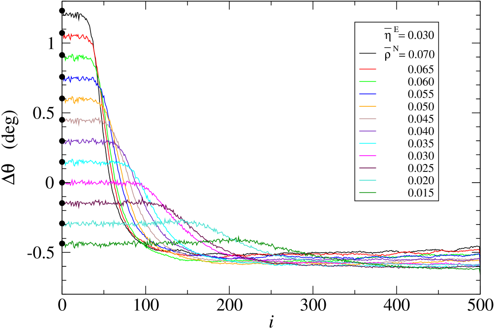
Figure 20: Chevron angle $\Delta\theta$ as a function of the column index $i$, obtained by simulation of the mean field equations (3) and measured by means of the velocity ratio method, on a square lattice of linear size $M=500$ with cylindrical boundary conditions. The eastbound particles have a fixed boundary density $\overline{\eta}^{{\rm E}}=0.030$. Curves for various densities $\overline{\rho}^{{\rm N}}$ of the northbound particles show different penetration depths $\xi$ but have closely similar plateau values for $i\gtrsim\xi$. The dots for $i=1$ are the boundary values predicted by Eq. (20).

Fig. 20 shows another set of curves of the column dependent chevron angle, obtained in the same way as those of Fig. 18, but now all curves are for the same $\overline{\eta}^{{\rm E}}=0.030$ and each one is for a different value of $\overline{\rho}^{{\rm N}}$. It appears that all these curves have plateau values $-\Delta\theta_{0}$ with $0.50^{\circ}\lesssim\Delta\theta_{0}\lesssim 0.60^{\circ}$. which is fully compatible with the data point of Fig. 19 for $\overline{\eta}^{{\rm E}}=0.030$, namely $\Delta\theta_{0}=0.55^{\circ}\pm 0.02^{\circ}$. There is however a slight drift of the plateau value with increasing $i$. This effect becomes more pronounced as $\overline{\eta}^{{\rm E}}$ gets larger but we have not pursued our investigation of this point. We notice that the values $\Delta\theta(1)$ are again in perfect agreement with Eq. (20). Finally, Fig. 20 shows the variation of the width of the boundary layer with $\overline{\rho}^{{\rm N}}$. If we let again the points at mid-height between the boundary plateau and the bulk plateau determine the penetration depth $\xi$, a crude fit shows that $\xi\approx 4.2/\overline{\rho}^{{\rm N}}$ for $\overline{\rho}^{{\rm N}}\to 0$.

The cylinder study described here was carried out for the mean-field model of Eqs. (3). Similar results for the particle model, not reported here, show that in that system, too, the chevron angle is linear in the density of the eastbound particles and independent of the density of the northbound ones. In each case the explanation lies in the asymmetry caused by the fact that the entering particle species is fully disordered whereas the other species has had time to organize.

These density dependencies are the main result of our investigation with CBC boundary conditions.

7.2 Chevron effect in a transient

The system to be studied in this final section has been designed for the sole purpose of testing our understanding of the chevron effect. Whereas until now we dealt exclusively with stationary state properties, we will here consider a transient  effect, and that for a very particular set of initial conditions. We consider again the mean field equations (3) in cylindrical geometry and prepare the system at time $t=0$ in a state with the uniform nonrandom initial condition $\rho^{{\rm E}}_{0}(\mathbf{r})=\rho^{{\rm N}}_{0}(\mathbf{r})=\overline{\rho}_{0}$. This initial state would be stationary if there were no open boundaries. We however evolve this system in time with the same random density boundary condition as before along the west entrance, characterized by an $\overline{\eta}^{{\rm E}}$, and with free exit at the east boundary.

We considered specifically a system of linear size $M=500$ having $\overline{\rho}^{{\rm N}}=\overline{\eta}^{{\rm E}}=\overline{\rho}_{0}=0.10$. At time $t=400$, the stationary state has not set in yet. A density plot of the fields then looks like in Fig. 21. In Fig. 22 we show the corresponding column dependent values of the chevron angle $\Delta\theta(i)$. These figures call for the following comments.

We now discuss Fig. 21 and Fig. 22 in the order of decreasing column index. Since the influence from the boundary penetrates into the bulk by one lattice unit per time step, at time $t=400$ the region of the intersection square with column index $i\geq 400$, colored gray in the figure, has remained in the initial uniform state. In the region $325\lesssim i<400$ the amplitude of the perturbation decays exponentially; we will discuss this zone in greater detail in another article [24].

Of main interest is the region $50\lesssim i\lesssim 325$, which has the diagonally striped structure characteristic of the crossing flows. The region consists of two zones, I and II, extending between $50\lesssim i\lesssim 175$ and $200\lesssim i\lesssim 325$, respectively. Although barely visible in Fig. 21, the stripes in the zones I and II have different angles of inclination $\theta$. This becomes very clear in Fig. 22, which shows the chevron angle $\Delta\theta(i)=\theta(i)-\frac{\pi}{4}$ as a function of the column index $i$. In zones I and II this angle has two distinct plateau values close to $\mp\Delta\theta_{0}$, respectively, where $\Delta\theta_{0}=2.0^{\circ}$. The two zones are separated by a transition layer and zone I is separated from the boundary by the usual boundary layer.

During the time evolution the widths of zones I and II increase roughly linearly with $t$ whereas the transition layer keeps a constant width. Hence zone I gradually extends all the way to the east end of the interaction square and forces zone II (and with it one leg of the chevron) out of the system. What remains is a stationary state of the type studied in section 7.1, with a value $-\Delta\theta_{0}=-2.0^{\circ}$ for the chevron angle.

The appearance during the transient of a zone II with the opposite value of the chevron angle needs to be explained. The explanation follows from rule 1 (section 6). In the present case, at the right hand interface of zone II the northbound particles constitute the disordered species which invades the eastbound ones that are diagonally ordered. Therefore, according to the rule, the angle between the diagonals and the direction of propagation of the disordered species (which here moves northward) is reduced by $\frac{1}{2}\overline{\rho}^{{\rm N}}$; and Fig. 22 shows exactly that effect. The difference with what happens at the entrance boundary is that here the ordered species moves perpendicular to the interface and the disordered one parallel to it.

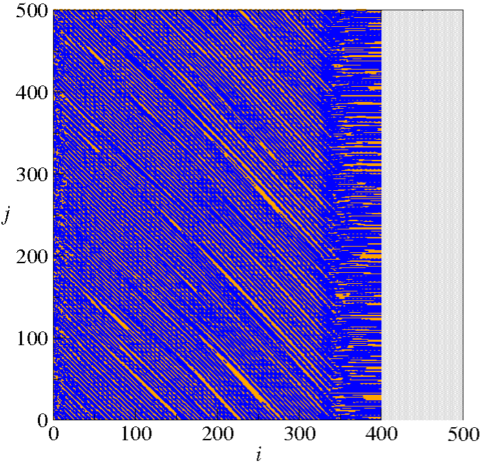
Figure 21: Density field showing the transient configuration at time $t=400$ on an intersection square of linear size $M=500$ with cylindrical boundary conditions. The color code is as in Fig. 8. The west entrance boundary is subject to a random boundary density of average $\overline{\eta}^{{\rm E}}=0.10$. The nonrandom initial condition was $\rho^{{\rm E},{\rm N}}_{0}(\mathbf{r})=0.10$. In the grey area these initial values still persist at time $t=400$.

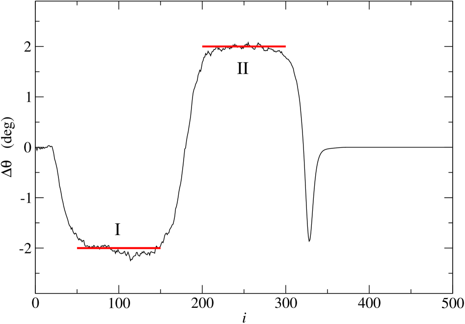
Figure 22: Chevron angle $\Delta\theta$ as a function of the column index $i$, determined by the velocity ratio method in the configuration of Fig. 21. The heavy horizontal red lines mark the plateau values $\pm 2^{\circ}$.

8 Summary and conclusion

We have considered in this work a class of theoretical models of two crossing unidirectional traffic flows, one composed of eastward and one of northward traveling particles. The basic model parameters are the street width $M$ and either the imposed current or the imposed particle density. Because of their simplicity, we believe that this class of models has an intrinsic interest as an example of a driven nonequilibrium system.

We have discussed a phenomenon observed widely in more realistic many-parameter models as well as in experiments [26], namely the instability – in the crossing area – of the randomly uniform state against segregation into diagonal stripes of alternatingly northward and eastward traveling species. We have shown that during the development of the instability the particles of each species aggregate into string-like structures.

The principal models in our class are a particle model with two different update rules and a closely related mean field model. The latter has allowed us to provide an analytic explanation of the instability in the simplest possible context, namely when the two flows go around a torus. Such toroidal geometry has become popular since the introduction of the BML model [12]. The linear stability analysis that we performed for the torus may be extended to the open intersection square; that calculation is however very cumbersome and will be the subject of a future publication [24].

We have moreover discovered that for a crossing with open boundary conditions, which is the case of principal interest in this work, the stripes actually have two branches that join to form a chevron. The slopes of the branches (with respect to the two flow directions) differ from $45^{\circ}$ by an amount $\pm\Delta\theta_{0}$ that we call the chevron angle. The angle is negative in the upper triangular half of the intersection square and positive in the lower half. Its absolute value is very small (less than $2^{\circ}$ in all cases studied), but the chevron effect is robustly present in all model versions that we studied. We found by simulation that $\Delta\theta_{0}$ is linear in the density of the particles coming in through a boundary, and independent of the density of the particles moving parallel to that boundary.

The chevron phenomenon disappears in the limit of zero particle density for two different reasons. First of all, the chevron angle becomes small, and secondly, the boundary layer of width $\xi$ beyond which it is visible, extends further and further into the system. So we cannot study the chevron effect in the limit $\rho\to 0$ in finite systems, and in this sense the effect is nonperturbative.

In section 6 we provided some elementary theoretical arguments that explain the chevron effect and that involve the formation of linear aggregates (stripes) of same-type particles. We obtained an approximate but explicit formula for the chevron angle as a function of the particle density.

The theory is based on the special limiting situation in which one particle type is fully aggregated into strings and the other one randomly and uniformly distributed in space, an asymmetry indeed clearly observed in the simulations. One may nevertheless consider that the theory of the chevron effect still needs further development. It is tempting to speculate that there exists a hydrodynamic theory with two components each of which is characterized not only by its average local density and velocity, but also by a variable expressing its degree of aggregation. In future work [25] we will return to related questions and study the interaction between two particles traveling on parallel lanes, as mediated by a sea of perpendicular particles.

The various different manifestations of the stripe formation instability and the chevron effect studied above point to the conclusion that these phenomena occur generically whenever we have crossing unidirectional flows with hard core interaction and deterministic rules of motion.

Further questions that may be asked concern modifications of the model. What happens, for example, if blocked particles are allowed to jump laterally? What happens if, for open boundary conditions, the two directions have different imposed flow rates? Furthermore, from a theoretical point of view the $M\to\infty$ limit of this system is interesting. As far as we have been able to ascertain, the ‘chevron’ states that we discovered are stable stationary states, but we are not sure what they become in the infinite system limit. A related question concerns the behavior in an anisotropic geometry, that is, in an $M_{1}\times M_{2}$ intersection rectangle where one side of the rectangle might tend to infinity with the other one fixed.

Some of these questions will be the subject of future work.

References

- [1] A. Schadschneider, Modelling of transport and traffic problems, Lecture Notes in Computer Science 5191 (2008) 22–31.
- [2] D. Helbing, Traffic and related self-driven many-particle systems, Reviews of Modern Physics 73 (2001) 1067–1141.
- [3] M. C. Cross, P. C. Hohenberg, Pattern formation outside of equilibrium, Rev. Mod. Phys. 65 (1993) 851–1108.
- [4] S. Wolfram, Statistical mechanics of cellular automata, Rev. Mod. Phys. 55 (1983) 601–644.
- [5] N. Packard, S. Wolfram, Two-dimensional cellular automata., J. Stat. Phys. 38 (1985) 901–946.
- [6] S. Wolfram, Universality and complexity in cellular automata., Physica D 10 (1984) 1–35.
- [7] K. Nagel, M. Schreckenberg, A cellular automaton model for freeway traffic, J. Physique I 2 (1992) 2221–2229.
- [8] M. E. Fouladvand, Z. Sadjadi, M. R. Shaebani, Optimized traffic flow at a single intersection: traffic responsive signalization, J. Phys. A: Math. Gen. 37 (2004) 561–576.
- [9] M. E. Foulaadvand, M. Neek-Amal, Asymmetric simple exclusion process describing conflicting traffic flows, EPL 80.
- [10] H.-F. Du, Y.-M. Yuan, M.-B. Hu, R. Wang, R. Jiang, Q.-S. Wu, Totally asymmetric exclusion processes on two intersected lattices with open and periodic boundaries, J. Stat. Mech. (2010) P03014.
- [11] C.Appert-Rolland, J.Cividini, H.J.Hilhorst, Intersection of two tasep traffic lanes with frozen shuffle update, J. Stat. Mech. (2011) P10014.
- [12] O. Biham, A. Middleton, D. Levine, Self-organization and a dynamic transition in traffic-flow models, Phys. Rev. A 46 (1992) R6124–R6127.
- [13] Z.-J. Ding, R. Jiang, B.-H. Wang, Traffic flow in the biham-middleton-levine model with random update rule, Phys. Rev. E 83 (2011) 047101.
- [14] Z.-J. Ding, R. Jiang, W. Huang, B.-H. Wang, Effect of randomization in the biham–middleton–levine traffic flow model, J. Stat. Mech. (2011) P06017.
- [15] S. Hoogendoorn, P. H. Bovy, Simulation of pedestrian flows by optimal control and differential games, Optim. Control Appl. Meth. 24 (2003) 153–172.
- [16] M. Moussaïd, E. Guillot, M. Moreau, J. Fehrenbach, O. Chabiron, S. Lemercier, J. Pettré, C. Appert-Rolland, P. Degond, G. Theraulaz, Traffic instabilities in self-organized pedestrian crowds, PLoS Computational Biology 8 (2012) 1002442.
- [17] B. Schmittmann, R. Zia, Statistical Mechanics of driven diffusive systems, Vol. 17 of Phase Transitions and Critical Phenomena, Academic Press, New York, 2013.
- [18] J. Dzubiella, G. P. Hoffmann, H. Löwen, Lane formation in colloidal mixtures driven by an external field, Phys. Rev. E 65 (2002) 021402.
- [19] K. Yamamoto, M. Okada, Continuum model of crossing pedestrian flows and swarm control based on temporal/spatial frequency, in: 2011 IEEE International Conference on Robotics and Automation, 2011.
- [20] H. Hilhorst, C. Appert-Rolland, A multi-lane TASEP model for crossing pedestrian traffic flows, J. Stat. Mech. (2012) P06009.
- [21] J. Cividini, C. Appert-Rolland, H. Hilhorst, Diagonal patterns and chevron effect in intersecting traffic flows, Europhys. Lett. 102 (2013) 20002.
- [22] C.Appert-Rolland, J. Cividini, H.J.Hilhorst, Frozen shuffle update for an asymmetric exclusion process on a ring, J. Stat. Mech. (2011) P07009.
- [23] C.Appert-Rolland, J.Cividini, H.J.Hilhorst, Frozen shuffle update for an asymmetric exclusion process with open boundary conditions, J. Stat. Mech. (2011) P10013.
- [24] J. Cividini, H. Hilhorst, In preparation.
- [25] J. Cividini, C. Appert-Rolland, Wake-mediated interaction between driven particles crossing a perpendicular flow, arXiv:1305.3206.
- [26] S. P. Hoogendoorn, W. Daamen, Self-organization in walker experiments, in: S. Hoogendoorn, S. Luding, P. Bovy, et al. (Eds.), Traffic and Granular Flow ’03, Springer, 2005, p. ??