Modeling the Infrared Extinction toward the Galactic Center

Abstract

We model the ${\sim}\,$1–19$\,{\rm\mu m}$ infrared (IR) extinction curve toward the Galactic Center (GC) in terms of the standard silicate-graphite interstellar dust model. The grains are taken to have a power law size distribution with an exponential decay above some size. The best-fit model for the GC IR extinction constrains the visual extinction to be ${A_{\rm V}}$ ${\sim}\,$38–42$\,{\rm mag}$. The limitation of the model, i.e., its difficulty in simultaneously reproducing both the steep ${\sim}\,$1–3$\,{\rm\mu m}$ near-IR extinction and the flat ${\sim}\,$3–8$\,{\rm\mu m}$ mid-IR extinction is discussed. We argue that this difficulty could be alleviated by attributing the extinction toward the GC to a combination of dust in different environments: dust in diffuse regions (characterized by small ${R_{\rm V}}$ and steep near-IR extinction), and dust in dense regions (characterized by large ${R_{\rm V}}$ and flat UV extinction).

1 Introduction

The wavelength dependence of the interstellar extinction – known as the “interstellar extinction law (or curve)” – is one of the primary sources of information about the interstellar grain population (Draine 2003). The Galactic interstellar extinction curves in the ultraviolet (UV) and visual wavelengths vary from one sightline to another, and can be parameterized in terms of the single parameter ${R_{\rm V}}\equiv{A_{\rm V}}/E(B-V)$, the total-to-selective extinction ratio (Cardelli et al. 1989). Larger values of ${R_{\rm V}}$ correspond to size distributions skewed toward larger grains (e.g., dense clouds tend to have large values of ${R_{\rm V}}>4$). On average, the dust in the diffuse interstellar medium (ISM) corresponds to ${R_{\rm V}}\approx 3.1$.

However, the infrared (IR) interstellar extinction law, which also varies from sightline to sightline, cannot be simply represented by ${R_{\rm V}}$. Various recent studies have shown that there does not exist a “universal” near-IR (NIR) extinction law (Fitzpatrick & Massa 2009; Gao et al. 2009; Zasowski et al. 2009) and the mid-IR (MIR) extinction law shows a flat curve and lacks the model-predicted pronounced minimum extinction around 7$\,{\rm\mu m}$ (Draine 1989). It is worth noting that the flat MIR extinction curves determined for various sightlines all appear to agree with the extinction predicted by the standard silicate-graphite interstellar grain model for ${R_{\rm V}}$ = 5.5 (Weingartner & Draine 2001) (hereafter WD01), which indicates a dust size distribution favoring larger sizes compared to that for ${R_{\rm V}}=3.1$.

Recently, using the hydrogen emission lines of the minispiral observed by ISO-SWS and SINFONI, Fritz et al. (2011) derived the IR extinction curve toward the inner GC from 1 to 19$\,{\rm\mu m}$. The extinction curve shows a steep NIR extinction consistent with that of Nishiyama et al. (2006, 2009) and a flat MIR extinction consistent with other sightlines (see Figure 1). It differs from the IR extinction law toward the GC derived by Rieke & Lebofsky (1985) (hereafter RL85) and Rieke et al. (1989). Based on their observations, Fritz et al. (2011) argued that the extinction at the visual band (${A_{\rm V}}$) toward the GC may be as high as ${A_{\rm V}}$ ${\sim}\,$59$\,{\rm mag}$ (with the exact ${A_{\rm V}}$ depending on the chosen gas-to-dust ratio $N_{\rm H}/{A_{\rm V}}$), much larger than ${A_{\rm V}}\sim 31$ estimated by Rieke et al. (1989) which is commonly adopted in the astronomical literature.

In this work, we try to use the standard interstellar grain model which consists of graphite and silicate grains (Draine & Lee 1984) to fit the observed IR extinction curve toward the GC of Fritz et al. (2011) and constrain the total optical extinction (${A_{\rm V}}$) toward the GC. §2 briefly describes the grain model. Our model results are presented in §3 and discussed in §4. In §5 we summarize the major conclusion of this work.

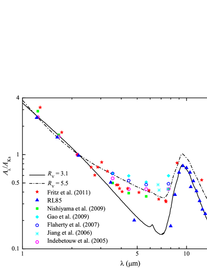
Figure 1: IR extinction laws compiled from the literature. Red stars plot $A_{\lambda}/A_{\rm K_{s}}$ toward the GC based on H lines (Fritz et al. 2011). Blue triangles are derived from stars toward the GC (RL85). Green squares are derived from the red clump giants toward the GC (Nishiyama et al. 2009). Cyan diamonds are the Galactic plane average extinction at $|l|<5^{\circ}$ and $|b|<2^{\circ}$ (Gao et al. 2009). The other three kinds of symbols plot the extinction laws obtained from sightlines away from the GC. For comparison, the extinction curves calculated from the interstellar grain model (WD01) for ${R_{\rm V}}=3.1$ (black solid line) and ${R_{\rm V}}=5.5$ (black dot-dashed line) are also shown.

2 Dust Model

We take the dust to be a mixture of separate amorphous silicate and graphite grains, with the optical properties taken from Draine & Lee (1984). For the dust size distribution, we adopt a power law with an expoential cutoff at some large size: $dn/da=A\,n_{\rm H}\,a^{-\alpha}\exp\left(-a/a_{\rm b}\right)$ with $50\,{\rm\AA}<a<1\,{\rm\mu m}$, where $a$ is the grain radius, $dn$ is the number density of dust with radii in the interval [$a$, $a$ $+$ $da$] per H nuclei, $n_{\rm H}$ is the number density of H nuclei, $A$ is the normalization constant, $\alpha$ is the power index, and $a_{\rm b}$ is the cutoff size. In our modeling, we will have six parameters: $A_{\rm si}$, $\alpha_{\rm si}$, $a_{\rm b,si}$ for the silicate component, and $A_{\rm c}$, $\alpha_{\rm c}$, $a_{\rm b,c}$ for the graphite component. The total extinction at wavelength $\lambda$ is given by

$$A_{\lambda}=(2.5\log e)N_{\rm H}\sum_{i}\int da\frac{dn_{i}(a)}{da}C_{{\rm ext},i}(a,\lambda),\\$$ (1)

where the summation is made over the two grain types (i.e., silicate and graphite), $N_{\rm H}\equiv\int n_{\rm H}\,dl$ is the H column density which is the H number density integrated over the line of sight $l$, and $C_{{\rm ext},i}(a,\lambda)$ is the extinction cross section of grain type $i$ of size $a$ at wavelength $\lambda$. The goodness of fitting is evaluated by

$$\frac{\chi^{2}}{\rm d.o.f}=\frac{\sum_{j=1}^{N_{\rm obs}}\left(A_{\lambda}^{\rm mod}-A_{\lambda}^{\rm obs}\right)^{2}/\sigma_{j}^{2}}{N_{\rm obs}-N_{\rm para}}~{}~{},$$ (2)

where $A^{\rm obs}_{\lambda}$ is the IR extinction toward the GC derived by Fritz et al. (2011) (see their Table 2), $N_{\rm obs}$ is the number of observational data points, $N_{\rm para}$ is the number of adjustable parameters ($N_{\rm para}=6$ if we assume different size distributions for silicate and graphite; $N_{\rm para}=4$ if we assume that both dust components have the same size distribution), $A^{\rm mod}_{\lambda}$ is the model extinction computed from eq.1, and $\sigma_{j}$ is the weight of the observed extinction.

Assuming that $\approx$30% is in the gas phase, WD01 adopt the solar abundance of Grevesse & Sauval (1998) to constrain their models. Their CASE A models tried to seek the best fit by varying the total volume per H in both the carbonaceous and silicate distributions, while their CASE B models fixed at approximately the values found for ${R_{\rm V}}=3.1$. Following WD01, we fix the total dust quantity (per H nuclei) to be consistent with the cosmic abundance constraints. Let $V_{\rm tot,si}$ be the total volume of the silicate dust, and $V_{\rm tot,c}$ be the total volume of the graphitic dust. We take $V_{\rm tot,si}=2.98\times 10^{-27}\rm\,cm^{3}\,H^{-1}$ and $V_{\rm tot,c}=2.07\times 10^{-27}\rm\,cm^{3}\,H^{-1}$ (i.e., values for constraining all “CASE A” models of WD01). We will also consider $V_{\rm tot,si}=3.9\times 10^{-27}\rm\,cm^{3}\,H^{-1}$ and $V_{\rm tot,c}=2.3\times 10^{-27}\rm\,cm^{3}\,H^{-1}$ (i.e., fixed values for all “CASE B” models of WD01). The mass densities of amorphous silicate and graphite are taken to be $\rho_{\rm sil}\approx 3.5\,{\rm g}\,{\rm cm}^{-3}$ and $\rho_{\rm carb}\approx 2.24\,{\rm g}\,{\rm cm}^{-3}$.

Table 1: Model parameters for fitting the GC IR extinction curve

Abundance	$dn/da$		$\chi^{2}/{\rm d.o.f}$	${A_{\rm V}}$	$A_{\rm Ks}$	${R_{\rm V}}$	$N_{\rm H}$
	silicate	graphite					$\times 10^{22}\rm cm^{-2}$
Fitting the observed extinction curve from 1$\,{\rm\mu m}$ to 19$\,{\rm\mu m}$a
CASE A	$a^{-2.4}e^{-a/0.04}$		21.3/14	39.93	2.81	2.23	7.5
CASE B	$a^{-2.6}e^{-a/0.05}$		20.4/14	38.38	2.79	2.34	7.2
CASE A	$a^{-3.1}e^{-a/0.10}$	$a^{-2.7}e^{-a/0.04}$	17.2/12	40.57	2.71	2.31	7.6
CASE B	$a^{-2.9}e^{-a/0.08}$	$a^{-2.5}e^{-a/0.04}$	17.0/12	41.28	2.69	2.34	7.7
Only fitting the observed extinction from 1$\,{\rm\mu m}$ to 7$\,{\rm\mu m}$
CASE B	$a^{-3.0}e^{-a/0.09}$	$a^{-3.1}e^{-a/0.04}$	10.5/9	39.93	2.40	2.12	7.5
CASE B with AMC	$a^{-3.1}e^{-a/0.12}$	$a^{-3.0}e^{-a/0.06}$	10.4/9	35.70	2.55	2.50	6.7
Only fitting the observed extinction from 3$\,{\rm\mu m}$ to 19$\,{\rm\mu m}$
CASE B	$a^{-4.0}e^{-a/0.03}$	$a^{-3.1}e^{-a/0.02}$	10.6/9	30.84	3.04	1.77	5.8
CASE B with AMC	$a^{-3.8}e^{-a/0.02}$	$a^{-3.3}e^{-a/0.03}$	11.7/9	19.26	3.01	2.19	3.6
Fitting with combinations of multi-extinction curves (see $\S$4.3)
$f_{{R_{\rm V}}=2.1}$	$f_{{R_{\rm V}}=3.1}$	$f_{{R_{\rm V}}=5.5}$	$\chi^{2}/{\rm d.o.f}$	${A_{\rm V}}$	$A_{\rm Ks}$	${R_{\rm V}}$
0.30	0.49	0.21	39.1/14	34.56	2.66	2.60
0.28	0.39	0.33b	40.7/15	33.67	2.63	2.70
aWe only consider 18 of 21 points of Fritz et al. (2011) in order to reduce the effect of the 3.1$\,{\rm\mu m}$ H2O feature. bMcFadzean et al. (1989) argued that the molecular clouds may contribute as much as ${\sim}\,$1/3 ($\sim$10 mag) of the total visual extinction ${A_{\rm V}}$ towards the GC. Therefore, we fixed the fraction of the ${R_{\rm V}}=5.5$-type extinction to be 0.33.

3 Model Extinction

To testify the dust model, we first fit the standard extinction curve of ${R_{\rm V}}=3.1$. With $dn/da\propto a^{-3.5}e^{-a/0.14}$ for amorphous silicates and $dn/da\propto a^{-3.1}e^{-a/0.11}$ for graphite, the model closely reproduces the ${R_{\rm V}}=3.1$ Galactic extinction curve. To fit the observed IR extinction curve from 1$\,{\rm\mu m}$ to 19$\,{\rm\mu m}$ toward the GC (Fritz et al. 2011), for simplicity we first assume that both graphite and silicate have the same size distribution (i.e. $\alpha_{\rm si}=\alpha_{\rm c}$, $a_{\rm b,si}=a_{\rm b,c}$). We then consider models with different power indices and cutoff sizes for the two dust components to search for better fits. The best-fit results are summarized in Table 1. We note that it makes little difference either taking the same size distribution or assuming different size distributions for silicate and graphite. None of these attempts could fit the flat MIR extinction well, although “CASE B” works relatively better.

In Figure 2 we show the “CASE B” best-fit model extinction assuming different size distributions for silicate and graphite. Compared with the observed IR extinction curve toward the GC (Fritz et al. 2011), the model extinction is too high at the 2.166$\,{\rm\mu m}$ (Brackett-$\gamma$) band and too low at ${\sim}\,$7$\,{\rm\mu m}$: $A_{2.166}^{\rm mod}\approx 2.68\,{\rm mag}$ while Fritz et al. (2011) obtained $A_{2.166}\approx 2.49\pm 0.11\,{\rm mag}$. The size distribution of $\alpha_{\rm c}\approx-2.5$ and $a_{\rm b,c}\approx 0.04\,{\rm\mu m}$ for graphite reproduces well the steep NIR extinction but causes the minimum extinction near $7\,{\rm\mu m}$. The small cutoff $a_{\rm b,c}\approx 0.04\,{\rm\mu m}$ implies that the model is rich in small graphite grains so that the model extinction curve is similar to that of ${R_{\rm V}}=2.1$ in the UV. The size distribution of $\alpha_{\rm si}\approx-2.9$ and $a_{\rm b,si}\approx 0.08\,{\rm\mu m}$ for silicate causes the strong silicate feature at 9.7$\,{\rm\mu m}$. Our results show that it may require some dust grains with a size distribution peaking around 0.5$\,{\rm\mu m}$ or even larger to produce the flat MIR extinction. To avoid the complication of the silicate features we have also modeled the observed extinction but limiting ourselves to the extinction from 1$\,{\rm\mu m}$ to $7\,{\rm\mu m}$. To fit the MIR extinction, we have also tried models confining us to the observed extinction from 3$\,{\rm\mu m}$ to 19$\,{\rm\mu m}$ (i.e., ignoring the 1–3$\,{\rm\mu m}$ NIR extinction). These approaches seem to work well for the chosen wavelength range, but unfortunately, none of these attempts results in satisfactory fits for the whole range of 1-19$\,{\rm\mu m}$. Finally, we replace graphite by amorphous carbon (AMC). But we are still not able to simultaneously fit both the NIR and MIR extinction.

The NIR extinction law toward the GC derived by Fritz et al. (2011) and Nishiyama et al. (2009) is much steeper than that derived by Rieke & Lebofsky (1985) and Rieke et al. (1989), with $\beta\approx-2.0$ compared to the common value of $\beta\approx-1.6$ to $-1.8$. For comparison, we also fit the extinction curve of Rieke et al. (1989) , which is actually the ${R_{\rm V}}=3.1$-type extinction, and the model also works very well with $dn/da\propto a^{-2.1}e^{-a/0.08}$ for amorphous silicates and $dn/da\propto a^{-3.0}e^{-a/0.28}$ for graphite. For the sake of clear comparison, we replot in Figure 3 the results shown in Figure 2 but in terms of $A_{\lambda}/{A_{\rm V}}$. We see that the IR extinction toward the GC derived by Fritz et al. (2011) seems to be a combination of the steep UV-to-NIR extinction of ${R_{\rm V}}=2.1$, the flat MIR extinction of ${R_{\rm V}}=5.5$, and the strong silicate feature of ${R_{\rm V}}=3.1$. It seems that a trimodal size distribution is required in order to achieve a close fit to the observed extinction from the UV through NIR, MIR to the silicate absorption band.

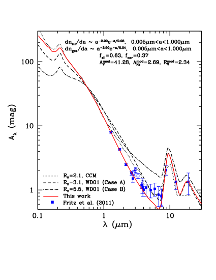
Figure 2: Comparison of the model extinction curve (red solid line) with the ${\sim}\,$1–19$\,{\rm\mu m}$ IR extinction of the GC (blue squares) observed by Fritz et al. (2011). Also shown are the extinction curves of ${R_{\rm V}}=2.1$ (dotted line, see Cardelli et al. (1989)), ${R_{\rm V}}=3.1$ (dashed line, WD01) and ${R_{\rm V}}=5.5$ (dot-dashed line, WD01) with the silicate absorption features added (Draine 2003).

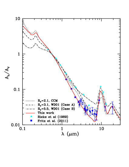
Figure 3: Same as Figure 2 but with the y-axis plotted as $A_{\lambda}/{A_{\rm V}}$. The GC IR extinction curve of Fritz et al. (2011) is normalized to ${A_{\rm V}}=42\,{\rm mag}$ (blue squares). Also shown is the GC extinction of Rieke et al. (1989) (Cyan triangles), taking ${A_{\rm V}}=31\,{\rm mag}$.

4 Discussion

4.1 The Extinction Features in the 3–7$\,{\rm\mu m}$ Wavelength Range

The extinction curve toward the GC obtained by Fritz et al. (2011) shows the strong $3.1\,{\rm\mu m}$ $\rm H_{2}O$ feature and the 3.4$\,{\rm\mu m}$ aliphatic hydrocarbon feature. Fritz et al. (2011) found that the COMP-AC-S model of Zubko et al. (2004) seems to best fit their observations as judged by $\chi^{2}/{\rm d.o.f.}$ and the presence of the H₂O ice features. The porosity of ice dust grains also makes Zubko et al. (2004)’s extinction model fit the GC observed extinction well. However, the ice features only appear in dense regions, while the flat extinction in the 3–7$\,{\rm\mu m}$ range is observed towards many different sightlines, including both diffuse clouds and dense clouds. It is highly possible that some dust materials other than ices are responsible for the flat MIR extinction towards the GC and elsewhere. The silicate-graphite dust model considered here is suitable for the diffuse ISM and does not include ice and aliphatic hydrocarbon material. Therefore we do not expect to reproduce the 3.1$\,{\rm\mu m}$ H₂O ice feature and the 3.4$\,{\rm\mu m}$ aliphatic C–H feature.

However, these extinction features could be properly reproduced if the appropriate candidate materials are added in the dust model. For the 3.4$\,{\rm\mu m}$ aliphatic C–H feature, Draine (2003) argued that if the graphite component is replaced with a mixture of graphite and aliphatic hydrocarbons, it seems likely that the extinction curve, including the 3.4$\,{\rm\mu m}$ feature, could be reproduced with only slight adjustments to the grain size distribution. The $3.1\,{\rm\mu m}$ $\rm H_{2}O$ feature may be more complicated because the $\rm H_{2}O$ feature usually appears in sightlines passing through dense molecular clouds. In cold, dense molecular clouds, interstellar dust is expected to grow through coagulation (as well as accreting an ice mantle) and the dust is likely to be porous (Jura 1980). Therefore, introducing a porous structure with ices coated on silicate, graphite and aliphatic hydrocarbon dust, both the $\rm H_{2}O$ absorption feature and the 3.4$\,{\rm\mu m}$ aliphatic C–H feature could be reproduced in the model extinction curves (Zubko 2004; Gao et al. 2010).

4.2 ${A_{\rm V}}$: The Extinction at the Visual Band

Rieke et al. (1989) estimated the visual extinction toward the GC to be ${A_{\rm V}}\approx 31\,{\rm mag}$ based on the extinction law of Rieke & Lebofsky (1985) (${R_{\rm V}}=3.1$). Our best-fit model for the Rieke et al. (1989) extinction law also gives ${A_{\rm V}}\approx 31.4\,{\rm mag}$. However, with $\beta\approx-2.11\pm 0.06$, Fritz et al. (2011) obtained ${R_{\rm V}}\approx 2.48\pm 0.06$ for the extinction toward the GC based on the correlation between ${R_{\rm V}}$ and the IR power-law index $\beta$ of Fitzpatrick & Massa (2009). Fritz et al. (2011) obtained ${A_{\rm V}}\approx 44\,{\rm mag}$ by extrapolating this curve. They also argued that the X-rays can shed lights on ${A_{\rm V}}$, and ${A_{\rm V}}$ toward the GC may be higher, up to ${\sim}\,$59$\,{\rm mag}$ (assuming different $N_{\rm H}/{A_{\rm V}}$ ratios).

Our model extinction curves suggest that models for small ${R_{\rm V}}$ ratios work better for the steep NIR extinction obtained by Fritz et al. (2011). Since a smaller ${R_{\rm V}}$ ratio implies a higher ${A_{\rm V}}$ (on a per unit NIR extinction basis), this again suggests that ${A_{\rm V}}$ toward the GC is probably larger than previous estimated. Our best-fit models suggst that ${A_{\rm V}}$ toward the GC is ${\sim}\,$42$\,{\rm mag}$ (see Table 1). If we do not fix the total silicate ($V_{\rm tot,si}$) and graphite volume ($V_{\rm tot,c}$), instead, we allow the quantity of the silicate component to vary with respect to that of graphite: by taking the silicate-to-graphite mass ratio to be $m_{\rm gra}/m_{\rm sil}=$ 0.4, 0.5, and 0.6, our model results show that ${A_{\rm V}}$ toward the GC is in the range of ${\sim}\,$35–45$\,{\rm mag}$. In the diffuse ISM, ${A_{\rm V}}/N_{\rm H}\approx 5.3\times 10^{-22}\,{\rm mag}\,{\rm cm}^{2}$ (WD01), which leads to $N_{\rm H}\approx 7.7\times 10^{22}\,{\rm cm}^{-2}$ for our best “CASE B” model extinction curve. However, towards the GC, the interstellar environments should be much denser than that of the diffuse ISM. Although ${A_{\rm V}}/N_{\rm H}$ is less clear for dense clouds, Cardelli et al. (1989) and Draine (1989) argued that $A_{\rm I}/N_{\rm H}\approx 2.6\times 10^{-22}\,{\rm mag}\,{\rm cm}^{2}$ typical of the diffuse ISM may also hold for dense clouds. If this is indeed the case, we estimate the column density $N_{\rm H}$ for the sightline toward the GC to be $N_{\rm H}\approx 6.42\times 10^{22}\,{\rm cm}^{-2}$ for our best “CASE B” model extinction curve ($A_{\rm I}\approx 16.69\,{\rm mag}$). It is smaller than $N_{\rm H}\approx\left(10.5\pm 1.4\right)\times 10^{22}\,{\rm cm}^{-2}$ obtained by Fritz et al. (2011) which implies ${A_{\rm V}}/N_{\rm H}\approx 6.6\times 10^{-22}\,{\rm mag}\,{\rm cm}^{2}$. It is also much smaller than that of Nowak et al. (2012), who derived the X-ray absorbing column density to be $N_{\rm H}\approx 15\times 10^{22}\,{\rm cm}^{-2}$.

4.3 A Simple Model Based on Combinations of Multi-Extinction Curves

When the starlight from the GC reaches us, it may have passed through the spiral arms where star formation is actively occurring, diffuse regions, and dense regions of molecular clouds. McFadzean et al. (1989) argued that the molecular clouds along the line of sight toward the GC may contribute as much as ${\sim}\,$1/3 ($\sim$10 mag) of the total visual extinction ${A_{\rm V}}$. Therefore, the extinction curve toward the GC may be a combination of different extinction curves produced by dust grains in different environments of different size distributions. The best fits of this trimodal model are shown in the last two rows of Table 1. The first row shows the best fit derived by varying the contribution of different extinction curves (i.e. ${R_{\rm V}}$), while the 2nd row is for fixing the ${R_{\rm V}}=5.5$-type extinction to account for 1/3 of the total extinction if we assume the molecular cloud contributes as much as ${\sim}\,$1/3 ($\sim$10 mag) of ${A_{\rm V}}$ towards the GC. As shown in Figure 4, the observed IR extinction of the GC is fitted well in terms of three different extinction curves, characterized by ${R_{\rm V}}=2.1$, 3.1, and 5.5, respectively, each contributing 30%, 49%, and 21% of the total ${A_{\rm V}}$, with the ${R_{\rm V}}=2.1$ extinction representing that of the region where the dust subjects to heavy processing such as in HD 210121, a high Galactic latitude cloud (Larson et al. 1996, Li & Greenberg 1998). Although the $\chi^{2}$ is not lower than that of single ${R_{\rm V}}$ models (see Table 1), we think that the trimodal model is an useful description because it seems reasonable that the dust in the lines of sight towards the GC is characteristics of different environments.

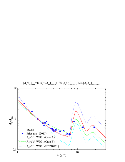
Figure 4: Comparison of the GC IR extinction of Fritz et al. (2011; blue squares) with the best fit model extinction (red solid line) obtained from the combination of three extinction curves of ${R_{\rm V}}=2.1$ (28%, dotted line), ${R_{\rm V}}=3.1$ (39%, dashed line), and ${R_{\rm V}}=5.5$ (33%, dot-dashed line). Also shown are the observed extinction toward the GC by Nishiyama et al. (2009; green triangles) and the best fit with our dust model (see $\S$3; red dotted line).

5 Summary

The ${\sim}\,$1–19$\,{\rm\mu m}$ IR extinction curve of the GC recently derived by Fritz et al. (2011) is fitted with a mixture of graphite and amorphous silicate dust. The model has difficulty in simultaneously reproducing the steep NIR extinction and the flat MIR extinction. The best-fit model estimates the total visual extinction toward the GC to be ${A_{\rm V}}\sim 38-42\,{\rm mag}$. In view that the starlight from the GC passes through different interstellar environments, the observed extinction curve toward the GC could be a combination of different extinction curves produced by grains with different size distributions characteristic of different environments: dust in diffuse regions (characterized by small ${R_{\rm V}}$ and steep near-IR extinction), and dust in dense regions (characterized by large ${R_{\rm V}}$ and flat UV extinction).

- [1] Cardelli, J. A., G. C. Clayton, and J. S. Mathis, The relationship between infrared, optical, and ultraviolet extinction, The Astrophysical Journal, 345, 245–256, 1989. (CCM)
- [2] Draine, B. T., Interstellar extinction in the infrared, Infrared Spectroscopy in Astronomy, 290, 93–98, 1989.
- [3] Draine, B. T., Interstellar Dust Grains, Annual Review of Astronomy and Astrophysics, 41, 241–289, 2003.
- [4] Draine, B. T. and H. M. Lee, Optical properties of interstellar graphite and silicate grains, The Astrophysical Journal, 285, 89–108, 1984.
- [5] Fitzpatrick, E. L. and D. Massa, An Analysis of the Shapes of Interstellar Extinction Curves. VI. The Near-IR Extinction Law, The Astrophysical Journal, 699, 1209–1222, 2009.
- [6] Flaherty, K. M., J. L. Pipher, S. T. Megeath, and et al., Infrared Extinction toward Nearby Star-forming Regions, The Astrophysical Journal, 663, 1069–1082, 2007.
- [7] Fritz, T. K., S. Gillessen, K. Dodds-Eden, D. Lutz, R. Genzel, W. Raab, T. Ott, O. Pfuhl, F. Eisenhauer, and F. Yusef-Zadeh, Line Derived Infrared Extinction toward the Galactic Center, The Astrophysical Journal, 737,73–2011.
- [8] Gao, J., B. W. Jiang, and A. Li, Toward understanding the 3.4 m and 9.7 m extinction feature variations from the local diffuse interstellar medium to the Galactic center, Earth, Planets, and Space, 62, 63–67, 2010.
- [9] Gao, J., B. W. Jiang, and A. Li, Mid-Infrared Extinction and its Variation with Galactic Longitude, The Astrophysical Journal, 707, 89–102, 2009.
- [10] Grevesse, N. and A. J. Sauval, Standard Solar Composition, Space Science Reviews, 85, 161-174, 1998.
- [11] Indebetouw, R., J. S. Mathis, B. L. Babler, and et al., The Wavelength Dependence of Interstellar Extinction from 1.25 to 8.0 m Using GLIMPSE Data, The Astrophysical Journal, 619, 931–938, 2005.
- [12] Jiang, B. W., J. Gao, A. Omont, and et al., Extinction at 7 m and 15 m from the ISOGAL survey, Astronomy and Astrophysics, 446, 551–560, 2006.
- [13] Jura, M., Origin of large interstellar grains toward Rho Ophiuchi, The Astrophysical Journal, 235, 63–65, 1980.
- [14] Larson, K. A., D. C. B. Whittet, and J. H. Hough, Interstellar Extinction, Polarization, and Grain Alignment in the High-Latitude Molecular Cloud toward HD 210121, The Astrophysical Journal, 472, 755–1996.
- [15] Li, A. and B. T. Draine, Infrared Emission from Interstellar Dust. II. The Diffuse Interstellar Medium, The Astrophysical Journal, 554, 778–802, 2001.
- [16] Li, A. and J. M. Greenberg, The dust extinction, polarization and emission in the high-latitude cloud toward HD 210121, Astronomy and Astrophysics, 339, 591–600, 1998.
- [17] Lutz, D., ISO observations of the Galactic Centre, The Universe as Seen by ISO, 427, 623, 1999.
- [18] McFadzean, A. D., D. C. B. Whittet, M. F. Bode, A. J. Adamson, and A. J. Longmore, Infrared studies of dust and gas towards the Galactic Centre – 3–5 spectroscopy, Monthly Notices of the Royal Astronomical Society, 241, 873–882, 1989.
- [19] Mathis, J. S., W. Rumpl, and K. H. Nordsieck, The size distribution of interstellar grains, The Astrophysical Journal,217, 425–433, 1977.
- [20] Nishiyama, S., T. Nagata, N. Kusakabe, and et al., Interstellar Extinction Law in the J, H, and Ks Bands toward the Galactic Center, The Astrophysical Journal, 638, 839–846, 2006.
- [21] Nishiyama, S., M. Tamura, H. Hatano, and et al., Interstellar Extinction Law Toward the Galactic Center III: J, H, KS Bands in the 2MASS and the MKO Systems, and 3.6, 4.5, 5.8, 8.0 m in the Spitzer/IRAC System, The Astrophysical Journal, 696, 1407–1417, 2009.
- [22] Nowak, M. A., J. Neilsen, S. B. Markoff, and et al., ChandraHETGS Observations of the Brightest Flare Seen from Sgr A, The Astrophysical Journal, 759, 95–104, 2012.
- [23] Rieke, G. H. and M. J. Lebofsky, The interstellar extinction law from 1 to 13 microns, The Astrophysical Journal, 288, 618–621, 1985. (RL85)
- [24] Rieke, G. H., M. J. Rieke, and A. E. Paul, Origin of the excitation of the galactic center, The Astrophysical Journal, 336, 752–761, 1989.
- [25] Weingartner, J. C. and B. T. Draine, Dust Grain-Size Distributions and Extinction in the Milky Way, Large Magellanic Cloud, and Small Magellanic Cloud, The Astrophysical Journal, 548, 296–309, 2001. (WD01)
- [26] Whittet, D. C. B., A. C. A. Boogert, P. A. Gerakines, W. A. Schutte, A. G. G. M. Tielens, T. deGraauw, T. Prusti, E. F. van Dishoeck, P. R. Wesselius, and C. M. Wright, Infrared Spectroscopy of Dust in the Diffuse ISM toward Cygnus OB2 No. 12, Astrophysical Journal, 490, 729–734, 1997.
- [27] Zasowski, G., S. R. Majewski, R. Indebetouw, and et al., Lifting the Dusty Veil with Near- and Mid-Infrared Photometry. II. A Large-Scale Study of the Galactic Infrared Extinction Law, The Astrophysical Journal, 707, 510–523, 2009.
- [28] Zubko, V., E. Dwek, and R. G. Arendt, Interstellar Dust Models Consistent with Extinction, Emission, and Abundance Constraints, The Astrophysical Journal Supplement Series, 152, 211–249, 2004.
- [29]