Matrix Product States for Quantum Many-Fermion Systems

Abstract

We describe a simple method to find the ground state energy without calculating the expectation value of the Hamiltonian in the time-evolving block decimation algorithm with tensor network states. For example, we consider quantum many-fermion systems with matrix product states, which are updated consistently in a way that accounts for fermion exchange effects. This method can be applied to a wide class of fermion systems. We test this method in spinless fermion system where the exact ground state energy is known. We analyze finite size effects to determine the ground state energy in the thermodynamic limit that is compared to the exact value.

1 Introduction

One of the main challenges in the field of quantum many-fermion systems is to invent an efficient computational method for finding the ground states. Up to now, various methods have been proposed such as exact diagonalization, quantum Monte Carlo, etc. However, exact diagonalization has limitations in the tractable system size, while quantum Monte Carlo is plagued by the fermion sign problem Troyer . A practical computational method is the diffusion Monte Carlo (DMC) Ceperley ; Chung1 , where a set of replicas is used to represent an approximate ground state. While the replicas are walking and branching, the number of replicas is controlled by changing the energy value.

As another accurate computational method without generating random numbers, the density-matrix renormalization group (DMRG) was invented by White White to simulate strongly correlated one-dimensional quantum lattice systems. The deeper understanding of the internal structure of the DMRG is allowed by the matrix product states (MPS) Vidal2 ; Vidal3 ; Schollwoeck ; Orus . The method of MPS have attracted much interests for decades in many different topics Ostlund ; Garcia ; Pirvu ; Silvi . Especially, using MPS, Vidal Vidal obtained a simple and fast algorithm for the simulation of quantum lattice spin systems in one-dimension. This clever approach is the local updates of tensors in the MPS by properly handling the Schmidt coefficients. The concept of local updates is further exploited for quantum lattice spin systems in two-dimension Jiang .

Tensor network states including MPS have been generalized to describe fermionic systems independently by several groups. The fermionic projected entangled-pair states Kraus ; Corboz ; Pizorn ; Corboz2 was introduced and multiscale entanglement renormalization ansatz Barthel ; Corboz3 ; Corboz4 ; Pineda ; Marti was generalized to fermionic lattice systems for the ground states of local Hamiltonians. These fermionic generalizations share some similarities, but they also differ in significant ways. Since a tensor network algorithm is one of variational methods, the difference between the generalizations can be recognized. It is remarkable that the infinite projected entangled-pair state for the ground state in the two-dimensional $t$-$J$ model exhibits stripes Corboz5 , which are in contrast to the uniform phase obtained by other calculations such as variational Monte Carlo and fixed-node Monte Carlo.

In this paper, getting back to basics for quantum many-fermion systems, we propose a slightly different algorithm from the previous approach. We use the concept of updating energy in DMC to simulate quantum many-fermion systems. We consider the time-evolving block decimation in imaginary time, including the energy parameter as in DMC. During the time evolution, we restrict the accessible states only to MPS. The time evolution of the MPS is essentially equivalent to the random process of walking and branching in DMC. The evolution of the MPS norm updates the value of ground state energy. For spinless fermion systems, we test this algorithm by comparing the result obtained by our method to the exact ground state energy. This approach could be a small but clear step to reach the solution of the two dimensional Hubbard model, which is one of the current challenging problems. For future works of tensor network states, we build a user-friendly library in the scheme of the previous computer code Chung2 ; Chung3 .

2 Algorithm

For a quantum system of $N$ sites and $M$ fermions, the typical dimension of the Hilbert space is determined by the number of combinations of selecting $M$ elements from $N$ distinct elements. Thus the dimension of the Hilbert space is an exponential function of $N$ and $M$. To overcome difficulties arising in the huge Hilbert space, one may use a small subspace of the Hilbert space: matrix product states (MPS) or projected entangled-pair states (PEPS) Verstraete . Here we focus on MPS to explain the algorithm for quantum many-fermion systems.

Representing MPS, we use $N$ three-index tensors $A^{\sigma_{i}}_{ab}$ and $N$ Schmidt coefficient vectors $\lambda_{a}^{i}$, where $i$ runs over all $N$ sites. To describe the feature of fermions, we impose that $\sigma_{i}=0$ or $1$ means vacancy or occupancy at the $i$-th site respectively. For the bond degree of freedom, the indices $a$ and $b$ run from $0$ to $D-1$. A typical state in the space of matrix product states is written as

$$|\Psi\rangle=\sum_{\sigma}\sum_{ab\cdots c}A^{\sigma_{0}}_{ab}\lambda^{0}_{b}\cdots A^{\sigma_{N-1}}_{ca}\lambda^{N-1}_{a}|\sigma_{0}\sigma_{1}\cdots\sigma_{N-1}\rangle,$$ (1)

where index-contraction is done as shown in Fig. 1. It is important to notice one-to-one correspondence between a state of the spin-like chain represented by $\sigma_{i}$ and a state of the Fock space written in terms of creation operators $c^{\dagger}_{i}$ such as

$$|\sigma_{0}\sigma_{1}\cdots\sigma_{N-1}\rangle=c^{\dagger}_{i_{0}}c^{\dagger}_{i_{1}}\cdots c^{\dagger}_{i_{M-1}}|0\rangle,$$ (2)

where $\sigma_{i}=1$ if $i\in\{i_{0},i_{1},\cdots,i_{M-1}\}$ or $0$ otherwise so that $\sigma_{0}+\sigma_{1}+\cdots+\sigma_{N-1}=M$.

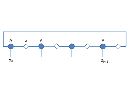
Figure 1: Diagrammatic representation of a coefficient in front of an orthonormal basis in $|\Psi\rangle$. Closed circles and open diamonds represent tensors $A$ and the Schmidt coefficients $\lambda$, respectively. For a periodic boundary condition, site $N-1$ connects back to site $0$. This connection corresponds to the trace operation.

For a given Hamiltonian $H$, introducing an energy shift $E$ and the inverse of energy $t$, we consider a formal solution of the imaginary time Schrödinger equation:

$$|\Psi(t)\rangle=\exp\{-(H-E)t\}|\Psi(0)\rangle.$$ (3)

As $t$ goes to infinity, the state $|\Psi(t)\rangle$ becomes the ground state for properly chosen $E$. This is the basic idea of DMC. The convergence of $E$ is a necessary condition for the ground state to be stable.

Since we simulate an evolution in the space of MPS, $|\Psi(t)\rangle$ does not keep a constant number of fermions, while the Hamiltonian $H$ does not change the number of fermions. To overcome this problem, we can introduce the chemical potential $\mu$ and replace $H$ by $H+\mu\sum_{i}c^{\dagger}_{i}c_{i}$. However, as far as we are interested in the true ground state, we do not need $\mu$ because the eventual ground state $|\Psi(\infty)\rangle$ will sharply peak at some $M$ without $\mu$.

We assume that $H$ is defined by the sum of local operators such as

$$H=\sum_{\alpha}h_{\alpha}.$$ (4)

For a given small time step $\tau$, we introduce the Suzuki-Trotter decomposition as

$$\exp\{-(H-E)t\}\approx\prod^{t/\tau}\prod_{\alpha}\exp\{(e-h_{\alpha})\tau\},$$ (5)

where $e=E/(\sum_{\alpha}1)$ and we should take care of the order of $\alpha$ for error minimization, for example, $\prod_{\alpha}=\prod_{\alpha=\text{odd}}\prod_{\alpha=\text{even}}$. We act the operator $\prod_{\alpha}\exp\{(e-h_{\alpha})\tau\}$ consecutively on the state $|\Psi_{n}\rangle$ to generate $|\Psi_{n+1}\rangle$, $|\Psi_{n+2}\rangle$, and so on. The key point is that each output state $\exp\{(e-h_{\alpha})\tau\}|\text{MPS}\rangle$, which is outside of the space of MPS, is approximated into a MPS. As $t$ goes to infinity, we obtain the approximate ground state in the form of MPS.

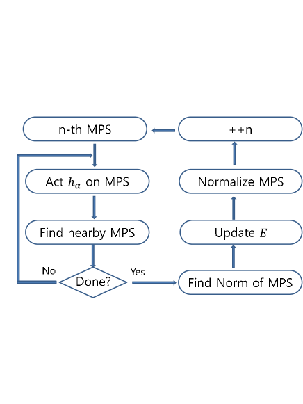
Figure 2: Flow chart of the algorithm.

In our algorithm, we start with a normalized MPS $|\Psi_{n}\rangle$. After we act $\prod_{\alpha}\exp\{(e-h_{\alpha})\tau\}$ on $|\Psi_{n}\rangle$ and find an output MPS $|\bar{\Psi}_{n+1}\rangle$, we calculate the norm of $|\bar{\Psi}_{n+1}\rangle$. If the norm is larger (smaller) than 1, we adjust $e$ to become smaller (larger) such as $e_{n+1}=e_{n}+\xi(1-\langle\bar{\Psi}_{n+1}|\bar{\Psi}_{n+1}\rangle)$ with a small positive parameter $\xi$. We replace $|\bar{\Psi}_{n+1}\rangle$ by the normalized one, and call it $|\Psi_{n+1}\rangle$ for the next iteration. Our algorithm is summarized in Fig. 2.

3 One-Body Interaction

The main step in our algorithm is to find the approximate MPS after we act $\exp\{(e-h_{\alpha})\tau\}$ on the previous MPS. Usually $h_{\alpha}$ is decomposed into a diagonal Hamiltonian $h^{d}_{\alpha}$ and an off-diagonal Hamiltonian $h^{o}_{\alpha}$ such as

$$\exp\{(e-h_{\alpha})\tau\}\approx\exp\{(e-h^{d}_{\alpha})\tau\}\exp(-h^{o}_{\alpha}\tau).$$ (6)

The diagonal Hamiltonian expands or contracts all basis vectors without changing direction, while the off-diagonal Hamiltonian changes both direction and length of bases. For instance, in the Fock space, the Coulomb repulsion of $Vc^{\dagger}_{i}c_{i}c^{\dagger}_{j}c_{j}$ is a diagonal Hamiltonian for the basis of occupation number representation. For an off-diagonal Hamiltonian, there are two cases in physical interests: one-body interaction,

$$-h^{o}_{\alpha}\tau=d\exp(i\theta)c^{\dagger}_{i}c_{j}+d\exp(-i\theta)c^{\dagger}_{j}c_{i},$$ (7)

and two-body interaction,

$$-\tilde{h}^{o}_{\alpha}\tau=d\exp(i\theta)c^{\dagger}_{i}c^{\dagger}_{j}c_{k}c_{l}+d\exp(-i\theta)c^{\dagger}_{l}c^{\dagger}_{k}c_{j}c_{i}.$$ (8)

For simplicity, we here consider the procedure for one-body interaction only. We will extend our method to two-body interaction in the future.

With the one-body interaction $-h^{o}_{\alpha}\tau$ of Eq. (7), we act $\exp(-h^{o}_{\alpha}\tau)$ on a basis vector $|\sigma_{0}\cdots\sigma_{i}\cdots\sigma_{j}\cdots\sigma_{N-1}\rangle$. A simple calculation allows us to find the important result written in four cases in terms of $\sigma_{i}=0$ or $1$ and $\sigma_{j}=0$ or $1$:

$$\left\{\begin{array}[]{l}\exp(-h^{o}_{\alpha}\tau)|\cdots 0\cdots 0\cdots\rangle=|\cdots 0\cdots 0\cdots\rangle\\ \exp(-h^{o}_{\alpha}\tau)|\cdots 0\cdots 1\cdots\rangle=\cosh d|\cdots 0\cdots 1\cdots\rangle\\ ~{}~{}+\sinh d\exp(i\theta)(-1)^{\sigma_{i+1}+\cdots+\sigma_{j-1}}|\cdots 1\cdots 0\cdots\rangle\\ \exp(-h^{o}_{\alpha}\tau)|\cdots 1\cdots 0\cdots\rangle=\cosh d|\cdots 1\cdots 0\cdots\rangle\\ ~{}~{}+\sinh d\exp(-i\theta)(-1)^{\sigma_{i+1}+\cdots+\sigma_{j-1}}|\cdots 0\cdots 1\cdots\rangle\\ \exp(-h^{o}_{\alpha}\tau)|\cdots 1\cdots 1\cdots\rangle=|\cdots 1\cdots 1\cdots\rangle\end{array}\right.$$

It is innovative that the sign of $(-1)^{\sigma_{i+1}+\cdots+\sigma_{j-1}}$ is based on the fermion exchange. The above equations are used to update the MPS represented in new tensors $\tilde{A}$ and new weights $\tilde{\lambda}$. Since $\exp(-h^{o}_{\alpha}\tau)$ locally changes $|\Psi\rangle$, the outside tensors and weights remain unchanged such as $\tilde{A}^{\sigma_{k}}=A^{\sigma_{k}}$ for $k<i$ or $k>j$ and $\tilde{\lambda}^{k}=\lambda^{k}$ for $k<i$ or $k>j-1$. We should determine $\tilde{A}^{\sigma_{l}}$ for $i\leq l\leq j$ and $\tilde{\lambda}^{l}$ for $i\leq l\leq j-1$ by using the method proposed by Vidal Vidal . We first define a $(2+j-i+1)$-index tensor $M^{\sigma_{i}\cdots\sigma_{j}}_{ab}$ such as

$$M^{\sigma_{i}\sigma_{i+1}\cdots\sigma_{j-1}\sigma_{j}}_{ab}\equiv\sum_{cd\cdots fg}\lambda_{a}^{i-1}A^{\sigma_{i}}_{ac}\lambda_{c}^{i}A^{\sigma_{i+1}}_{cd}\lambda_{d}^{i+1}$$

$$\cdots\lambda_{f}^{j-2}A^{\sigma_{j-1}}_{fg}\lambda_{g}^{j-1}A^{\sigma_{j}}_{gb}\lambda_{b}^{j}.$$ (9)

Then we find a single $(2+j-i+1)$-index tensor $\Theta^{\sigma_{i}\cdots\sigma_{j}}_{ab}$ which will be written in the matrix product form:

$$\left\{\begin{array}[]{l}\Theta^{0\sigma_{i+1}\cdots\sigma_{j-1}0}_{ab}=M^{0\sigma_{i+1}\cdots\sigma_{j-1}0}_{ab}\\ \Theta^{0\sigma_{i+1}\cdots\sigma_{j-1}1}_{ab}=M^{0\sigma_{i+1}\cdots\sigma_{j-1}1}_{ab}\cosh d\\ ~{}~{}+M^{1\sigma_{i+1}\cdots\sigma_{j-1}0}_{ab}\sinh d\exp(-i\theta)(-1)^{\sigma_{i+1}+\cdots+\sigma_{j-1}}\\ \Theta^{1\sigma_{i+1}\cdots\sigma_{j-1}0}_{ab}=M^{1\sigma_{i+1}\cdots\sigma_{j-1}0}_{ab}\cosh d\\ ~{}~{}+M^{0\sigma_{i+1}\cdots\sigma_{j-1}1}_{ab}\sinh d\exp(i\theta)(-1)^{\sigma_{i+1}+\cdots+\sigma_{j-1}}\\ \Theta^{1\sigma_{i+1}\cdots\sigma_{j-1}1}_{ab}=M^{1\sigma_{i+1}\cdots\sigma_{j-1}1}_{ab}\end{array}\right.$$

The new tensors are determined by singular value decomposition (SVD) of $\Theta$ such as

$$\Theta^{\sigma_{i}\cdots\sigma_{j}}_{ab}\approx\sum_{cd\cdots fg}\bar{A}^{\sigma_{i}}_{ac}\tilde{\lambda}_{c}^{i}\tilde{A}^{\sigma_{i+1}}_{cd}\tilde{\lambda}_{d}^{i+1}\cdots\tilde{A}^{\sigma_{j-1}}_{fg}\tilde{\lambda}_{g}^{j-1}\bar{A}^{\sigma_{j}}_{gb}.$$ (10)

To finish updating, we attach the inverse of the Schmidt coefficients $\tilde{\lambda}$ to the first tensor $\bar{A}^{\sigma_{i}}$ and the last tensor $\bar{A}^{\sigma_{j}}$ in Eq. (10) such as

$$\tilde{A}^{\sigma_{i}}_{ac}=\bar{A}^{\sigma_{i}}_{ac}/\tilde{\lambda}^{i-1}_{a},~{}~{}~{}~{}\tilde{A}^{\sigma_{j}}_{gb}=\bar{A}^{\sigma_{j}}_{gb}/\tilde{\lambda}^{j}_{b}.$$ (11)

Compared to the vigorous calculation in dealing with the off-diagonal Hamiltonian, the diagonal Hamiltonian is simple and straightforward to handle. Acting $\exp\{(e-h^{d}_{\alpha})\tau\}$ on the MPS, we can easily find the relation between old tensors $A$ and new tensors $\tilde{A}$. In order to update the MPS, we take the same procedure described in the above: find $\Theta$, do SVD, and attach $\lambda$.

4 Spinless Fermion System

We have tested our method by calculating the ground state energy and the wave function for spinless fermion system Rozhkov , where the exact ground state energy is known. The corresponding Hamiltonian is written as

$$H=\sum_{i=0}^{N-1}\{-u(c_{i}^{\dagger}c_{i+1}+c_{i+1}^{\dagger}c_{i})+v(n_{i}-\frac{1}{2})(n_{i+1}-\frac{1}{2})\},$$ (12)

where $n_{i}=c_{i}^{\dagger}c_{i}$ and the periodic boundary condition is imposed by $c_{N}\equiv c_{0}$.

In this model, the real value $d$ in Eq. (7) is given by the hopping parameter $u$ times $\tau$, and that the phase $\theta$ in Eq. (7) is simply equal to zero. When we act $\exp(-h^{o}_{\alpha}\tau)$ on the MPS, the four-index tensor $M^{\sigma_{i}\sigma_{i+1}}_{ab}$ in Eq. (9) is involved because the model has only the nearest neighbor interaction. We follow the procedure up to Eq. (11) to update the tensors $A^{\sigma_{i}}_{ab}$ and the weights $\lambda^{i}_{a}$.

Considering the evolution by $\exp\{(e-h^{d}_{\alpha})\tau\}$ in this model with $e=E/N$, we obtain the single four-index tensor such as

$$\Theta^{\sigma_{i}\sigma_{i+1}}_{ab}=\sum_{c}\lambda_{a}^{i-1}A^{\sigma_{i}}_{ac}\lambda_{c}^{i}A^{\sigma_{i+1}}_{cb}\lambda_{b}^{i+1}$$

$$\times\exp\{[e-v(\sigma_{i}-\frac{1}{2})(\sigma_{i+1}-\frac{1}{2})]\tau\}.$$ (13)

Keeping $D$ largest weights $\tilde{\lambda}^{i}_{c}$ among $2D$ values in SVD of $\Theta^{\sigma_{i}\sigma_{i+1}}_{ab}$, we obtain the approximate tensor as shown in Eq. (10). We attach the inverse of the Schmidt coefficients to update the tensors $A$ as shown in Eq. (11).

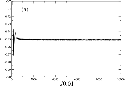
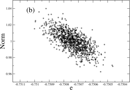
Figure 3: (a) The energy value $e$ as a function of the time $t/\tau$ for $N=400$ and $D=10$. We let the initial value of $e$ be zero. We find that the MPS is not changed much after $t=10$. It seems that the MPS is stable forever. (b) The scatter diagram for the sequence of data $(e_{n},\text{Norm}_{n})$ from $n=9001$ to $n=10000$. The thousand points in the scatter diagram shows negative association as expected.

Table 1: Numerical results on the average $\langle e\rangle$, the standard deviation $\delta$ for ground state energy, and the difference between $\langle e\rangle$ and the fitted value $\tilde{e}$ in spinless fermion system of $u=1$ and $v=1$.

$\tau$	$N$	$D$	$\langle e\rangle\pm\delta$	$\langle e\rangle-\tilde{e}$
0.02	100	4	$-0.75055\pm 0.00023$	$-0.00011$
		5	$-0.75190\pm 0.00025$	$0.00018$
		6	$-0.75272\pm 0.00021$	$0.00008$
0.02	200	4	$-0.74856\pm 0.00019$	$0.00009$
		5	$-0.75039\pm 0.00022$	$-0.00011$
		6	$-0.75114\pm 0.00020$	$-0.00013$
0.01	100	4	$-0.75046\pm 0.00014$	$-0.00020$
		5	$-0.75175\pm 0.00012$	$0.00014$
		6	$-0.75262\pm 0.00011$	$-0.00001$
		10	$-0.75325\pm 0.00009$	$0.00014$
0.01	200	4	$-0.74850\pm 0.00011$	$-0.00003$
		5	$-0.75031\pm 0.00011$	$-0.00021$
		6	$-0.75108\pm 0.00010$	$-0.00026$
		10	$-0.75165\pm 0.00009$	$-0.00005$
0.01	400	4	$-0.74742\pm 0.00012$	$0.00015$
		5	$-0.74886\pm 0.00011$	$0.00035$
		6	$-0.74993\pm 0.00010$	$-0.00000$
		10	$-0.75074\pm 0.00008$	$-0.00004$

The simulations were performed for the case of $u=1$ and $v=1$ by fixing $\xi=0.01$ in the energy update of $e_{n+1}=e_{n}+\xi(1-\text{Norm}_{n+1})$. For given $N$ and $D$ with various $\tau$, the simulation study shows that the energy $e$ is converging. Fig. 3(a) shows the convergence of $e$ for $\tau=0.01$, $N=400$ and $D=10$. We determine the ground state energy by taking the average $\langle e\rangle$ after annealing for a long time ($t=90$). Truncation of original states caused by approximation makes the MPS look like random as shown in Fig. 3(b). The numerical results of the average $\langle e\rangle$ as the estimates of the ground state energy and the standard deviation $\delta$ are summarized in Table 1, where we notice finite size effects. To reduce the finite size effects, we may need larger values of $N$ and $D$, and a smaller value of $\tau$ as well as a higher-order Suzuki-Trotter decomposition than that of Eq. (5). Using the results in Table 1, we analyze the finite size effects with least squares fitting, and determine the fitting parameters in $\tilde{e}(\tau,N,D)$ for the ground state energy as

$$\tilde{e}(\tau,N,D) = -0.74996(7)-0.608(9)\tau^{2}$$ (14)

$$- 0.358(3)\frac{1}{N}+0.214(4)\frac{1}{D^{3}}.$$

The computation time is roughly proportional to $ND^{\alpha}$ with $\alpha$ ranging from $6$ to $7$.

5 Conclusion

Summing up, we have presented an improved time-evolving block decimation including the energy parameter to obtain the ground state energy and wave function for quantum many-fermion systems. If a system has translational symmetry, it is possible to parallelize local updates Vidal . In other words, a single (or a few) $A$ and $\lambda$ are enough to describe our process. However, we have not presented this special case here because we are focusing on a general algorithm, which is applicable to all cases. We will extend our method to PEPS for two-dimensional quantum many-fermion systems. The higher-order SVD deLathauwer ; Levin ; Xie may be useful when we calculate the norm of PEPS. Furthermore, switching from imaginary time to real time in Eq. (3) and changing the Hamiltonian slightly, we may simulate the time evolution from the ground state in order to explain experimental data of quenching.

References

• (1) M. Troyer, U.-J. Wiese, Phys. Rev. Lett. 94, 170201 (2005)
• (2) D. Ceperley, B. Alder, Science 231, 555 (1986)
• (3) M.-H. Chung, D. P. Landau, Phys. Rev. B 85, 115115 (2012)
• (4) S. R. White, Phys. Rev. Lett. 69, 2863 (1992)
• (5) G. Vidal, Phys. Rev. Lett. 91, 147902 (2003)
• (6) G. Vidal, Phys. Rev. Lett. 93, 040502 (2004)
• (7) U. SchollwΓΆck, Ann. Phys. 326, 96 (2011)
• (8) R. OrΓΊs, Phys. Rev. B 85, 205117 (2012)
• (9) S. Γ–stlund, S. Rommer, Phys. Rev. Lett. 75, 3537 (1995)
• (10) J. J. GarcΓ­a-Ripoll, New J. Phys. 8, 305 (2006)
• (11) B. Pivru, G. Vidal, F. Verstraete, L. Tagliacozzo, Phys. Rev. B 86, 075117 (2012)
• (12) P. Silvi, D. Rossini, R. Fazio, G. E. Santoro, V. Giovannetti, Int. J. Mod. Phys. B 27, 1345029 (2013)
• (13) G. Vidal, Phys. Rev. Lett. 98, 070201 (2007)
• (14) H. C. Jiang, Z. Y. Weng, T. Xiang, Phys. Rev. Lett. 101, 090603 (2008)
• (15) C. V. Kraus, N. Schuch, F. Verstraete, J. I. Cirac, Phys. Rev. A 81, 052338 (2010)
• (16) P. Corboz, R. OrΓΊs, B. Bauer, G. Vidal, Phys. Rev. B 81, 165104 (2010)
• (17) I. PiΕΎorn, F. Verstraete, Phys. Rev. B 81, 245110 (2010)
• (18) P. Corboz, J. Jordan, G. Vidal, Phys. Rev. B 82, 245119 (2010)
• (19) T. Barthel, C. Pineda, J. Eisert, Phys. Rev. A 80, 042333 (2009)
• (20) P. Corboz G. Vidal, Phys. Rev. B 80, 165129 (2009)
• (21) P. Corboz, G. Evenbly, F. Verstraete, G. Vidal, Phys. Rev. A 81, 010303 (2010)
• (22) C. Pineda, T. Barthel, J. Eisert, Phys. Rev. A 81, 050303 (2010)
• (23) K. H. Marti, B. Bauer, M. Reiher, M. Troyer, F. Verstraete, New J. Phys. 12, 103008 (2010)
• (24) P. Corboz, S. R. White, G. Vidal, M. Troyer, Phys. Rev. B 84, 041108 (2011)
• (25) M.-H. Chung, Int. J. Mod. Phys. C 15, 185 (2004)
• (26) M.-H. Chung, Sci. Comput. Program. 71, 242 (2008)
• (27) D. PΓ©rez-GarcΓ­a, F. Verstraete, M. M. Wolf, J. I Cirac, Quant. Inf. Comp. 8, 0650 (2008)
• (28) A. V. Rozhkov, Phys. Rev. B 85, 045106 (2012)
• (29) L. de Lathauwer, B. de Moor, J. Vandewalle, SIAM J. Matrix Anal. Appl. 21, 1253 (2000)
• (30) M. Levin, C. P. Nave, Phys. Rev. Lett. 99, 120601 (2007)
• (31) Z. Y. Xie, J. Chen, M. P. Qin, J. W. Zhu, L. P. Yang, T. Xiang, Phys. Rev. B 86, 045139 (2012)