Multi-Color Transit Photometry of GJ 1214b through BJHK_s-Bands
and a Long-Term Monitoring of the Stellar Variability of GJ 1214

Abstract

We present 5 new transit light curves of GJ 1214b taken in $BJHK_{\rm s}$-bands. Two transits were observed in $B$-band using the Suprime-Cam and the FOCAS instruments onboard the Subaru 8.2m telescope, and one transit was done in $JHK_{\rm s}$-bands simultaneously with the SIRIUS camera on the IRSF 1.4m telescope. MCMC analyses show that the planet-to-star radius ratios are, $R_{\rm p}/R_{\rm s}=0.11651\pm 0.00065$ ($B$-band, Subaru/Suprime-Cam), $R_{\rm p}/R_{\rm s}=0.11601\pm 0.00117$ ($B$-band, Subaru/FOCAS), $R_{\rm p}/R_{\rm s}=0.11654\pm 0.00080$ ($J$-band, IRSF/SIRIUS), $R_{\rm p}/R_{\rm s}=0.11550^{+0.00142}_{-0.00153}$ ($H$-band, IRSF/SIRIUS), and $R_{\rm p}/R_{\rm s}=0.11547\pm 0.00127$ ($K_{\rm s}$-band, IRSF/SIRIUS). The Subaru Suprime-Cam transit photometry shows a possible spot-crossing feature. Comparisons of the new transit depths and those from previous studies with the theoretical models by Howe & Burrows (2012) suggest that the high molecular weight atmosphere (e.g., 1% H₂O + 99% N₂) models are most likely, however, the low molecular weight (hydrogen dominated) atmospheres with extensive clouds are still not excluded. We also report a long-term monitoring of the stellar brightness variability of GJ 1214 observed with the MITSuME 50cm telescope in $g^{\prime}$-, $R_{\mathrm{c}}$-, and $I_{\mathrm{c}}$-bands simultaneously. The monitoring was conducted for 32 nights spanning 78 nights in 2012, and we find a periodic brightness variation with a period of $P_{\rm s}=44.3\pm 1.2$ days and semi-amplitudes of 2.1%$\pm$0.4% in $g^{\prime}$-band, 0.56%$\pm$0.08% in $R_{\mathrm{c}}$-band, and 0.32%$\pm$0.04% in $I_{\mathrm{c}}$-band.

1 Introduction

Super-earths are an emerging population of extrasolar planets whose masses and radii lie between those of the Earth and the Uranus/Neptune. The nature of super-Earths, such as internal structure and atmospheric compositions, remains almost unknown since there is no super-Earth in our Solar System. Transiting super-Earths are thus invaluable targets for observations to learn the nature of super-Earths in details.

GJ 1214b discovered by Charbonneau et al. (2009) is the first-ever transiting super-Earth around an M dwarf which enables us to study its atmosphere through so-called transmission spectroscopy, thanks to the small host star’s size ($\sim 0.2R_{\odot}$). For the purpose, a number of observers have measured transit depths of GJ 1214b in various wavelength regions (e.g., Bean et al. 2010, 2011; Croll et al. 2011; Désert et al. 2011a; Carter et al. 2011; Berta et al. 2011, 2012; de Mooij et al. 2012; Narita et al. 2013; Fraine et al. 2013; Teske et al. 2013), and have narrowed down possible atmospheric models proposed by theorists (e.g., Miller-Ricci & Fortney 2010; Howe & Burrows 2012; Benneke & Seager 2012).

Among recent publications, Howe & Burrows (2012) reported various atmospheric models and compared them with the previous observations. They concluded that a hydrogen-rich atmosphere with a haze of small ($\sim 0.1\mu$m) particles is the most likely model for GJ 1214b, however, they also noted that this is only valid if the Rayleigh scattering feature (a rise of transit depths in short optical wavelength) claimed by de Mooij et al. (2012) in the optical $g$-band is true. Howe & Burrows (2012) also reported that if the short-wavelength result is inaccurate, then alternative likely models are (1) an N₂ and water dominated atmosphere, (2) a solar-abundance (hydrogen dominated) atmosphere, with thick clouds at or above the 1 mbar level, or (3) a solar-abundance atmosphere with a haze of $\geq 1\mu$m particles. In those alternative cases, however, deeper $K_{\rm s}$-band transits claimed by Croll et al. (2011) and de Mooij et al. (2012) are incompatible with the models. Thus the discussions of likely atmospheric models are largely depend on the reliability of the results by Croll et al. (2011) and de Mooij et al. (2012).

Motivated by this fact, we previously tried simultaneous $JHK_{\rm s}$-transit photometry of GJ 1214b using the SIRIUS camera on the IRSF 1.4m telescope in 2011 (Narita et al., 2013). Consequently, we did not find a deeper transit in $K_{\rm s}$-band; namely our result was inconsistent with the results by Croll et al. (2011) and de Mooij et al. (2012), and instead support a shallower transit reported by Bean et al. (2011). This result has raised the possibility of the alternative models by Howe & Burrows (2012).

Moreover, Teske et al. (2013) recently presented new $g^{\prime}$- and $V$-band transits, which was shallower than the $g$-band transit by de Mooij et al. (2012). Their results were still consistent with de Mooij et al. (2012), but also consistent with no Rayleigh scattering (water-dominated atmosphere) model due to large uncertainty in $R_{\rm p}/R_{\rm s}$. Although the $g$-band result by de Mooij et al. (2012) could not be explained without the Rayleigh scattering, the new results by Teske et al. (2013) raised fundamental questions whether or not the Rayleigh scattering feature is actually present. Thus the argument of the presence of the Rayleigh scattering in the atmosphere of GJ 1214b is still unsolved.

More recently, Fraine et al. (2013) presented new Spitzer photometry and also conducted comparisons of various atmospheric models with all of the previous observations. They found that the best-fit model was one of the alternative models in Howe & Burrows (2012), which contains 1% H₂O + 99% N₂ with a thick tholin haze of $0.1\mu$m particles. They also mentioned that a pure water model and a flat line (no atmosphere) model are still acceptable at the time of their publication.

Based on the previous discussions, we consider that remaining important keys to distinguish atmosphere models of GJ 1214b are (1) confirmation of a rise of transit depths in optical blue region due to the Rayleigh scattering, and (2) further confirmation of $K_{\rm s}$-band transit depths compared to $J$-band ones. To address the above problems, we conducted $B$-band (bluer than $g$- and $g^{\prime}$-band) transit observations with the Subaru 8.2m telescope to confirm or constrain the Rayleigh scattering feature, and also conducted follow-up transit observations in $JHK_{\rm s}$-bands with the IRSF 1.4m telescope in South Africa to check the transit depths in those bands once again.

Meanwhile it is also important to learn and estimate the systematic effects due to the stellar variability for implications of transit depths. Previously Berta et al. (2011) reported $\sim 3.5$ mmag stellar brightness variability in MEarth band (similar to $i+z$ band) with a period of $\sim 53$ days and $\sim 7$ mmag variability in $V$ band with a period of $\sim 41$ days. However, no independent confirmation of the stellar variability was reported. For this reason, we additionally monitored long-term stellar brightness variability with the MITSuME 50cm telescope at Okayama Astrophysical Observatory (OAO) in $g^{\prime}$-, $R_{c}$-, and $I_{c}$-bands spanning 78 nights to examine any systematic effect due to the stellar variability of GJ 1214. All the listed observations were conducted in 2012.

In this paper, we report results of the above new observations and present discussions on atmosphere models of GJ 1214b. The rest of the paper is organized as follows, We summarize our observations and methods of data reductions in Section 2. We describe analyses of transit light curves and stellar variability in Section 3. We present results of our analyses and discuss implications of the results in Section 4. Finally, we summarize this paper in Section 5.

2 Observations and Data Reductions

2.1 Subaru 8.2m Telescope

We observed two transits of GJ 1214b with the Subaru 8.2m telescope on the top of Mauna Kea, Hawaii, USA. We used the Subaru Prime Focus Camera (Suprime-Cam: Miyazaki et al. 2002) on 2012 August 12 UT and the Faint Object Camera and Spectrograph (FOCAS: Kashikawa et al. 2002) on 2012 October 8 UT. Both transits were observed through the Johnson-Cousins $B$-band filter ($0.440\mu{\rm m}\pm 0.054\mu{\rm m}$).

The Suprime-Cam equips a mosaic of ten fully-depleted-type 2K$\times$4K CCDs manufactured by Hamamatsu Photonics K.K., which covers a 34’$\times$27’ field of view (FOV) in total with a pixel scale of 0.20” pixel^-1 (each CCD has a FOV of 6.8’ $\times$ 13.6’). GJ 1214 was observed with the Suprime-Cam during 06:20–10:10 of 2012 August 12 UT. The condition was photometric through the observations. The exposure time was set to 40 s and the dead time (including the CCD readout time of 18 s and other setup times) was about 29 s (duty cycle of 58%). We took 185 frames in total with the Suprime-Cam. GJ 1214 was located in the 5th CCD chip, named “satsuki.” We defocused the telescope so that stars have doughnut-like point spread function (PSF) to achieve higher photometric precision. The typical size of the PSF was $\sim 15$ pixels ($\sim$3”) in radius. Primary data reduction, including bias subtraction and flat fielding, and aperture photometry was carried out with a customized pipeline by Fukui et al. (2011), with a constant aperture-size mode where a same aperture size is applied for all images.

The FOCAS is installed at the Cassegrain focus of the Subaru telescope. The camera has a circular FOV of 6’ in diameter, covered by two fully-depleted-type 2K$\times$4K CCDs by Hamamatsu Photonics K.K. Each CCD has four readout channels and each channel has 512$\times$4176 active pixels. The pixel scale is 0.104” pixel^-1. Note that the CCDs of the Suprime-Cam and the FOCAS are different. We observed GJ 1214 with the FOCAS during 04:46–07:08 of 2012 October 8 UT. The weather on that night was clear, but the observation started just after dusk and the first-half of the transit was occurred during twilight. The exposure time was 40 s and the dead time was about 22 s (duty cycle of 65%). We obtained 130 frames in total with the FOCAS. We again defocused the telescope and the typical size of the PSF was $\sim 17$ pixels ($\sim$1.8”) in radius. Primary reduction for bias subtraction using overscan region was processed with a dedicated tool named FOCASRED. Subsequent procedures, such as flat fielding and aperture photometry, were conducted with the same customized pipeline (Fukui et al., 2011) as the case for the Suprime-Cam.

2.2 IRSF 1.4m Telescope

We observed a full transit of GJ 1214b with the Infrared Survey Facility (IRSF) 1.4m telescope located in Sutherland, South Africa. The transit was observed during 19:26–21:40 of 2012 June 14 UT. We used Simultaneous Infrared Imager for Unbiased Survey (SIRIUS: Nagayama et al. 2003) camera for the observation, which is the same instrument we used in Narita et al. (2013). The SIRIUS camera is equipped with two dichroic mirrors and three 1K$\times$1K HgCdTe detectors, which can observe $J$- ($1.250\mu{\rm m}\pm 0.085\mu{\rm m}$), $H$- ($1.63\mu{\rm m}\pm 0.15\mu{\rm m}$), $K_{\rm s}$- ($2.14\mu{\rm m}\pm 0.16\mu{\rm m}$) bands simultaneously. The FOV of the SIRIUS camera is a square of 7.7’ on a side and a pixel scale is 0.45” pixel^-1. The exposure times were set to 40 s and the dead time of the SIRIUS is about 8 s (duty cycle of 83%). We obtained 163 frames on the night.

During observations, we used a position locking software introduced in Narita et al. (2013). Thanks to this software, positions of GJ 1214’s centroid on the three detectors were kept within an rms of about 2 pixels in both X and Y directions. We note that stellar images were widely defocused so that the PSF was spread to $\sim$16 pixels ($\sim$7”) in radius.

Data reduction for the IRSF data is carried out with a dedicated pipeline for the SIRIUS, including a correction for non-linearity, dark subtraction, and flat fielding. The non-linearity correction enables us to work up to $\sim$25000 ADU with $\leq$1% linearity, which is sufficient for the current observations (Narita et al., 2013). Subsequent aperture photometry was done with the pipeline by Fukui et al. (2011).

2.3 MITSuME 50cm Telescope

We monitored brightness of GJ 1214 for 32 nights spanning from 2012 August 15 to 2012 November 1 (spanning 78 nights in total) with the MITSuME 50cm telescope located in Okayama Astrophysical Observatory, Okayama, Japan. The purpose of those observations is not for planetary transits but for stellar variability monitoring. The MITSuME telescope is equipped with three 1K$\times$1K CCD cameras, which can obtain $g^{\prime}$-, $R_{\mathrm{c}}$-, and $I_{\mathrm{c}}$-band images simultaneously (Kotani et al., 2005; Yanagisawa et al., 2010). The each CCD has the pixel scale of 1^′′.5 pixel^-1 and the FOV is 26${}^{\prime}\times$ 26^′. We obtained about 10–80 frames per clear night. The exposure time was 60 s and the dead time was 3 s for all bands. We slightly defocused the MITSuME telescope so that the target did not saturate in $I_{\mathrm{c}}$-band. The PSF extends about 2–4 pixels or 3^′′–6^′′ in radius. We note that the contamination from objects surrounding the target and reference stars are negligible, because there is no bright object around the stars based on the 2MASS All-Sky Catalog of Point Sources (Cutri et al., 2003), and we have checked that the PSFs of the stars do not show significant contamination. Data reduction and aperture photometry for the MITSuME data are carried out with the pipeline by Fukui et al. (2011) as with the case for the Suprime-Cam.

3 Analyses

3.1 Transit Light Curves

First, we create dozens of trial light curves using different aperture sizes ($\Delta r$) and combinations of comparison stars for each observation. For the comparison stars, we use such stars that are not saturated, nor variable stars, and in the same CCD chip with GJ 1214. On this occasion we convert the time system, which is recorded in the FITS headers in units of Modified Julian Day (MJD) based on Coordinated Universal Time (UTC), to Barycentric Julian Day (BJD) based on Barycentric Dynamical Time (TDB) using the algorithm by Eastman et al. (2010). Note that the time for each datum is assigned as the mid-time of each exposure. We find all the trial light curves $F_{\rm obs}$ exhibit trends at out-of-transit (OOT) phase. The trends could be caused by slow variability in the brightness of GJ1214 itself or comparison stars, changing airmass, position changes of the stars on the detectors, or high sky background, and so on. We then check the all trial light curves by eye and eliminate obviously poor-quality ones.

Second, in order to select the most appropriate light curve for each observation and its baseline correction model for OOT phase, we adopt the Bayesian Information Criteria (BIC: Schwarz 1978) for our analyses. The BIC value is given by $\mathrm{BIC}\equiv\chi^{2}+k\ln N$, where $k$ is the number of free parameters, and $N$ is the number of data points. We fit the trial light curves with an analytic transit light curve model and various baseline models simultaneously.

For the transit light curve model, we employ a customized code (Narita et al., 2007) that use the analytic formula by Ohta et al. (2009), which is equivalent with Mandel & Agol (2002) when using the quadratic limb-darkening law. The quadratic limb-darkening law is expressed as $I(\mu)=1-u_{1}(1-\mu)-u_{2}(1-\mu)^{2}$, where $I$ is the intensity and $\mu$ is the cosine of the angle between the line of sight and the line from the position of the stellar surface to the stellar center. For the transit model, we fix the orbital period of GJ 1214b to $P=1.58040481$ days and the origin of the transit center to $T_{\rm c,0}=2454966.525123$ BJD_TDB, determined by Bean et al. (2011). We note that this assumption is justified by the fact that there is no evidence of significant transit timing variations (e.g., Carter et al. 2011; Fraine et al. 2013). We also fix the orbital inclination $i$ to 88.94^∘ and the orbital distance in units of the stellar radius $a/R_{\rm s}$ to 14.9749, which were determined by Bean et al. (2010) and widely adopted in previous studies (Bean et al., 2011; Croll et al., 2011; de Mooij et al., 2012; Berta et al., 2012; Narita et al., 2013; Fraine et al., 2013; Teske et al., 2013). This assumption is necessary to directly compare transit depths with previous ones. Empirical quadratic limb-darkening coefficients for $BJHK_{\rm s}$-bands are adopted from Claret & Bloemen (2011) (specifically, $u_{\rm 1,B}=0.6366$, $u_{\rm 2,B}=0.2737$, $u_{\rm 1,J}=0.0875$, $u_{\rm 2,J}=0.4043$, $u_{\rm 1,H}=0.0756$, $u_{\rm 2,H}=0.4070$, $u_{\rm 1,Ks}=0.0475$, $u_{\rm 2,Ks}=0.3502$), assuming the stellar effective temperature $T_{\rm eff}=3000$ K and the log of the stellar surface gravity $\log g=5.0$. These assumptions on $T_{\rm eff}$ and $\log g$ are the same as previous studies (e.g., Croll et al. 2011). We investigate a possible systematic effect due to those assumption (especially by the limb-darkening parameters) later in section 4.3. Adopted stellar and planetary parameters are summarized in table 1. The free parameter for the transit model is thus the radius ratio of the planet and the star $R_{\rm p}/R_{\rm s}$ only.

For the baseline model functions $F_{\rm oot}$, we assume the following expression (Fukui et al., 2013b):

$$F_{\rm oot} = k_{0}\times 10^{-0.4\Delta m_{\rm cor}},$$

$$\Delta m_{\mathrm{cor}} = \sum k_{i}X_{i},$$

where $k_{0}$ is the normalization factor, $F_{\rm oot}$ is the baseline flux, $\{{\bf X}\}$ are observed variables, and $\{{\bf k}\}$ are coefficients. For the variables $\{{\bf X}\}$, we test various combinations of $t$, $z$, $dx$, $dy$, and $s$, where $z$ is airmass, $t$ is time, $dx$ and $dy$ are the relative centroid positions in $x$ and $y$ directions, $s$ is sky background counts, respectively.

For each trial light curve (using various aperture sizes and combinations of comparison stars) and each combination of variables, we optimize free parameters using the AMOEBA algorithm (Press et al., 1992) and evaluate a BIC value. We then select a light curve which gives the minimum BIC value for each observation. After this process, we rescale the photometric errors of the data so that reduced $\chi^{2}$ for each observation becomes unity. We also estimate an effect of time-correlated noise (so-called red noise: Pont et al. 2006) following the methodology by Winn et al. (2008), and find the effect is not significant for the current datasets. For this reason, we do not further inflate the errors of the data.

Finally, we fit each selected light curve with the transit light curve model and the baseline correction function model simultaneously. This is to include systematic uncertainties due to the baseline model in the planet-to-star radius ratio $R_{\rm p}/R_{\rm s}$. Free parameters for the fitting are thus $R_{\rm p}/R_{\rm s}$, $k_{0}$, and selected $\{{\bf k}\}$. We present all the free parameters for the selected light curves as well as the aperture sizes used for aperture photometry in Table 2.

To evaluate uncertainties of free parameters, we use the Markov Chain Monte Carlo (MCMC) method, following the analysis in Narita et al. (2013). We create 3 different chains of 5,000,000 points, and trim the first 500,000 points from each chain as burn-in. We set acceptance ratios of jumping for the chains to about 25%. We check the convergence of free parameters by the Gelman & Rubin (1992) test (the Gelman-Rubin convergence diagnostic is less than 1.05). We define $1\sigma$ uncertainties by the range of parameters between 15.87% and 84.13% of the merged posterior distributions. The results are described in section 4.1.

3.2 Stellar Variability Monitoring

For the MITSuME data, first we eliminate data that were taken in high airmass (over 2) and during predicted transit times. We then select one comparison star for each band that meets following conditions: (1) not a variable star (confirmed by other comparison stars), (2) brighter than the target but not saturated ($\sim 100$ stars for $g^{\prime}$ band, $\sim 50$ stars for $R_{\mathrm{c}}$ band, and $\sim 20$ stars for $I_{\mathrm{c}}$ band), and (3) gives a light curve with the smallest rms. The reason why we choose only one comparison star and do not use combinations of stars is one brighter comparison star is sufficient to achieve a good precision ($\sim 1$%) for our purpose (namely, any combination of comparison stars do not give significantly higher precision). We note that we also confirm that our result presented in the subsequent section (periodicity and amplitudes of GJ 1214’s variability) is robust to several choices of a single comparison star. In this process, we also remove outliers that separate beyond 3$\sigma$ from mean brightness of each night. Consequently we use 2646 data in total.

We model the stellar variability of GJ 1214 with a sine curve following Berta et al. (2011). We assume the following expression for the stellar variability,

$$F=k_{\rm 0,j}\times 10^{-0.4\,k_{\rm z,j}\,z}+A_{j}\times\sin(2\,\pi\,(t-t_{0})/P_{\rm s}),$$

where $k_{\rm 0,j}$ are the normalization factors for each band ($j=g^{\prime},R_{\mathrm{c}},I_{\mathrm{c}}$), $k_{\rm z,j}$ are the coefficients for the airmass, $A_{j}$ are the semi-amplitudes of the stellar variability, $t_{0}$ is the time of zero phase, and $P_{\rm s}$ is the period of the stellar variability. The free parameters are $k_{\rm 0,j}$, $k_{\rm z,j}$, $A_{j}$, $t_{0}$, and $P_{\rm s}$ (11 parameters in total). We search best-fit parameters giving the lowest $\chi^{2}$ and largest $\Delta\chi^{2}$ compared to a null hypothesis by minimizing $\chi^{2}$ using the AMOEBA algorithm. Note that we set a prior constraint on the time of zero phase as $6150<t_{0}<6200$ to make the fitting convergent. To estimate uncertainties, after the best-fit parameters are determined, we rescale the photometric errors of the data so that reduced $\chi^{2}$ for the fitting becomes unity. We note that the error rescaling factors are 1.37, 1.27, 1.13 for $I_{\mathrm{c}}$-, $R_{\mathrm{c}}$-, $g^{\prime}$-bands, respectively. The uncertainties are estimated by a criterion of $\Delta\chi^{2}=1.0$. In addition, we also conduct periodogram analyses to show that we get a unique period in the observing span. The fitting and periodogram results are shown in section 4.2.

4 Results and Discussions

4.1 Planet-to-Star Radius Ratios

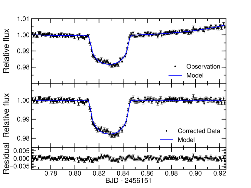
Figure 1: Top: a raw fractional light curve and the best-fit model light curve of GJ 1214 taken on 2012 August 12 UT with the Subaru Suprime-Cam in $B$-band. The model light curve includes both an analytic transit light curve and a baseline function. Middel: an OOT-normalized light curve and the best-fit transit light curve model. Bottom: residuals between the observed data and the best-fit model.

Table 2 summarizes the best-fit parameters and their uncertainties for each observation based on the MCMC analyses. As a result, we obtain the following planet-to-star radius ratios: $R_{\rm p}/R_{\rm s}=0.11651\pm 0.00065$ ($B$-band, Subaru/Suprime-Cam), $R_{\rm p}/R_{\rm s}=0.11601\pm 0.00117$ ($B$-band, Subaru/FOCAS), $R_{\rm p}/R_{\rm s}=0.11654\pm 0.00080$ ($J$-band, IRSF/SIRIUS), $R_{\rm p}/R_{\rm s}=0.11550^{+0.00142}_{-0.00153}$ ($H$-band, IRSF/SIRIUS), and $R_{\rm p}/R_{\rm s}=0.11547\pm 0.00127$ ($K_{\rm s}$-band, IRSF/SIRIUS). The observed light curves with the best-fit models for the Subaru and IRSF data are plotted in Figure 1 – 5. We also plot OOT-normalized light curves in Figure 1 – 5 for reference, although we fit the transit model and the baseline model simultaneously.

Overall, our observations indicate a flat transmission spectrum through $BJHK_{\rm s}$ bands. The transit depths do not appear significantly deeper in $B$- and $K_{\rm s}$-bands than $J$- or $H$-bands. The current IRSF/SIRIUS results are consistent with our previous ones with the same instrument (Narita et al., 2013), again refuting the deeper transit in $K_{\rm s}$-band. Our two $B$-band observations with Subaru Suprime-Cam and FOCAS are well consistent each other, however, we should note one thing as follows. In the residuals of Figure 1 ($B$-band, Subaru/Suprime-Cam), we see a small bump in the early half of the transit. The feature could be caused by a spot-crossing event. If the feature is truly a spot-crossing event, we can learn what effect the spot would have on Rp/Rs by eliminating the spot region from the data. For this purpose, we repeat the MCMC analysis using such data (specifically, data during 2456151.8194 – 2456151.8277 BJD_TDB are removed). Consequently we get $R_{\rm p}/R_{\rm s}=0.11882\pm 0.00070$ for this case. Although the feature is well consistent with a crossing over a small spot (a bump-height of $\sim$0.1% and a time-scale of $\sim$8 min: Carter et al. 2011; Berta et al. 2011), we cannot refute that it is a product of systematic effects. In addition, we should consider a possibility for a possible “hot-spot” (plage) occultation. Such a event may occur in stars with strong spot activity such as GJ 1214 (see e.g., Mohler-Fischer et al. 2013; Colon & Gaidos in prep.). For the current case, we removed only a possible spot-crossing region (with upward residuals), but there is a more subtle dip (downward residuals) just after the possible spot-crossing feature. As plages are typically located around dark spots, the slight dip may be caused by a plage crossing. If this is true, the above radius ratio ($R_{\rm p}/R_{\rm s}=0.11882\pm 0.00070$) should be considered as an upper limit. As we cannot decisively diagnose whether those features are real or not, the result with the Subaru Suprime-Cam should be treated with caution.

4.2 Stellar Variability

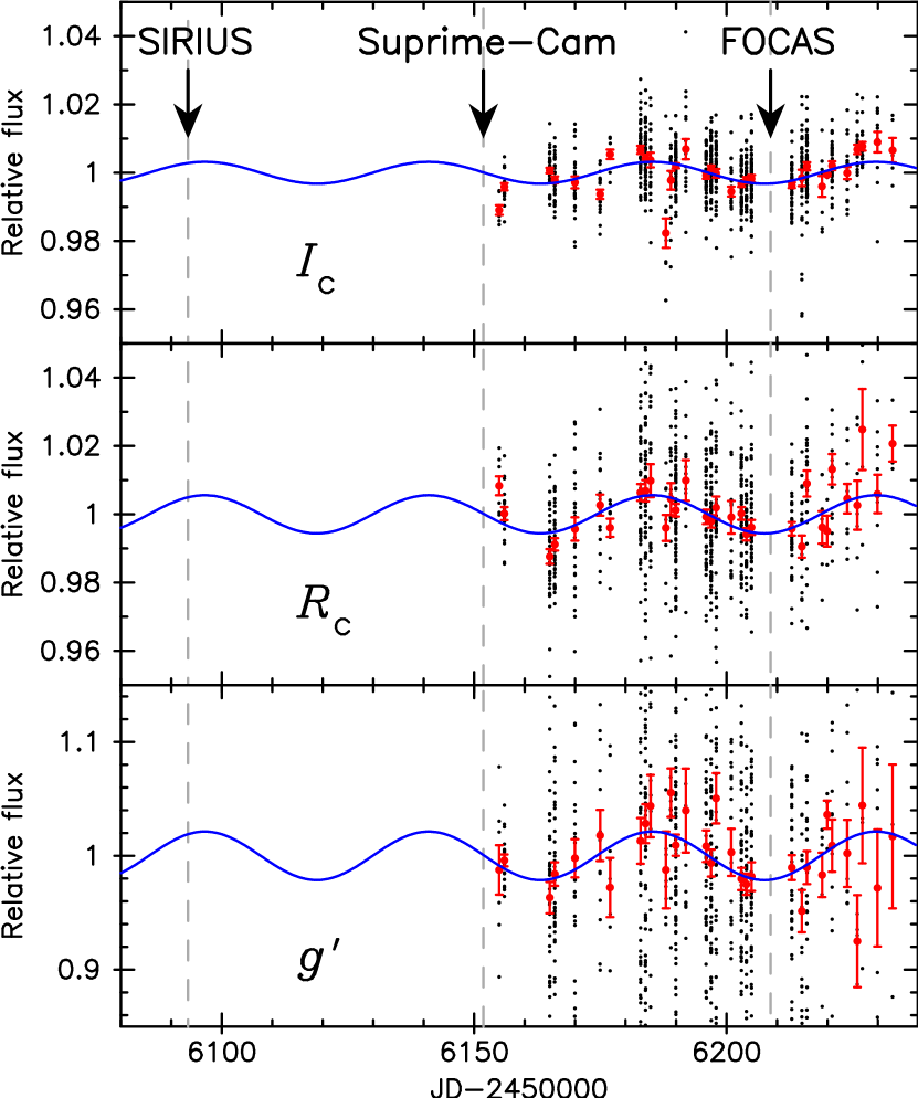
Figure 6: Long-term light curves of GJ 1214 obtained with the MITSuME 50cm telescope at the Okayama Astrophysical Observatory in 2012. The data were taken in three ($I_{\mathrm{c}}$: top, $R_{\mathrm{c}}$: middle, $g^{\prime}$: bottom) bands simultaneously. Observed data are plotted as dots. Data with error bars indicate mean values and rms divided by $\sqrt{N}$ values, where $N$ is the number of data points, of the observed data for each night for reference. Sinusoidal curves are the best-fit models based on the AMOEBA analysis described in section 3.2.

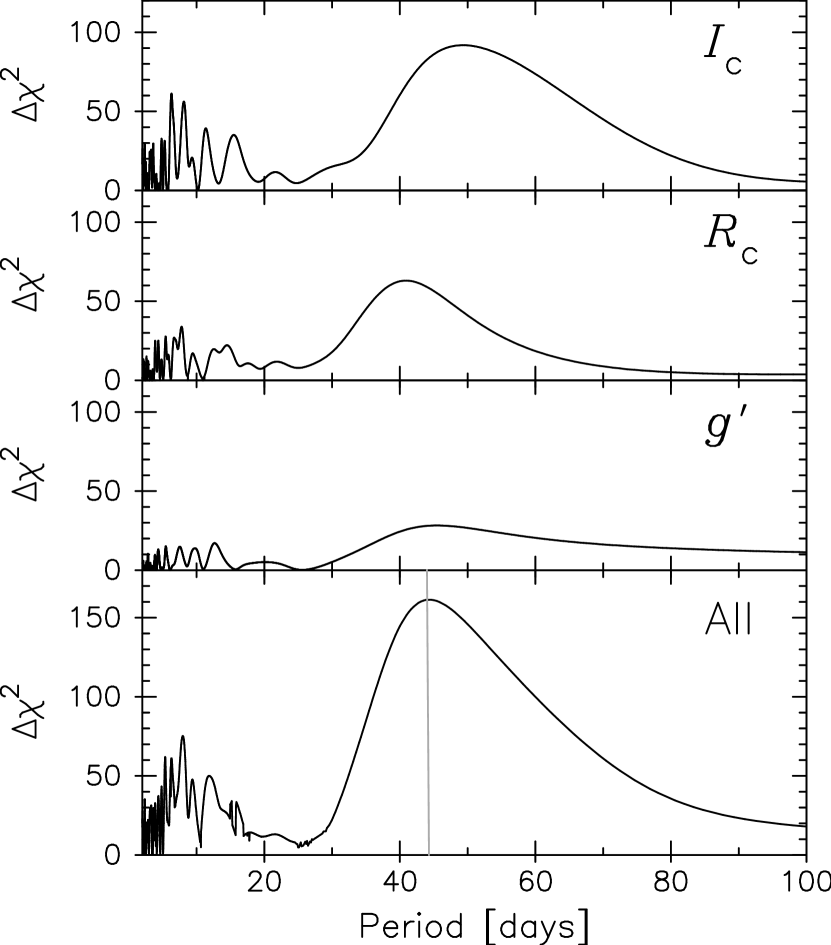
Figure 7: Periodograms for the MITSuME data. Results for $I_{\mathrm{c}}$-, $R_{\mathrm{c}}$-, $g^{\prime}$-bands, and a combined case are shown from top to bottom. The vertical axis indicates $\Delta\chi^{2}$ between the models for no variation ($A_{j}=0$) and for a fixed period at the horizontal axis (other parameters are free). The optimal case ($P_{\rm s}=44.3$ days) is indicated by the vertical line in the bottom panel.

Figure 6 plots the observed MITSuME data and the best-fit sinusoidal models. Figure 7 presents periodograms for the MITSuME data. Table 3 presents the best-fit values and their uncertainties for the free parameters. We obtain the lowest $\chi^{2}$ at the period of $P_{\rm s}=44.3$ days with an uncertainty of $\pm 1.2)$ days. The periodicity is a unique one (no other significant $\Delta\chi^{2}$ peak) in the observing span as we can see in figure 7. The estimated semi-amplitudes of the brightness variability are 0.32%$\pm$0.04% in $I_{\mathrm{c}}$-band, 0.56%$\pm$0.08% in $R_{\mathrm{c}}$-band, and 2.1%$\pm$0.4% in $g^{\prime}$-band. As we can see, the quality of the $g^{\prime}$-band data are relatively low (compared to the other bands) due to the faintness of the target. We thus note that the semi-amplitude of the $g^{\prime}$-band variability may be still inaccurate. Those results are very similar to the previous results by Berta et al. (2011), who reported 3.5 mmag brightness variability in $i+z$-band with a period of $\sim 53$ days and 7 mmag variability in $V$-band at a period of $\sim 41$ days.

To assess the significance of the variability, we calculate $\chi^{2}$ and BIC values for both the best-fit case and the null hypothesis case ($P$ and $t_{0}$ are removed from the model, and $A_{I_{\mathrm{c}}}$, $A_{R_{\mathrm{c}}}$, and $A_{g^{\prime}}$ are fixed to zero). We find $\Delta\chi^{2}=161.4$ and $\Delta$BIC = 122.0 ($\Delta k=5$ and $N=2646$). Thus the brightness variability is significantly detected, and our MITSuME monitoring independently confirms the stellar variability of GJ 1214. We caution, however, as Berta et al. (2011) mentioned, that the true rotation period of GJ 1214 could instead be a positive integer multiple of the quoted period. Since our monitoring covers only 78 nights, we cannot exclude a possibility of a longer stellar rotation period.

Even though the true stellar rotation period cannot be determined, the apparent stellar variability derived by our monitoring is useful to estimate and constrain systematic effects due to the stellar variability in the transit depths observed in 2012. In Figure 6, we show the observing dates of the transits, i.e., 2012 June 14 for the IRSF SIRIUS, 2012 August 12 for the Subaru Suprime-Cam, and 2012 October 8 for the Subaru FOCAS, with vertical lines. Since the MITSuME monitoring started after the Subaru Suprime-Cam observation, the phases for the IRSF SIRIUS observation and the Subaru Suprime-Cam observation are extrapolated by the period of $P_{\rm s}=44.3$ days. According to the figure, the brightness of GJ 1214 is nearly peak at the IRSF SIRIUS observation, middle at the Subaru Suprime-Cam observation, and bottom at the Subaru FOCAS observation.

4.3 Possible Impacts of Adopted Assumptions on Radius Ratios

We have adopted some assumptions in our analyses as shown in table 1. Since any large systematic effects would affect discussions on atmospheric models of GJ 1214b, we should check the robustness of our results against the assumptions. In the previous study, we have already confirmed the robustness of the radius ratios against $P$, $T_{\rm c,0}$, $i$, $a/R_{\rm s}$, and limb-darkening parameters in $JHK_{\rm s}$-bands (Narita et al., 2013). Thus a main concern for this study may arise from the assumption of the effective temperature and corresponding limb-darkening parameters of GJ 1214 in $B$-band. Indeed, Anglada-Escudé et al. (2013) recently reported a new parallax measurement for GJ 1214 that makes it appear that its effective temperature might be hotter than 3000 K (3252 K$\pm$20 K). Thus the adopted value of the limb-darkening parameters might become a source of a systematic effect.

To learn the level of the systematic effect and a possible dependence of radius ratios on the assumption of the effective temperature, we repeat the MCMC analyses for the $B$-band datasets for following 3 test cases: (1) $u_{1}$ is fixed to the value for $T_{\rm eff}=3000$ K and $u_{2}$ is free, (2) limb-darkening parameters with $T_{\rm eff}=3200$ K (specifically, $u_{1}=0.4749$ and $u_{2}=0.3666$: Claret & Bloemen 2011) are assumed, and (3) limb-darkening parameters with $T_{\rm eff}=2800$ K (specifically, $u_{1}=0.8687$ and $u_{2}=0.0996$: Claret & Bloemen 2011) are assumed.

For the case (1), we find $u_{2}=0.20\pm 0.06$ and $R_{\rm p}/R_{\rm s}=0.11728\pm 0.00088$ for the Subaru/Suprime-Cam data, while $u_{2}=0.30\pm 0.06$ and $R_{\rm p}/R_{\rm s}=0.11564^{+0.00150}_{-0.00157}$ for the Subaru/FOCAS data. The derived $u_{2}$ values are almost consistent with the empirical value of $u_{2}=0.2737$ (Claret & Bloemen, 2011), and the derived radius ratios are also consistent with the values reported in table 2 within 1$\sigma$. We additionally test an MCMC analysis with letting both $u_{1}$ and $u_{2}$ free, and find $R_{\rm p}/R_{\rm s}=0.11720\pm 0.00085$ for the Subaru/Suprime-Cam data, and $R_{\rm p}/R_{\rm s}=0.11548^{+0.00155}_{-0.00164}$ for the Subaru/FOCAS data. Those values are almost the same with the case (1), showing letting one limb-darkening parameter free is sufficient for this kind of tests. Based on this test, we estimate that the possible systematic effect due to the limb-darkening parameters is smaller than $\Delta(R_{\rm p}/R_{\rm s})\sim 0.001$, and we conclude that our results for radius ratios in $B$-band are robust. We also note that the above radius ratio values with free limb-darkening parameters do not change our conclusion in the section 4.5.

From the cases (2) and (3), we find an interesting trend between the radius ratio and the assumed effective temperature of GJ 1214. The derived radius ratios are $R_{\rm p}/R_{\rm s}=0.11803\pm 0.00065$ (case 2, Subaru/Suprime-Cam), $R_{\rm p}/R_{\rm s}=0.11838\pm 0.00123$ (case 2, Subaru/FOCAS), $R_{\rm p}/R_{\rm s}=0.11441\pm 0.00070$ (case 3, Subaru/Suprime-Cam), $R_{\rm p}/R_{\rm s}=0.11264\pm 0.00116$ (case 3, Subaru/FOCAS). Namely, an assumption of a hotter effective temperature gives a larger radius ratio, and vice versa. Among the assumed effective temperatures, the case for $T_{\rm eff}=3000$ K seems the most consistent with the test case (1), thus we do not change our main results. Although identifying a reason of this trend is beyond the scope of this paper, this kind of tests for the systematic effect due to the limb-darkening parameters would be necessary in future studies, especially in bluer wavelength regions.

4.4 Possible Impacts of Unocculted Starspots on Radius Ratios

Unocculted starspots are known to cause a systematic effect on an apparent radius ratio (see e.g., Carter et al. 2011; Désert et al. 2011b; Sing et al. 2011). The systematic difference of the radius ratio $\Delta(R_{\rm.p}/R_{\rm s})$ caused by the stellar variability due to starspots can be written as

$$\Delta(R_{\rm p}/R_{\rm s})\simeq 0.5\,\,\Delta f(\lambda)\,\,(R_{\rm p}/R_{\rm s}),$$ (1)

where $\Delta f(\lambda)$ is stellar brightness variability at wavelength $\lambda$ (Sing et al., 2011; Narita et al., 2013).

The brightness of GJ 1214 in $g^{\prime}$-band on the two observing nights of the Subaru Suprime-Cam and the Subaru FOCAS is different by $\sim$2% based on the MITSuME monitoring, and given that the semi-amplitude of the stellar variability in $B$-band is similar to that in $g^{\prime}$-band, a systematic difference between the Subaru Suprime-Cam and the Subaru FOCAS observations is $\Delta(R_{\rm p}/R_{\rm s})\sim 0.0012$. However, this value may be too conservative, since the semi-amplitude of the $g^{\prime}$-band variability may be inaccurate due to poor signal-to-noise ratio, as we have cautioned in the previous section, and since it appears to be much larger than the semi-amplitude in $V$-band ($\sim 7$ mmag) reported by Berta et al. (2011). For this reason, we also try an independent simple estimate for the effect of unocculted spots in $B$-band as follows. First, we assume the temperatures of the (normal) stellar surface and the spot region to be $T_{\rm star}=3000$ K and $T_{\rm spot}=2700$ K. Assuming the black-body profile for the emission from those regions, we search for an optimal spot coverage that can explain the semi-amplitude of $R_{\mathrm{c}}$- and $I_{\mathrm{c}}$-band variability. We find that a spot coverage of 0.73% gives the best-fit for those two bands. Using this value, the semi-amplitude of the stellar variability in $B$-band is estimated as 0.88% and the possible systematic difference in the radius ratio is $\Delta(R_{\rm p}/R_{\rm s})\sim 0.00053$ at most. In either case, we estimate a possible systematic effect on the radius ratio in $B$-band is as small as or smaller than $\Delta(R_{\rm p}/R_{\rm s})\sim 0.001$.

We note that the more unocculted spots exist, the deeper transits would be observed (Carter et al., 2011). Namely the transit at the time of the FOCAS observation is expected to be the deepest. Our results shown in Table 2, however, appear to be inverse, but this is not significant when considering the uncertainties in $R_{\rm p}/R_{\rm s}$ for the Suprime-Cam and the FOCAS observations.

For the near-infrared region, if we suppose that the semi-amplitude of the stellar variability in the near-infrared region is similar or smaller than the variability in $I_{\mathrm{c}}$-band from the MITSuME monitoring, then the difference of the stellar brightness in $JHK_{\rm s}$-bands is less than $\sim$0.6%. Based on this assumption, we estimate maximum systematic differences of radius ratios in $JHK_{\rm s}$-bands are $\Delta(R_{\rm p}/R_{\rm s})\leq 0.0004$, which is well smaller than the observational uncertainties. On the other hand, if we again adopt the same estimation method used for $B$-band, we derive the semi-amplitudes of the stellar variability in $JHK_{\rm s}$-bands as 0.20%, 0.15%, and 0.12%, respectively. Those values are consistent with the above assumption. Based on the values, we estimate possible systematic effects on the radius ratio as $\Delta(R_{\rm p}/R_{\rm s})\sim 0.00012(J),0.00009(H),$ and $0.00007(K_{\rm s})$, respectively. Thus we conclude that we can neglect systematic effects due to unocculted spots in the near-infrared region within the current observational errors.

4.5 Atmospheric Models

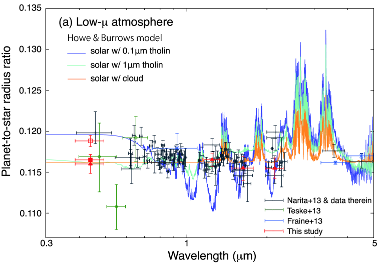
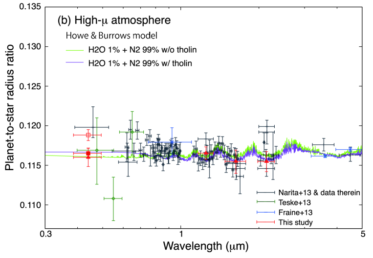
Figure 8: Measured planet-to-star radius ratios vs. wavelength in microns for GJ 1214b, compared with the five best-fit theoretical spectra from Howe & Burrows (2012). The same set of observation data is shown in panel (a) and (b). In (a), the theoretical spectra for the solar-abundance atmosphere are shown, while those for the water-rich atmosphere are shown in (b). As for the $B$-band, the filled triangle and square represent the data obtained with the FOCAS and the Suprime-Cam, while the open square does the case for the Suprime-Cam without possible spot-crossing data.

Measured radius ratios of GJ 1214b published so far are plotted with respect to wavelength in Figure 8, which also shows the five best-fit spectra from the Figure 21 of Howe & Burrows (2012). As described in Section 1, Narita et al. (2013) raised a possibility of a high molecular weight (high-$\mu$), vapor-rich atmosphere which predicts a flat spectrum, by showing that a $K_{\rm s}$-band transit was shallower than those from Croll et al. (2011) and de Mooij et al. (2012). The new $K_{s}$-band transit depth from the IRSF SIRIUS observation is consistent with the previous values of ours and Bean et al. (2011). This does not mean, however, that another possibility of a low-$\mu$, hydrogen-dominated atmosphere is excluded when considering extensive clouds. This is because both theoretical spectra of the high-$\mu$ and low-$\mu$ atmospheres yield similar transit depths at the $K_{s}$-band wavelength, as seen in Figure 8a.

The $B$-band transit that we have observed with the Subaru FOCAS is significantly shallower than the $g$-band transit reported by de Mooij et al. (2012). As discussed in Howe & Burrows (2012), the deep $g$-band transit needs a Rayleigh-scattering-like feature (the Rayleigh slope) in the visible to near-infrared wavelength region, which appears in the theoretical spectrum of a hydrogen-rich atmosphere with tholin haze (see Figure 8a). In contrast, the shallow $B$-band transit is consistent with the model spectra for high-$\mu$ atmospheres without the Rayleigh slope (see Figure 8b). Among the five best-fit models proposed by Howe & Burrows (2012), the model spectra for the 1% H₂O + 99% N₂ atmosphere (with and without tholin haze) appear most likely. While the solar-composition (low-$\mu$) atmosphere with opaque clouds may also account for the FOCAS $B$-band transit as well as the IRSF $JHK_{\rm s}$-band transits. In contrast, the low-$\mu$ atmosphere with 0.1$\mu$m tholin haze is inconsistent with the FOCAS $B$-band transit, and the similar atmosphere with 1$\mu$m tholin haze is also inconsistent with the IRSF $HK_{\rm s}$-band transits.

Unfortunately, the result from the Suprime-Cam is inconclusive due to the possible spot-crossing event, as discussed in the section 4.1. Given the spot-crossing is real, the difference of the transit depths between the two observations ($R_{\rm p}/R_{\rm s}{\rm(Suprime-Cam)}=0.11882\pm 0.00070$ and $R_{\rm p}/R_{\rm s}{\rm(FOCAS)}=0.11601\pm 0.00117$) is about 2$\sigma$ (1$\sigma$ here is a square-root of sum of squares of both uncertainties). Although the significance of the difference is marginal, the two transit depths appears to be inconsistent. One possibility to explain the difference is that the stellar activity might cause a temporal change in the amount of haze in the atmosphere. In the case of Titan’s atmosphere, it is known that the solar UV flux and Saturn’s magnetospheric electrons and protons contribute to synthesize tholin haze (Khare et al., 1984). When a close-in planet like GJ 1214b passes through a stellar-spot magnetosphere, the production rate of tholin haze might be affected. A time variation in the amount of tholin haze might lead to the change of the $B$-band transit depths. In this case, some amount of a low-$\mu$ component should be present in the atmosphere of GJ 1214b. Although it is highly speculative, this possibility is worth exploring by repeated future observations.

Whether the atmosphere contains a significant amount of water or not affects our understanding of the origin of GJ 1214b. The deep photometric transit originally presented by Charbonneau et al. (2009) suggests that GJ 1214b contains some low-$\mu$ components. If the planet is completely differentiated, it must be enveloped with a low-$\mu$ atmosphere. Within the context of the core-accretion model, a hydrogen-rich atmosphere of nebular origin is the most-likely possibility (Ikoma & Hori, 2012). Detailed modeling of the internal structure of GJ 1214b (Nettelmann et al., 2011; Valencia et al., 2013) predicts that the hydrogen-rich atmosphere constitutes several % of the planet mass to reproduce the mass-radius relationship for this planet. It should be also noted that recently Morley et al. (2013) suggested that cloud and hydrocarbon haze formation in the atmosphere of GJ 1214b by (non-)equilibrium chemistry favored atmospheric models with enhanced metallicity.

The atmosphere of GJ 1214b may have been subject to photo-evaporative mass loss due to stellar XUV irradiation. Although the current irradiation level would be so low that the atmosphere will undergo no significant mass loss today and in the future, several studies advocated that a GJ 1214b-like planet had experienced a significant removal of the atmosphere in the past (e.g. Owen & Wu 2013). The mass loss history is, however, not well-constrained, because we do not know the current intrinsic luminosity of GJ 1214b, which affects the speed of the thermal evolution significantly. Thus, we cannot deny the presence of such a hydrogen-rich atmosphere theoretically from the viewpoint of the internal structure and evolution.

On the other hand, absence of low-$\mu$ components in the atmosphere would give some important constraints on the structure and origin of this planet. To reconcile with the planet’s low-density, one possibility would be that low-$\mu$ components should be incorporated in the interior; for example, the envelope in the mixed state with water and H/He. Giant collisions between super-Earths or heavy secondary bombardments of volatile-rich planetesimals would be needed for such mixing to occur. Such processes triggered in a planetary system would lead to form multiple planets. Provided that this picture holds true for GJ 1214b, we predict that additional planets should exist in the GJ 1214 system. Thus search for outer planets helps us to learn the formation history of GJ 1214b.

4.6 Suggestions for Future Observations

Although our results have suggested that GJ 1214b has a fairly flat transmission spectrum through $BJHK_{\rm s}$-bands, it is still difficult to determine one decisive atmosphere model. Experiences have shown that broadband single-color transit photometry is not efficient to constrain an atmosphere model in the presence of starspots and the stellar variability. More effective ways to characterize atmospheres of transiting planets would be (1) simultaneous multi-band transit photometry using small-medium ground-based telescopes (e.g., Croll et al. 2011; de Mooij et al. 2012; Narita et al. 2013; Fukui et al. 2013b), (2) multi-object spectro-photometry using large ground-based telescopes (e.g., Bean et al. 2010, 2011), and (3) spectro-photometry using space telescopes (e.g., Berta et al. 2012). It would be important to observe the wavelength region where the difference of transit depths between the low-$\mu$ and the high-$\mu$ atmospheres is significant, especially the Rayleigh slope (optical) region and around $K$-band region. In addition, repeated transit observations are highly desirable to improve the significance and to check possible time variations. As the ongoing ground-based transit surveys (e.g., MEarth) and the future space-based survey like TESS (Ricker et al., 2010) will discover more transiting super-Earths around nearby cool host stars, the current experiences for GJ 1214b would become a good practice for the future.

5 Summary

We have presented two $B$-band transits observed with the Suprime-Cam and FOCAS on the Subaru 8.2m telescope and one simultaneous $JHK_{\rm s}$-band transit taken with the SIRIUS camera on the IRSF 1.4m telescope. Our measurements of transit depths suggest a fairly flat transmission spectrum through $BJHK_{\rm s}$-bands. Comparisons of our new results and previous observations with theoretical atmospheric models from Howe & Burrows (2012) indicate that the high-$\mu$ (water-rich) atmosphere models are most likely, although the low-$\mu$ (hydrogen-dominated) atmosphere with thick clouds may still account for the observations. As noted in section 4.1., our Subaru Suprime-Cam data show a possible spot-crossing event. Suppose that the spot-crossing is real and the data from the event is removed, our two $B$-band results are marginally inconsistent. It is slightly puzzling, but it may be simply due to unknown systematic effects, or it may be explained by temporal changes of transit depths due to the stellar activity and thereby time variations of haze amount. To further constrain the atmosphere model of GJ 1214b and to check a possibility of the presence of time variations in transit depths or the Rayleigh slope, more repeated observations described in the previous subsection (section 4.6.) would be desirable in the future.

Table 1: Assumed parameters and their sources.

Parameter	Value	Source
$P$ [days]	1.58040481	Bean et al. (2011)
$T_{\rm c,0}$ [BJDTDB]	2454966.525123	Bean et al. (2011)
$i$ [∘]	88.94	Bean et al. (2010)
$a/R_{\rm s}$	14.9749	Bean et al. (2010)
$u_{\rm 1,B}$	0.6366	Claret & Bloeman (2011)
$u_{\rm 2,B}$	0.2737	Claret & Bloeman (2011)
$u_{\rm 1,J}$	0.0875	Claret & Bloeman (2011)
$u_{\rm 2,J}$	0.4043	Claret & Bloeman (2011)
$u_{\rm 1,H}$	0.0756	Claret & Bloeman (2011)
$u_{\rm 2,H}$	0.4070	Claret & Bloeman (2011)
$u_{\rm 1,Ks}$	0.0475	Claret & Bloeman (2011)
$u_{\rm 2,Ks}$	0.3502	Claret & Bloeman (2011)
$T_{\rm eff}$ [K]	3000	Croll et al. (2011)
$\log g$	5.0	Croll et al. (2011)

Table 2: Best-fit values and uncertainties for the parameters of the transit light curves based on the MCMC analyses.

Parameter	Value	Uncertainty
Subaru/Suprime-Cam (2012 August 12)
$R_{\rm p}/R_{\rm s}$ (B)	0.11651	$\pm 0.00065$
$k_{0}$	0.98676	$\pm 0.00099$
$k_{t}$	-0.0110	$\pm 0.0018$
$k_{z}$	0.00494	$\pm 0.00036$
$\Delta r$	17	–
Subaru/Suprime-Cam (spot-feature removed)
$R_{\rm p}/R_{\rm s}$ (B)	0.11882	$\pm 0.00070$
$k_{0}$	0.98712	$\pm 0.00092$
$k_{t}$	-0.0104	$\pm 0.0016$
$k_{z}$	0.00482	$\pm 0.00033$
$\Delta r$	17	–
Subaru/FOCAS (2012 October 8)
$R_{\rm p}/R_{\rm s}$ (B)	0.11601	$\pm 0.00117$
$k_{0}$	0.9780	$\pm 0.0011$
$k_{t}$	-0.0373	$\pm 0.0075$
$k_{z}$	0.00642	$\pm 0.00039$
$k_{s}$ ($\times 10^{-7}$)	-1.45	$\pm 0.37$
$\Delta r$	18	–
IRSF/SIRIUS (2012 June 14)
$R_{\rm p}/R_{\rm s}$ (J)	0.11654	$\pm 0.00080$
$k_{0}$	1.00119	$\pm 0.00012$
$k_{t}$	0.0128	$\pm 0.0015$
$\Delta r$	17	–
IRSF/SIRIUS (2012 June 14)
$R_{\rm p}/R_{\rm s}$ (H)	0.11550	${}^{+0.00142}_{-0.00153}$
$k_{0}$	0.9835	$\pm 0.0074$
$k_{t}$	0.025	$\pm 0.012$
$k_{z}$	0.0052	$\pm 0.0022$
$k_{x}$ ($\times 10^{-4}$)	1.86	$\pm 0,49$
$\Delta r$	17	–
IRSF/SIRIUS (2012 June 14)
$R_{\rm p}/R_{\rm s}$ (Ks)	0.11547	$\pm 0.00127$
$k_{0}$	0.9856	$\pm 0.0014$
$k_{z}$	0.00495	$\pm 0.00042$
$\Delta r$	16	–

Table 3: Best-fit values and uncertainties for the parameters of the Sinusoidal Variability of GJ1214.

Parameter	Value	Uncertainty
$P_{s}$ [days]	44.3	$\pm 1.2$
$t_{0}$ [JD-2,450,000]	6174.22	${}^{+0.77}_{-0.81}$
$A_{I_{\mathrm{c}}}$	0.00319	$\pm 0.00038$
$A_{R_{\mathrm{c}}}$	0.00558	$\pm 0.00078$
$A_{g^{\prime}}$	0.0213	$\pm 0.0042$
$k_{0,I_{\mathrm{c}}}$	0.9958	$\pm 0.0015$
$k_{0,R_{\mathrm{c}}}$	0.9729	$\pm 0.0031$
$k_{0,g^{\prime}}$	1.0405	${}^{+0.0158}_{-0.0166}$
$k_{z,I_{\mathrm{c}}}$	-0.0028	$\pm 0.0011$
$k_{z,R_{\mathrm{c}}}$	-0.0210	$\pm 0.0023$
$k_{z,g^{\prime}}$	0.0262	${}^{+0.0127}_{-0.0119}$

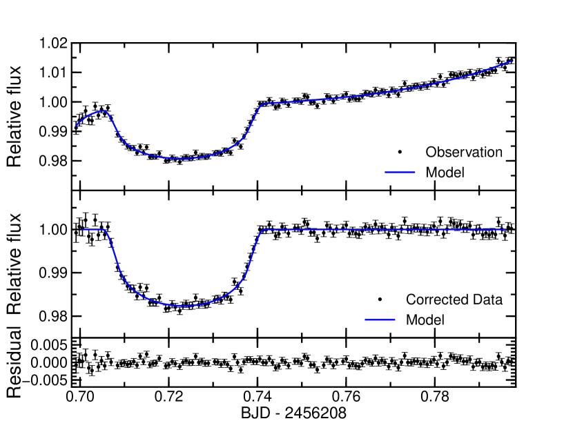
Figure 2: Same as figure 1, but for the data taken on 2012 October 8 UT, with the Subaru FOCAS in $B$-band.

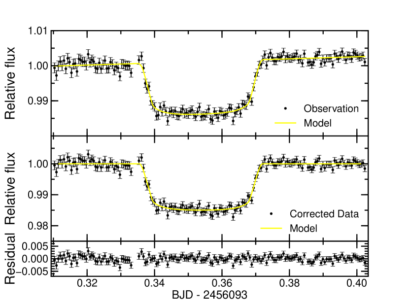
Figure 3: Same as figure 1, but for the data taken on 2012 June 14 UT, with the IRSF SIRIUS in $J$-band.

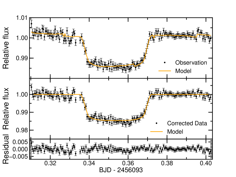
Figure 4: Same as figure 3, but for the data taken in $H$-band.

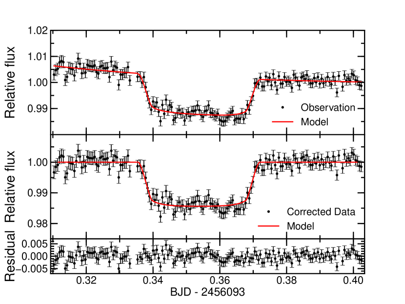
Figure 5: Same as figure 3, but for the data taken in $K_{\rm s}$-band.

References

- Adelman-McCarthy & et al. (2011) Adelman-McCarthy, J. K., & et al. 2011, VizieR Online Data Catalog, 2306, 0
- Anglada-Escudé et al. (2013) Anglada-Escudé, G., Rojas-Ayala, B., Boss, A. P., Weinberger, A. J., & Lloyd, J. P. 2013, A&A, 551, A48
- Bean et al. (2010) Bean, J. L., Miller-Ricci Kempton, E., & Homeier, D. 2010, Nature, 468, 669
- Bean et al. (2011) Bean, J. L., et al. 2011, ApJ, 743, 92
- Benneke & Seager (2012) Benneke, B., & Seager, S. 2012, ApJ, 753, 100
- Berta et al. (2011) Berta, Z. K., Charbonneau, D., Bean, J., Irwin, J., Burke, C. J., Désert, J.-M., Nutzman, P., & Falco, E. E. 2011, ApJ, 736, 12
- Berta et al. (2012) Berta, Z. K., et al. 2012, ApJ, 747, 35
- Carter et al. (2011) Carter, J. A., Winn, J. N., Holman, M. J., Fabrycky, D., Berta, Z. K., Burke, C. J., & Nutzman, P. 2011, ApJ, 730, 82
- Charbonneau et al. (2009) Charbonneau, D., et al. 2009, Nature, 462, 891
- Claret & Bloemen (2011) Claret, A., & Bloemen, S. 2011, A&A, 529, A75
- Croll et al. (2011) Croll, B., Albert, L., Jayawardhana, R., Miller-Ricci Kempton, E., Fortney, J. J., Murray, N., & Neilson, H. 2011, ApJ, 736, 78
- Cutri et al. (2003) Cutri, R. M., et al. 2003, 2MASS All Sky Catalog of point sources., ed. Cutri, R. M., Skrutskie, M. F., van Dyk, S., Beichman, C. A., Carpenter, J. M., Chester, T., Cambresy, L., Evans, T., Fowler, J., Gizis, J., Howard, E., Huchra, J., Jarrett, T., Kopan, E. L., Kirkpatrick, J. D., Light, R. M., Marsh, K. A., McCallon, H., Schneider, S., Stiening, R., Sykes, M., Weinberg, M., Wheaton, W. A., Wheelock, S., & Zacarias, N.
- de Mooij et al. (2012) de Mooij, E. J. W., et al. 2012, A&A, 538, A46
- Désert et al. (2011a) Désert, J.-M., et al. 2011a, ApJ, 731, L40
- Désert et al. (2011b) Désert, J.-M., et al. 2011b, A&A, 526, A12
- Eastman et al. (2010) Eastman, J., Siverd, R., & Gaudi, B. S. 2010, PASP, 122, 935
- Fraine et al. (2013) Fraine, J. D., et al. 2013, ApJ, 765, 127
- Fukui et al. (2011) Fukui, A., et al. 2011, PASJ, 63, 287
- Fukui et al. (2013b) Fukui, A., et al. 2013, ApJ, 770, 95
- Gelman & Rubin (1992) Gelman, A., & Rubin, D. 1992, Statistical Science, 7, 457
- Howe & Burrows (2012) Howe, A. R., & Burrows, A. S. 2012, ApJ, 756, 176
- Ikoma & Hori (2012) Ikoma, M., & Hori, Y. 2012, ApJ, 753, 66
- Kashikawa et al. (2002) Kashikawa, N., et al. 2002, PASJ, 54, 819
- Khare et al. (1984) Khare, B. N., Sagan, C., Arakawa, E. T., Suits, F., Callcott, T. A., & Williams, M. W. 1984, Icarus, 60, 127
- Kotani et al. (2005) Kotani, T., et al. 2005, Nuovo Cimento C Geophysics Space Physics C, 28, 755
- Mandel & Agol (2002) Mandel, K., & Agol, E. 2002, ApJ, 580, L171
- Miller-Ricci & Fortney (2010) Miller-Ricci, E., & Fortney, J. J. 2010, ApJ, 716, L74
- Miyazaki et al. (2002) Miyazaki, S., et al. 2002, PASJ, 54, 833
- Mohler-Fischer et al. (2013) Mohler-Fischer, M., et al. 2013, ArXiv e-prints
- Morley et al. (2013) Morley, C. V., Fortney, J. J., Kempton, E. M.-R., Marley, M. S., Visscher, C., & Zahnle, K. 2013, ArXiv e-prints
- Nagayama et al. (2003) Nagayama, T., et al. 2003, in Society of Photo-Optical Instrumentation Engineers (SPIE) Conference Series, Vol. 4841, Society of Photo-Optical Instrumentation Engineers (SPIE) Conference Series, ed. M. Iye & A. F. M. Moorwood, 459–464
- Narita et al. (2013) Narita, N., Nagayama, T., Suenaga, T., Fukui, A., Ikoma, M., Nakajima, Y., Nishiyama, S., & Tamura, M. 2013, PASJ, 65, 27
- Narita et al. (2007) Narita, N., et al. 2007, PASJ, 59, 763
- Nettelmann et al. (2011) Nettelmann, N., Fortney, J. J., Kramm, U., & Redmer, R. 2011, ApJ, 733, 2
- Ohta et al. (2009) Ohta, Y., Taruya, A., & Suto, Y. 2009, ApJ, 690, 1
- Owen & Wu (2013) Owen, J. E., & Wu, Y. 2013, ArXiv e-prints
- Pont et al. (2006) Pont, F., Zucker, S., & Queloz, D. 2006, MNRAS, 373, 231
- Press et al. (1992) Press, W. H., Teukolsky, S. A., Vetterling, W. T., & Flannery, B. P. 1992, Numerical recipes in C. The art of scientific computing (Cambridge: University Press, —c1992, 2nd ed.)
- Ricker et al. (2010) Ricker, G. R., et al. 2010, in Bulletin of the American Astronomical Society, Vol. 42, American Astronomical Society Meeting Abstracts #215, #450.06
- Schwarz (1978) Schwarz, G. 1978, Ann. Statistics, 6, 461
- Sing et al. (2011) Sing, D. K., et al. 2011, MNRAS, 416, 1443
- Teske et al. (2013) Teske, J. K., Turner, J. D., Mueller, M., & Griffith, C. A. 2013, MNRAS, 431, 1669
- Valencia et al. (2013) Valencia, D., Guillot, T., Parmentier, V., & Freedman, R. S. 2013, ArXiv e-prints
- Yanagisawa et al. (2010) Yanagisawa, K., Kuroda, D., Yoshida, M., Shimizu, Y., Nagayama, S., Toda, H., Ohta, K., & Kawai, N. 2010, in American Institute of Physics Conference Series, Vol. 1279, American Institute of Physics Conference Series, ed. N. Kawai & S. Nagataki, 466–468
- Winn et al. (2008) Winn, J. N., et al. 2008, ApJ, 683, 1076