Cluster Probes of Dark Energy Clustering

Abstract

Cluster abundances are oddly insensitive to canonical early dark energy. Early dark energy with sound speed equal to the speed of light cannot be distinguished from a quintessence model with the equivalent expansion history for $z<2$ but negligible early dark energy density, despite the different early growth rate. However, cold early dark energy, with a sound speed much smaller than the speed of light, can give a detectable signature. Combining cluster abundances with cosmic microwave background power spectra can determine the early dark energy fraction to 0.3% and distinguish a true sound speed of 0.1 from 1 at 99% confidence. We project constraints on early dark energy from the Euclid cluster survey, as well as the Dark Energy Survey, using both current and projected Planck CMB data, and assess the impact of cluster mass systematics. We also quantify the importance of dark energy perturbations, and the role of sound speed during a crossing of $w=-1$.

I Introduction

Understanding the physics behind cosmic acceleration requires clear characterization of the properties of dark energy. This includes its dynamics, e.g. equation of state behavior $w(z)$, its degrees of freedom, e.g. perturbations or sound speed $c_{s}(z)$, and its persistence, i.e. presence of dark energy at high redshift. Distance measurements are most sensitive to the first of these properties suzuki ; wigglez ; boss . Cosmic microwave background (CMB) data can constrain the second and third to some extent 2003MNRAS.346..987W ; 2004PhRvD..69h3503B ; 09010916 ; dhl ; 10105612 ; 11034132 ; 11105328 ; 11060299 in particular if correlated with large scale structure observations. Growth of large scale structure might be expected to also be affected by perturbations and early dark energy doranrob ; Wetterich04 ; fll1 ; grossi ; fll2 ; dhl ; alam , but normalization to the present growth amplitude or abundance removes almost all this sensitivity fll1 .

For perturbations in the dark energy to have an appreciable influence on the matter power spectrum and large scale clustering, two conditions are necessary. The first is that the dark energy equation of state, or pressure to density, ratio $w$ must be significantly different from $-1$, the cosmological constant value, since the influence of perturbation enters with a prefactor $1+w$ (see dhl for analytic scalings). Since data constraints indicate that at low redshift $w\approx-1$, we need persistence of dark energy to high redshift, where $w$ can be significantly different from $-1$, approaching $w\approx 0$. Thus we talk about early dark energy, that may have a fraction of the critical density $\Omega_{de}(z_{lss})\approx 10^{-2}$ at the CMB last scattering surface rather than $\Omega_{\Lambda}(z_{lss})\approx 10^{-9}$.

The second requirement is that the sound horizon $c_{s}H^{-1}$ of the dark energy perturbations be well within the Hubble scale $H$. Dark energy clusters only on scales outside its sound horizon and smaller than the Hubble scale, $H<k<H/c_{s}$, where $k$ is the perturbation wavemode, in the same way that matter clumps only on scales greater than its own Jeans scale. Thus, inclusion of dark energy perturbations per se is not the key, but perturbations that can grow. Therefore we require that the sound speed be small compared to the speed of light, $c_{s}\ll 1$. This is referred to as cold dark energy 10072188 ; 10105612 . In this article we explore signatures of cold early dark energy on galaxy cluster abundances.

In Sec. II we discuss the influence of dark energy in terms of its expansion history and perturbations, especially on the matter power spectrum and cluster mass function. We compute the cluster abundances in Sec. III in different models for forthcoming surveys to determine the signal to noise of the dark energy signature. Including cosmological parameter and observational systematics covariance in Sec. IV we project constraints on the dark energy properties.

II Dark Energy Effects on Matter Clustering

Dark energy acts to suppress the growth of matter structures through increasing the Hubble friction and reducing the matter source term (see, e.g., linjen for detailed discussion). Early dark energy, through its persistence to higher redshifts, strengthens the suppression. Even if at early times the dark energy has $w\approx 0$, i.e. acts roughly like matter in the expansion, the reduction in the source term for matter perturbations causes suppression.

Of course the dark energy itself has perturbations, as any fluid with $w\neq-1$ must, but these generally provide negligible contribution to the Poisson term sourcing the matter perturbations. For example, dhl ; 10045509 show that for a canonical sound speed $c_{s}=1$, the ratio of the dark energy perturbation power spectrum to the matter power spectrum goes as $(k/H)^{-4}$. Even at wavemode $k=0.01\,h$/Mpc, only accessible to very large scale structure surveys, dark energy only contributes $\sim 10^{-8}$ as much power as matter does. Therefore canonical dark energy, even early dark energy, has negligible effect on the matter growth, power spectrum, or cluster abundances other than through its expansion effects on the growth. If this is normalized out by fixing the mass fluctuation amplitude $\sigma_{8}$ today, then there is remarkable insensitivity to the presence of early dark energy.

This was demonstrated in detail through computing the matter power spectrum and halo mass function (HMF) from N-body simulations and showing their close agreement with $\Lambda$CDM computations fll1 . This was also seen for the HMF for a different early dark energy model in grossi , assuming the $\Lambda$CDM linear collapse threshold $\delta_{c}$ within the spherical collapse formalism, and fll2 derived that $\delta_{c}$ is indeed near the $\Lambda$CDM value. The insensitivity is robust to the manner of identifying halos and the specific mass function used. At redshifts $z>0$, few-tens of percent level deviations can arise in cluster abundances with mass $M>10^{14}M_{\odot}/h$ due to the differing growth histories fll1 . The internal structure of clusters, e.g. their concentrations, could also show signs of the differing growth history of early dark energy grossi .

Differences in the HMF within another early dark energy model were found in alam but this is due to strongly differing values of the present matter fluctuations, i.e. $\sigma_{8}$. It is not due to the inclusion of dark energy perturbations; note that fll1 included perturbations in the initial linear power spectrum of the simulations and as mentioned above dhl calculated the effect of perturbations and found them to be negligible for canonical dark energy. These results leave open the possibility that cold early dark energy could give detectable effects on the HMF (dhl found signatures from it in the matter and CMB power spectra). We investigate this in the next section. In general we should note that a cold early dark energy component is expected to be more inhomogenous then a component with a sound speed of $c_{s}=1$. On the non-linear level this could lead to stronger backreaction effects also on the matter distribution and hence altering the HMF on a level beyond the one included in the change of the linear matter power spectrum. However in order to simulate this effect properly we would need to include the scalar field on a grid in N-body simulations. This is an extremely demanding task, which so far has only been addressed in the context of scalar-tensor theories Oyaizu:08 ; Li:12 ; Puchwein:13 . We follow the approach to only include the changes in the linear power spectrum and propagate to the nonlinear regime in the standard way as described below. We expect that this will result in conservative constraints, which might be tighter once the full nonlinear behaviour is taken into account.

III Cluster Mass Function Signals

The halo mass function is generally calculated from a fitting form that is a function of the linear mass fluctuation amplitude on the scale corresponding to the cluster mass, $\sigma(M,z)$. A popular modern form, adopted here, is the Tinker et al. tinker mass function,

$$\frac{dn}{dM} = f(\sigma)\,\frac{\bar{\rho}_{m}}{M}\frac{d\ln\sigma^{-1}}{dM}$$ (1)

$$f(\sigma) = A\left[\left(\frac{\sigma}{b}\right)^{-d}+1\right]\,e^{-c/\sigma^{2}}$$ (2)

$$\sigma^{2}(M,z) = 4\pi\int dk\,k^{2}\,P(k,z)\,W^{2}(kR)\ ,$$ (3)

where $n$ is the cluster abundance, $f$ is the multiplicity function, $P$ is the linear matter power spectrum, and $W$ is the window function on scale $R$ corresponding to mass $M$.

The linear power spectrum for a dark energy model, cold and early or not, can be calculated from a modified version of CAMB camb . This includes perturbations in the dark energy; see the discussion later of their special importance for cold early dark energy.

The Tinker et al. mass function has been investigated for universality with respect to cosmology, however not for early dark energy models. As mentioned above, one would need to carry out involved N-body simulations of each such model, including dark energy fields to follow their perturbations (and testing halo identification with respect to virialization). On the other hand, fll1 ; grossi showed that older mass functions such as Jenkins et al. jenkins , Sheth-Tormen shethtormen , and Warren et al. warren , while also calibrated from $\Lambda$, still agreed as well with N-body simulations of early dark energy cosmologies. Furthermore, fll2 demonstrated that the linear collapse threshold for early dark energy, as enters the Sheth-Tormen and similar excursion set approaches, was quite similar to $\Lambda$CDM. For low sound speed, the clustering of the dark energy fluid makes it act more like standard matter, and hence this is even more true as computed by pace , and so the mass function form should be even more acceptable, although a final verdict requires the inclusion of an inhomogenous cold early dark energy component in the simulations. For conservative reasons we assume the Tinker et al. HMF holds for the cold early dark energy models, with the same constant coefficients given in tinker ; we note that this HMF is commonly used in the literature for non-$\Lambda$CDM cosmologies, although eventually simulations should verify the level of universality.

The signal to noise of a cold early dark energy component in the cluster mass function is given by the deviation of the abundance relative to a fiducial model, say, $\Lambda$CDM with the same cosmological parameters other than those for dark energy,

$$\frac{S}{N}=\frac{N_{\rm model}-N_{\rm fid}}{\delta N_{\rm model}}\ ,$$ (4)

where this can be evaluated for each mass bin and redshift bin (or summed in quadrature over them), and $\delta N$ represents the measurement uncertainty of the cluster abundance (e.g. Poisson error) within the bin.

Survey characteristics enter through the mass threshold, below which clusters cannot be detected, redshift range, and the Poisson error that follows from the survey volume (as well as systematic uncertainties discussed in the next section). We consider specific surveys in the next section.

Figure 1 plots the signal to noise for distinguishing three different cosmologies relative to $\Lambda$CDM with the Euclid cluster survey (discussed further in the next section). The early dark energy density is taken to be of the Doran-Robbers form doranrob , asymptoting to an early time fraction $\Omega_{e}=0.01$, at the current limits when the sound speed is fixed to the speed of light. The current equation of state is chosen to be $w_{0}=-0.99$, almost the same as a cosmological constant.

Figure 1: Cluster abundance deviations from $\Lambda$CDM are shown in terms of signal to noise. Early dark energy with $c_{s}=1$ (dashed curve) agrees closely with $\Lambda$CDM despite the different growth and expansion history. Matching the EDE expansion history with a quintessence model with no early dark energy (dotted curve: $w_{0}=-0.99$, $w_{a}=0.04$) shows virtually no difference in their cluster abundances. However, cold early dark energy with $c_{s}=0$ (solid curve) gives slightly more significant differences.

When the sound speed $c_{s}=1$, then the cluster abundance agrees closely with $\Lambda$CDM at each redshift, always with $S/N<1$ in each 0.1 redshift bin. Thus, even though their early expansion and growth histories are distinct, the cluster abundance is insensitive to these, as found in fll1 ; grossi . To focus on the different growth history, we can use the fitting form of linderrob that identified nearly identical expansion histories between an early dark energy cosmology and a corresponding quintessence model that has no early dark energy. The rule of thumb is that a quintessence model with the same current equation of state $w_{0}$ and a time variation $w_{a}\approx 5\Omega_{e}$ would have nearly the same expansion history as the early dark energy model for $z<2$ (where the cluster observations are). We find that $w_{a}=0.04$ matches the $\Omega_{e}=0.01$ early dark energy case to 0.1% in distance and 0.4% in volume element for $z<2$. In Fig. 1 we see that these matched models have nearly identical cluster abundances, despite very different early expansion history (e.g. $\Omega_{de}=6\times 10^{-9}$ vs 0.01 at $z=1090$).

However, the cold early dark energy model has significantly different cluster abundances. This simple signal to noise estimation, using the number of clusters expected from the Euclid satellite euclid , shows an easily detectable signal deviating from $\Lambda$CDM, with a single bin $S/N\approx 2$ for each bin in $0.2\leq z\leq 1.9$. This appears promising.

Note that for cold dark energy the treatment of perturbations in the dark component is crucial. Appendix A assesses the impact of the perturbations, comparing the standard differential equation for the growth factor to full solutions of the Boltzmann equations. Appendix B discusses general properties of perturbations when the equation of state ratio $w$ crosses $-1$ (although our early dark energy model stays at $w>-1$), especially the role of sound speed.

The total detectability of deviations from $\Lambda$CDM will be enhanced by summing over all redshifts, and tomography in mass bins helps as well. Conversely, covariance with other cosmological parameters and systematic contributions to the uncertainty above the Poisson level will decrease the possible signal. We incorporate these into a more realistic calculation of early dark energy characterization in the next section.

IV Detection of Cold Early Dark Energy

IV.1 Survey Characteristics

Here we consider prospective parameter constraints arising from future Dark Energy Survey (DES des ) and Euclid clustering data. To accurately constrain cosmological parameters, we must take into account systematics that are used to model the various uncertainties associated with the survey selection function and cluster scaling relations (see, e.g., Cunha:2009dz ; Cunha:2009rx ).

To calculate the mass of a cluster we assume an approach based on photometric richness (additional information, not used here, may come from weak gravitational lensing within Euclid, or Sunyaev-Zel’dovich and X-ray surveys). Systematics in this relation are treated through a bias and a scatter.

To account for possible bias between the cluster richness mass estimate and the true cluster mass, we define the mass bias as

$$\ln(M_{\rm bias})=A+B\ln(1+z)\ ,$$ (5)

where $A,B$ are nuisance parameters to be marginalised over. We have accounted for a possible power law evolution with redshift, as extolled in Lima:2005tt . We set the fiducial values as $A=B=0$ and assign the quantities Gaussian priors $\sigma_{\rm A}=\sigma_{\rm B}=0.25$. For the theoretical exercise here we neglect photo-z errors, effects of purity and completeness of the sample, the covariance between the clustering of clusters and the counts. However we include the sample variance due to large scale structure and use the clustering of clusters as additional probe.

We also model the intrinsic scatter around the selection function as a lognormal distribution with dispersion

$$\sigma_{\ln M}=\sigma_{\ln M_{0}}-1+(1+z)^{2\beta}\ .$$ (6)

In Rykoff:2011xi it is estimated that $\sigma_{\ln M_{0}}=0.2$ and we take $\beta=0.125$. For our forecast analysis we adopt conservative Gaussian priors $\sigma(\sigma_{\ln M_{0}})=0.1$, $\sigma(\beta)=0.1$. Given the uncertainty in forecasting the performance of experiments, we take the same priors for both DES and Euclid, though over different redshift ranges. In general we find that the survey results are not strongly influenced by the priors.

For the forecast for Euclid, we take the survey mass threshold sensitivity limit to be a weakly redshift dependent function varying between $M_{\rm lim}\sim 10^{13.5}{h^{-1}}M_{\odot}$ at $z=0.2$ to a roughly constant value of $M_{\lim}\sim 10^{14.1}{h^{-1}}M_{\odot}$ at $0.4<z<2$ euclid ; Biviano , which corresponds to a $3\sigma$ detection limit, assuming a simple overdensity detection threshold. We bin the clusters in redshift, with bins of width $\Delta z=0.1$ between $z=(0.2,2)$, and in mass, using four bins between $M_{\rm lim}(z)$ and $M=10^{15}{h}^{-1}M_{\odot}$ and one between $M=10^{15}{h}^{-1}M_{\odot}$ and an arbitrarily large upper bound, taken to be $M=10^{17}{h}^{-1}M_{\odot}$. We have checked that using ten bins between $M_{\rm lim}(z)$ and $M=10^{15}{h}^{-1}M_{\odot}$ yields very similar results. For the DES analysis, we use a constant mass limit $M_{\rm lim}=1.2\times 10^{14}{h}^{-1}M_{\odot}$ over the range $z=(0,1)$ Rozo , and the same number of mass bins as for Euclid. Survey characteristics used are summarized in Table 1.

Survey	Area (deg2)	$z$	$M_{\rm lim}(h^{-1}M_{\odot})$
Euclid	15,000	0.2–2	$\sim 10^{14}$
DES	5,000	0–1	$1.2\times 10^{14}$

Table 1: Survey characteristics adopted for our forecasts are shown for two forthcoming optical cluster surveys, including sky area, redshift range $z$, and limiting mass threshold $M_{\rm lim}$.

IV.2 Cosmological Constraints

To explore cluster abundance constraints on cold early dark energy cosmology we carry out a Fisher information analysis as a first indication of detectability. In addition to the standard six parameters of physical baryon density $\Omega_{b}h^{2}$, total matter density $\Omega_{m}$, reduced Hubble constant $h$, mass fluctuation amplitude $\sigma_{8}$, scalar perturbation tilt $n_{s}$, and optical depth $\tau$, we include the cold early dark energy parameters of the early dark energy density $\Omega_{e}$, present equation of state ratio $w_{0}$, and sound speed $c_{s}$. We take Planck fiducials Ade:2013zuv for the standard parameters, plus $\Omega_{e}=0.009$ and $w_{0}=-0.97$, within current constraints.

Since the magnitude of $c_{s}$ could range substantially from 1 (or more) to very small values, and since it enters the perturbation equations as $c_{s}^{2}$, we take $\ln c_{s}^{2}$ as the sound speed parameter. To test whether clusters could possibly distinguish cold early dark energy, unlike other probes, we choose a fiducial of $c_{s}=0.1$ or $\ln c_{s}^{2}=-4.6$. For larger $c_{s}$, perturbations will be suppressed and so the signature will be absent, while for smaller $c_{s}$ the lack of suppression saturates dhl and so sensitivity to the exact value of $c_{s}$ degrades. Similar properties hold for cosmic microwave background power spectra, as seen in Fig. 4 top panel of 10105612 . Thus a fiducial $\ln c_{s}^{2}=-4.6$ provides good leverage for distinguishing cold early dark energy. We discuss the influence of the fiducial value, and a linear rather than log distribution, later in this section.

Taking the survey characteristics for Euclid given above, in conjunction with the estimated final Planck cosmic microwave background sensitivity planck , we project constraints on the cosmological parameters. Note that without CMB information, the degeneracies present in the cluster mass function prevent meaningful constraints. For example, the sound speed has correlation coefficients exceeding 0.8 amplitude with $\Omega_{c}h^{2}$ and $n_{s}$. Thus, even though we find that clusters give stronger unmarginalized estimation of $c_{s}$ than from CMB, for the marginalized uncertainty the CMB leverage dominates. Conversely, the CMB has strong degeneracies for the early dark energy model, such as on $w_{0}$, that cluster data breaks.

Figure 2 shows the likelihood contours for pairs of dark cosmology parameters, marginalized over all other parameters including systematics. The data would distinguish between 0.9% early dark energy density and none, and between actual cold early dark energy (low $c_{s}$) and regular ($c_{s}=1$, i.e. $\ln c_{s}^{2}=0$) early dark energy. As discussed below, the converse does not hold: if $c_{s}=1$ in truth, we could not distinguish it from cold dark energy since the lack of leverage if $c_{s}\approx 1$ means its estimation uncertainty is high.

Cluster mass systematics do not play a large role. In fact, the survey selfcalibrates $(\sigma_{\ln M_{0}},\beta,\ln M_{{\rm bias},0},B)$ to uncertainties of $(0.033,0.014,0.055,0.057)$. In particular this means that we do not require stringent information on the redshift evolution of the systematics. With no priors on the systematics parameters, the early dark energy density is determined to $\sigma(\Omega_{e})=0.00352$, for the present dark energy density $\sigma(w_{0})=0.0309$, and for the sound speed $\sigma(\ln c_{s}^{2})=1.82$. The two early dark parameters are only mildly correlated with the standard set. For our fiducial priors on the systematics, $(0.1,0.1,0.25,0,25)$, we find $\sigma(\Omega_{e})=0.00348$, $\sigma(w_{0})=0.0299$, $\sigma(\ln c_{s}^{2})=1.82$. Without systematics the uncertainties would be 0.0255, 0.0180, 1.07 respectively.

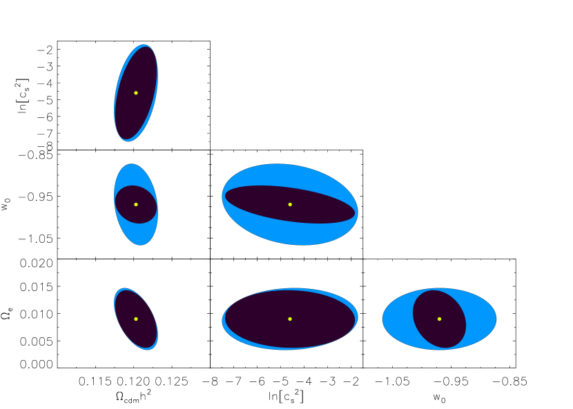
Figure 2: 68% confidence level contours from projected Euclid (black) and DES (light blue) cluster abundances, with projected Planck CMB data, are shown for estimation of pairs of dark cosmology parameters, marginalized over all other parameters. The fiducial parameters are indicated by the yellow dots.

While a fiducial of cold early dark energy can be distinguished clearly from standard early dark energy or no early dark energy, this is not true for a fiducial of standard early dark energy. Table 2 gives the marginalized cosmological parameter estimation for our baseline fiducial sound speed $c_{s}=0.1$, for fiducial $c_{s}=1$, and also when sound speed is fixed to $c_{s}=1$. The sound speed $c_{s}=1$ can be confused with $c_{s}^{2}=1/3$ ($\ln c_{s}^{2}=-1.1$) at $1\sigma$, and we find below that in fact it is essentially unconstrained. This is due to the property discussed earlier that near the extremes of the $c_{s}$ range, not only is the exact value of $c_{s}$ hard to determine, but degeneracies with other parameters come into play. Similar conclusions have been reached recently on constraints projected for weak lensing and galaxy clustering probes 13051942 . To test the robustness of this conclusion we also use $c_{s}^{2}$ rathan than $\ln c_{s}^{2}$ as the parameter.

Case	$\Omega_{c}h^{2}$	$\Omega_{e}$	$w_{0}$	$\ln c_{s}^{2}$	$c_{s}^{2}$
$c_{s}^{2}=0.01$ (fid)	0.0018	0.0035	0.030	$1.82$	$0.018$
$c_{s}^{2}=1$ (fid)	0.0018	0.0057	0.045	$1.42$	$1.43$
$c_{s}^{2}=1$ fixed	0.0018	0.0047	0.042	–	–

Table 2: $1\sigma$ constraints from projected Euclid cluster abundance and future Planck CMB data (full temperature and polarization) on dark energy parameters are compared for different fiducial cases of the sound speed. The last two columns are the errors obtained when the sound speed (squared) parameter is taken to be log or linear, respectively.

Case	$\Omega_{c}h^{2}$	$\Omega_{e}$	$w_{0}$	$\ln c_{s}^{2}$	$c_{s}^{2}$
$c_{s}^{2}=0.01$ (fid)	0.0020	0.0051	0.050	$2.78$	$0.042$
$c_{s}^{2}=1$ (fid)	0.0021	0.0045	0.053	$3.58$	$1.15$
$c_{s}^{2}=1$ fixed	0.0021	0.0046	0.052	–	–

Table 3: As Table 2 but for projected Euclid cluster abundance and current Planck CMB temperature data (including WMAP polarisation data).

The dark energy sound speed constraint arises predominantly from the CMB data. Since a first Planck data release is available, we can compare the constraints using this partial temperature data plus WMAP polarization data wmap9 vs the projected future full temperature plus polarization Planck data. To use the current Planck data, we modify CosmoMC cosmomc and perform a Markov Chain Monte Carlo analysis varying over the standard six cosmological parameters and in addition the cold early dark energy parameters $\Omega_{\rm e}$, $w_{0}$, and $\ln c_{s}^{2}$. These results in combination with projected Euclid cluster data are shown in Table 3. CMB-only constraints, for current data and for projected full Planck data, are shown in Table 4.

Case	$\Omega_{c}h^{2}$	$\Omega_{e}$	$w_{0}$	$\ln c_{s}^{2}$
Current (T + WMAP pol)	0.0030	0.0054	0.350	3.72
Full (TT,TE,EE)	0.0020	0.0039	0.420	1.94

Table 4: Comparison of $1\sigma$ constraints from the CMB-only analysis is shown using the current actual data release (temperature only Planck with WMAP polarisation) vs the projected full Planck temperature and polarization data. In the MCMC analysis using current data the sound speed is only weakly constrained. (Note there is a large difference between the $w_{0}$ best fit value for the MCMC and the fiducial in the projected Fisher analysis).

IV.3 Survey Comparison

Cluster abundance data will become available from DES in the near term, with Euclid data following several years later. Euclid will have a larger sky area, enhanced redshift range, and somewhat lower mass threshold. These will also impact the systematics control. Figure 2 compares the constraints that will be enabled by these cluster surveys when combined with Planck data.

Cluster abundances play an important role in estimating the dark energy equation of state today $w_{0}$, to which the CMB is insensitive, and we find that Euclid will provide significantly improved constraints, by a factor of $\sim 2.5$ better even than DES. The early dark energy sound speed, and energy density, are substantially determined by the CMB data alone.

For cold early dark energy, its density can be determined to 0.3% of the critical density when combining clusters plus CMB, even fitting simultaneously for the sound speed. Cold early dark energy can clearly be distinguished from the canonical case with $c_{s}=1$, if it really is cold, but if it is canonical then cold dark energy cannot be ruled out.

V Conclusions

The halo mass function describing the abundance of massive galaxy clusters is sensitive to properties of both the background expansion and the growth of structure. Since growth involves the expansion history at all earlier times, one might hope to use growth as a probe of the presence of early dark energy, such as appears in many high energy physics theories. However, cluster abundances and other growth measurements have been previously found to have difficulty discriminating early dark energy due to the ability of time varying dark energy to mimic its effects. Here we show that cold early dark energy, where the dark energy perturbation effects are enhanced, can be distinguished by a combination of cluster abundance and CMB data.

The Euclid satellite cluster survey, in conjunction with CMB data, will be able to detect the existence of early dark energy with 0.9% density at the 99% confidence level, and moreover detect that the early dark energy is cold ($c_{s}\lesssim 0.1$) rather than canonical ($c_{s}=1$) at 99% confidence (if it really is cold). Note that early dark energy models obviate the need for the dark energy equation of state today to be significantly different from $w\approx-1$ in order for sound speed to have a reasonable impact. Moreover, many high energy physics models, such as Dirac-Born-Infeld dark energy or various string-inspired models, have specifically cold early dark energy.

Near term cluster surveys such as DES will have sufficient leverage to break degeneracies in CMB data and in combination achieve similar limits on $\Omega_{e}$ and $c_{s}$. The constraints on the present dark energy equation of state will have uncertainties $\sigma(w_{0})\sim 0.06$, improving to $\sim 0.03$ with Euclid.

Interestingly, the complementarity of cluster and CMB data leads to good selfcalibration of the cluster mass systematics, including allowance for redshift evolution in the scatter and bias. The Euclid cluster survey has sufficient information to determine the uncertainty in the scatter, $\sigma(\sigma(\ln M_{0}))$ to 0.033, for example. Further reducing systematics, or tightening the estimation of $\Omega_{c}h^{2}$, would help better determine the sound speed, reducing its fractional uncertainty by almost a factor of 2.

These results offer promising signs for the ability of next generation cluster abundance measurements to probe the nature of early dark energy. Further leverage could come from more precise CMB lensing measurements from ground based polarization experiments, and from crosscorrelation of the CMB with high redshift tracers of the density field (cf. vallinotto ). While lower redshift measurements provide important information on dark energy dynamics, higher redshift measurements of structure growth illuminate the two other important properties of dark energy: its persistence and internal degrees of freedom.

Appendix A Influence of Perturbations on Matter Growth

As discussed in the Introduction, for dark energy perturbations to influence growth of large scale structure one requires the dark energy equation of state to be sufficiently different from $-1$ at a time when there is nonnegligible dark energy density, and a low dark energy sound speed. This led to consideration of the class of cold early dark energy models. If one only includes the expansion effects of the dark energy on the matter growth, and not the impact of the dark energy perturbations, for example through solving the usual second order differential equation for the matter density perturbation $\delta_{m}$ sourced only by itself, then one obtains inaccurate results relative to solving the coupled linear Boltzmann equations, as in for example CAMB.

Here we quantify this deviation in the matter growth from neglecting the dark energy perturbations. Figure 3 shows the growth factor $D(z)$ obtained from solving the usual second order differential equation for growth, $\ddot{D}+2H\dot{D}-4\pi G\rho_{m}(a)D=0$, relative to the growth amplitude of the density power spectrum, $\sqrt{P(z)}$ from CAMB modified for cold early dark energy, all normalized to today. For a canonical cold early dark energy case (such as in the main text) the inaccuracy is of order $(\Omega_{e}/0.02)\%$ at $z=1.5$, scale independent for $k\gtrsim 0.005\,h$/Mpc. Dark energy, early or not, with $c_{s}=1$ has negligible perturbations on these scales, and so negligible deviation. When there is no early dark energy then the deviation is roughly proportional to $(1+w)/(1-3w)$ for constant $w$ with $c_{s}=0$ (see dhl ), and below $0.5\%$ for $w<-0.9$.

Figure 3: Neglect of dark energy perturbations causes deviations in estimation of the matter growth given by $\Delta=[D(z)/D(0)]/\sqrt{P(z)/P(0)}-1$, where the linear matter power spectrum $P$ is calculated including the perturbations and the growth factor $D$ neglects them. The case of cold early dark energy with $\Omega_{e}=0.01$, $c_{s}=0$, $w_{0}=-0.99$ is shown by the solid (nearly identical dotted) curve for wavenumber $k=0.2\,h$/Mpc ($0.005\,h$/Mpc). By contrast, the no early dark energy $w=-0.99$, $c_{s}=0$ case (dashed curve) has negligible perturbations, and the $w=-0.9$, $c_{s}=0$ case (dot-dashed curve) nearly so.

Appendix B Perturbations When Crossing $w=-1$

Given the role that dark energy perturbations can play in structure growth, it is of interest to ensure the perturbations remain well behaved. When $w$ crosses $-1$ (which it does not do for the models considered in the main text), it is not obvious from the Boltzmann evolution equations for the density and velocity perturbations that good behavior is guaranteed. Here we present an analysis demonstrating the conditions under which the crossing does not disrupt the perturbation evolution, including the effect of sound speed behavior. Detailed discussions of the behaviour of dark energy at the $(1+w)=0$ barrier can be found in Hu:2004kh ; Li:2010hm ; Fang:2008sn .

Adopting the conventions of mabert (MB), the metric is

$$g_{00}=-a^{2}(1+2\psi),\ g_{0i}=0,\ g_{ij}=a^{2}(1-2\phi)\delta_{ij}\ ,$$ (7)

and the perturbation equations are

$${k^{2}\over H_{0}^{2}}\phi+3{\cal\bar{H}}^{2}\left(\psi+\phi^{\prime}\right)=-{4\pi Ga^{2}\over H_{0}^{2}}\sum_{i}\rho_{i}\delta_{i}$$ (8)

$$\phi=\psi$$ (9)

$${\cal\bar{H}}\delta^{\prime}=-(1+w)\left(\theta-3{\cal\bar{H}}\phi^{\prime}\right)-3{\cal\bar{H}}\left({\delta P\over\delta\rho}-w\right)\delta$$ (10)

$${\cal\bar{H}}\theta^{\prime}=-{\cal\bar{H}}(1-3w)\theta-{\cal\bar{H}}{w^{\prime}\over 1+w}\theta+{\delta P/\delta\rho\over 1+w}{k^{2}\over H_{0}^{2}}\delta+{k^{2}\over H_{0}^{2}}\psi$$ (11)

$${\cal\bar{H}}\delta^{\prime}_{\rm m}=-\left(\theta_{\rm m}-3{\cal\bar{H}}\phi^{\prime}\right)$$ (12)

$${\cal\bar{H}}\theta^{\prime}_{\rm m}=-{\cal\bar{H}}\theta_{\rm m}+{k^{2}\over H_{0}^{2}}\psi$$ (13)

$$2{\cal\bar{H}}{\cal\bar{H}}^{\prime}=-(1+3w)\left({\cal\bar{H}}^{2}-{\Omega_{\rm m}\over a}-{\Omega_{\rm rad}\over a^{2}}\right)-{\Omega_{\rm m}\over a}-2{\Omega_{\rm rad}\over a^{2}}$$ (14)

$$\rho^{\prime}_{\rm i}=-3(1+w_{\rm i})\rho_{\rm i}$$ (15)

where primes denote differentiation with respect to $N=\ln a$ (or equivalently $x$), $\theta=\theta_{MB}/H_{0}$, $c_{\rm s}^{2}=\delta P/\delta\rho$, and ${\cal\bar{H}}={\cal H}/{\cal H}_{0}$. To solve this system of equations in the vicinity of the time $N_{s}$ when the evolving dark energy equation crosses $w=-1$, we use a power series expansion in $x=N-N_{s}$ and the method of Frobenius.

Specifically, we take

$$w(x)=-1+w_{1}x^{\alpha}+{\cal O}\left(x^{\alpha+1}\right)\ .$$ (16)

Generally we expect $\alpha=1$ but we allow the crossing to be at an inflection point with integer $\alpha>1$. We must also consider the second free function $c_{\rm s}^{2}$, which we parametrize near the crossing as

$$c_{\rm s}^{2}(|x|\ll 1)=c_{0}x^{\beta}\ ,$$ (17)

where $c_{0}$ is a constant and $\beta=0$, $<0$, $>0$ give three distinct cases. We take the ansatz

$$\delta=\sum_{n=0}^{\infty}\delta_{n}x^{n+k_{\delta}}\qquad\theta=\sum_{n=0}^{\infty}\theta_{n}x^{n+k_{\theta}}$$ (18)

$$\delta_{\rm m}=\sum_{n=0}^{\infty}\delta_{\rm m,n}x^{n+k_{\rm m}}\quad\theta_{\rm m}=\sum_{n=0}^{\infty}\theta_{\rm m,n}x^{n+k_{\rm m}}$$ (19)

$$\phi=\sum_{n=0}^{\infty}\phi_{n}x^{n+k_{\phi}}$$ (20)

where $k_{\delta},k_{\theta},k_{\phi}$ are real numbers, determined using the indicial equations of the corresponding series solution. We insert Eqs. (18-20) into Eqs. (8-15).

Before doing so, we calculate $\rho_{\rm i}$ and ${\cal\bar{H}}$ to second order in $x$ using

$${\cal\bar{H}}^{2}={8\pi Ga^{2}\over 3{H}_{0}^{2}}\left(\rho_{\rm m}+\rho_{\rm rad}+\rho_{\rm de}\right)$$ (21)

$$\rho^{\prime}_{\rm m}=-3\rho_{\rm m}$$ (22)

$$\rho^{\prime}_{\rm rad}=-4\rho_{\rm rad}$$ (23)

$$\rho^{\prime}_{\rm de}=-3\left(1+w(N)\right)\rho_{\rm de}\ .$$ (24)

The solution is given by

$$\rho_{\rm m}=\rho_{\rm m,s}\left(1-3x+9x^{2}+{\cal O}(x^{3})\right)$$ (25)

$$\rho_{\rm rad}=\rho_{\rm r,s}\left(1-4x+16x^{2}+{\cal O}(x^{3})\right)$$ (26)

$$\rho_{\rm de}=\rho_{\rm de,s}\left(1-3{w_{1}\over 1+\alpha}x^{\alpha+1}+{\cal O}(x^{\alpha+2})\right)$$ (27)

$${\cal\bar{H}}=\left[{8\pi Ge^{2N_{\rm s}}(\rho_{\rm m,s}+\rho_{\rm r,s}+\rho_{\rm de,s})\over 3{H}_{0}^{2}}\right]^{1/2}$$ (28)

$$\quad\times\left[1-\left({3\rho_{\rm m,s}+4\rho_{\rm r,s}\over 2\rho_{\rm m,s}+2\rho_{\rm r,s}+2\rho_{\rm de,s}}-{1\over 2N_{\rm s}}\right)x\right]+{\cal O}(x^{2})$$

We can now substitute the ansatz for $\delta,\theta$ and the above expansions into the perturbation equations. Assuming the matter perturbations are well behaved during the dark energy crossing implies $k_{\rm m}=0$ and $k_{\phi}=0$. Hence $\delta_{\rm m}$, $\theta_{\rm m}$ and $\phi$ all approach constant values at the crossing $x=0$.

To solve for the remaining variables, we use the expansions for $\theta$ and $\delta$ in Eq. (10). Our approach will be to combine the equations for $\theta$ and $\delta$ by differentiating Eq. (11) and then removing $\delta$ and $\delta^{\prime}$. The resulting second order equation for $\theta$ will yield the indicial equation, the solutions of which will correspond to the leading order behaviour of $\theta$. This can then be used in Eq. (18) to obtain $\delta$. Keeping only the most singular terms, we find the following equation for $k_{\theta}$,

$$k_{\theta}^{2}+(2\alpha-\beta-1)k_{\theta}-\alpha(\beta-\alpha+1)=0\ ,$$ (29)

and $k_{\delta}=0$. This implies the dark energy density perturbation stays constant in an infinitesimal interval around the crossing, but the momentum perturbation may diverge. The two roots of the equation are

$$k_{\theta}=1+\beta-\alpha\quad;\quad k_{\theta}=-\alpha$$ (30)

but the second root always leads to divergence. The first root gives stable perturbations for $\beta\geq\alpha-1$. If $\beta<0$, i.e. the sound speed diverges at the crossing, then the momentum does as well for all $\alpha$.

The key criterion

$$\beta\geq\alpha-1$$ (31)

can be seen heuristically from the $\theta^{\prime}$ equation. Terms on the right hand side can diverge no more severely than $x^{-1}$ in order that the integration over $x$ to get $\theta$ gives a bounded $\theta$. For the term involving $w^{\prime}/(1+w)\sim x^{-1}$ this is fulfilled for all $\alpha$, but the sound speed term gives $x^{\beta}/x^{\alpha}=x^{\beta-\alpha}$ so we require $\beta-\alpha\geq-1$, precisely the criterion above.

The next to leading order behaviour is dependent upon the values of $\alpha,\beta$. If we concentrate on the case $(\alpha,\beta)=(1,0)$, then we find

$$\delta_{1}=-\frac{w_{1}}{{\cal\bar{H}}_{\rm s}}\theta_{0}-3(1+c_{0})\delta_{0}$$ (32)

$$\theta_{1}=-4\theta_{0}+\frac{c_{0}}{w_{1}{\cal\bar{H}}_{\rm s}}\frac{k^{2}}{{H}_{0}^{2}}\delta_{0}\ .$$ (33)

The zeroth order coefficients $\delta_{0}$ and $\theta_{0}$ are determined by the two initial conditions required for the two first order equations. The divergent second root $\theta\sim x^{-\alpha}$ can be removed by setting the initial condition such that $\theta_{0}=0$. The dark energy perturbations in the vicinity of the crossing are therefore well behaved for this case, with

$$\delta=\delta_{0}\left(1-3(1+c_{0})x+{\cal O}(x^{2})\right)$$ (34)

$$\theta=\delta_{0}\left(\frac{c_{0}}{w_{1}{\cal\bar{H}}_{\rm s}}\frac{k^{2}}{{H}_{0}^{2}}+{\cal O}(x)\right)\ .$$ (35)

Of course, in numerical studies it is not possible to evade the divergent root of $\theta$ by choosing initial conditions appropriately, and so one must resort to other means Hu:2004kh ; Li:2010hm . The underlying physics of the singular solution at the crossing is well understood Fang:2008sn .

References

- (1) N. Suzuki et al., ApJ 746, 85 (2012) [arXiv:1105.3470]
- (2) C. Blake et al., MNRAS 425, 405 (2012) [arXiv:1204.3674]
- (3) B.A. Reid et al., MNRAS 426, 2719 (2012) [arXiv:1203.6641]
- (4) J. Weller, A. Lewis, MNRAS, 346, 987 (2003)
- (5) R. Bean, O. Doré, PRD, 69, 083503 (2004)
- (6) R. de Putter, O. Zahn, E.V. Linder, Phys. Rev. D 79, 065033 (2009) [arXiv:0901.0916]
- (7) R. de Putter, D. Huterer, E.V. Linder, Phys. Rev. D 81, 103513 (2010) [arXiv:1002.1311]
- (8) E. Calabrese, R. de Putter, D. Huterer, E.V. Linder, A. Melchiorri, Phys. Rev. D 83, 023011 (2011) [arXiv:1010.5612]
- (9) E. Calabrese, D. Huterer, E.V. Linder, A. Melchiorri, L. Pagano, Phys. Rev. D 83, 123504 (2011) [arXiv:1103.4132]
- (10) S. Joudaki & M. Kaplinghat, Phys. Rev. D 86, 023526 (2012) [arXiv:1106.0299]
- (11) C.L. Reichardt, R. de Putter, O. Zahn, Z. Hou, ApJ 749, L9 (2012) [arXiv:1110.5328]
- (12) C. Wetterich, Phys. Lett. B 594, 17 (2004) [arXiv:astro-ph/0403289]
- (13) M. Doran & G. Robbers, JCAP 0606, 026 (2006) [arXiv:astro-ph/0601544]
- (14) M.J. Francis, G.F. Lewis, E.V. Linder, MNRAS 394, 605 (2008) [arXiv:0808.2840]
- (15) M. Grossi & V. Springel, MNRAS 394, 1559 (2009) [arXiv:0809.3404]
- (16) M.J. Francis, G.F. Lewis, E.V. Linder, MNRAS Letters 393, L31 (2008) [arXiv:0810.0039]
- (17) U. Alam, Z. Lukić, S. Bhattacharya, ApJ 727, 87 (2011) [arXiv:1004.0437]
- (18) D. Sapone, M. Kunz, L. Amendola, Phys. Rev. D 82, 103535 (2010) [arXiv:1007.2188]
- (19) E.V. Linder & A. Jenkins, MNRAS 346, 573 (2003) [arXiv:astro-ph/0305286]
- (20) G. Ballesteros & J. Lesgourgues, JCAP 1010, 014 (2010) [arXiv:1004.5509]
- (21) H. Oyaizu, Phys. Rev. D 78, 123523 (2008) [arXiv:0807.2449]
- (22) B. Li, G.-B. Zhao, R. Teyssier, K. Koyama, JCAP 01, 051 (2012) [arXiv:1110.1379]
- (23) E. Puchwein, M. Baldi, V. Springel, arXiv:1305.2418
- (24) J.L. Tinker, A.V. Kravtsov, A. Klypin, K. Abazajian, M.S. Warren, G. Yepes, S. Gottlober, D.E. Holz, ApJ 688, 709 (2008) [arXiv:0803.2706]
- (25) A. Lewis, A. Challinor, & A. Lasenby, ApJ 538, 473 (2000) [arXiv:astro-ph/9911177]; http://camb.info
- (26) A. Jenkins, C.S. Frenk, S.D.M. White, J.M. Colberg, S. Cole, A.E. Evrard, H.M.P. Couchman, N. Yoshida, MNRAS 321, 372 (2001) [arXiv:astro-ph/0005260]
- (27) R.K. Sheth & G. Tormen, MNRAS 308, 119 (1999) [arXiv:astro-ph/9901122]
- (28) M.S. Warren, K. Abazajian, D.E. Holz, L. Teodoro, ApJ 646, 881 (2006) [arXiv:astro-ph/0506395]
- (29) R. C. Batista and F. Pace, arXiv:1303.0414 [astro-ph.CO].
- (30) E.V. Linder & G. Robbers, JCAP 0806, 004 (2008) [arXiv:0803.2877]
- (31) R. Laureijs et al, ESA/SRE(2011)12 [arXiv:1110.3193]; http://www.euclid-ec.org
- (32) http://www.darkenergysurvey.org
- (33) C. Cunha, D. Huterer and J. A. Frieman, Phys. Rev. D 80 (2009) 063532 [arXiv:0904.1589 [astro-ph.CO]].
- (34) C. E. Cunha and A. E. Evrard, Phys. Rev. D 81 (2010) 083509 [arXiv:0908.0526 [astro-ph.CO]].
- (35) M. Lima and W. Hu, Phys. Rev. D 72 (2005) 043006 [astro-ph/0503363].
- (36) E. S. Rykoff, B. P. Koester, E. Rozo, J. Annis, A. E. Evrard, S. M. Hansen, J. Hao and D. E. Johnston et al., Astrophys. J. 746 (2012) 178 [arXiv:1104.2089 [astro-ph.CO]].
- (37) A. Biviano, private communication and for the Euclid Red Book
- (38) E. Rozo, private communication.
- (39) P. A. R. Ade et al. [Planck Collaboration], arXiv:1303.5076 [astro-ph.CO].
- (40) P.A.R. Ade et al, A&A, 536, A1 (2011); http://planck.esa.int
- (41) D. Sapone, E. Majerotto, M. Kunz, B. Garilli, arXiv:1305.1942
- (42) C.L. Bennett et al, arXiv:1212.5225
-
(43)
A. Lewis & S. Bridle, Phys. Rev. D 66, 103511 (2002)
[arXiv:astro-ph/0205436]
http://cosmologist.info/cosmomc - (44) A. Vallinotto, arXiv:1304.3474
- (45) W. Hu, Phys. Rev. D 71 (2005) 047301 [astro-ph/0410680].
- (46) M. Li, Y. Cai, H. Li, R. Brandenberger and X. Zhang, Phys. Lett. B 702 (2011) 5 [arXiv:1008.1684 [astro-ph.CO]].
- (47) W. Fang, W. Hu and A. Lewis, Phys. Rev. D 78 (2008) 087303 [arXiv:0808.3125 [astro-ph]].
- (48) C-P. Ma & E. Bertschinger, ApJ 455, 7 (1995) [arXiv:astro-ph/9506072]