Applications of Temporal Graph Metrics to Real-World Networks
Abstract
Real world networks exhibit rich temporal information: friends are added and removed over time in online social networks; the seasons dictate the predator-prey relationship in food webs; and the propagation of a virus depends on the network of human contacts throughout the day. Recent studies have demonstrated that static network analysis is perhaps unsuitable in the study of real world network since static paths ignore time order, which, in turn, results in static shortest paths overestimating available links and underestimating their true corresponding lengths. Temporal extensions to centrality and efficiency metrics based on temporal shortest paths have also been proposed. Firstly, we analyse the roles of key individuals of a corporate network ranked according to temporal centrality within the context of a bankruptcy scandal; secondly, we present how such temporal metrics can be used to study the robustness of temporal networks in presence of random errors and intelligent attacks; thirdly, we study containment schemes for mobile phone malware which can spread via short range radio, similar to biological viruses; finally, we study how the temporal network structure of human interactions can be exploited to effectively immunise human populations. Through these applications we demonstrate that temporal metrics provide a more accurate and effective analysis of real-world networks compared to their static counterparts.
1 Introduction
Temporal graph metrics TMML09:temporal ; tang_analysing_2010 represent a powerful tool for the analysis of real-world dynamic networks, especially with respect to the aspects for which time plays a fundamental role, such as in the case of spreading of a piece of information or a disease. Indeed, existing metrics are not able to characterise the temporal structure of dynamic networks, for example in terms of centrality of nodes over time. For these reasons, new metrics have been introduced, such as temporal centrality, in order to capture the essential characteristics of time-varying graphs. A detailed description of the metrics used in this chapter can be found in NTMMRL12:graphs .
In this chapter we will discuss a series of possible applications of temporal graph metrics to the analysis of real-world time-varying networks. This chapter is structured as follows. We will cover our work in this area and, finally, we will discuss contributions in this fields by other researchers and potential future applications, in particular in the area of the modelling of epidemic spreading.
More specifically, in Section 2 we analyse the roles of key individuals according to temporal centrality within the context of the Enron scandal tang_analysing_2010 . In Section we study how such temporal metrics can used to study the robustness of temporal networks in presence of random errors and intelligent attacks SLMBZ12:evaluating . Then, Section 4 we present a containment scheme for mobile phone malware which can spread via short range radio transmission TMML11:exploiting ; THMM12:STOP . Finally, in Section 5 we discuss existing and potential applications to human epidemiology, outlining some research directions in these areas.
2 Corporate Networks
2.1 Overview
The Enron Energy Corporation started as a traditional gas and electrical utility supplier; however, in the late 1990s their main money making business came from trading energy on the global stock markets elkind_smartest_2004 . In December 2001, the Enron Energy Corporation filed for bankruptcy after it was uncovered that fraudulent accounting tricks were used to hide billions of dollars in debt _addressing2000-2001_2008 . This led to the eventual conviction of several current and former Enron executives laurel_brubaker_calkins_enron_2004 ; lauren_johnston_former_2004 . The investigation also brought to light the reliance of the company on traders to bring in profits using aggressive tactics culminating in intentional blackouts in California in Summer 2001. With both control over electricity plants and the ability to sell electricity over the energy markets, Enron traders artificially raised the price of electricity by shutting down power plants serving the State of California and profiting by selling electricity back at a premium cali_enron_2004 .
During the investigation into the Enron accounting scandal, telephone calls, documents and emails were subpoenaed by the U.S. government and as such the email records of 151 user mailboxes were part of the public record consisting of approximately 250,000 emails sent and received during the period between May 1999 to June 2002 (1137 days), leading up to the bankruptcy filing. None of the emails were anonymised and so they provide unique semantic information of the owner of each mailbox.
2.2 Temporal Graph Construction
In our analysis, we use the dataset prepared by Shetty & Adibi shetty_discovering_2005 . Since we do not have a complete picture of the interactions of users outside of the subpoenaed mailboxes we concentrate on email exchanges between the core 151 users only. Taking this email dataset, we process the complete temporal graph from 1999 to 2002 with undirected links, using windows of size =24 hours and horizon =1. If an email was exchanged between two individuals in a temporal window, a link between the two nodes representing those individuals will be added to the graph representing the temporal snapshot for that time.
2.3 Semantic Value of Temporal Centrality
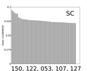
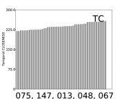
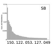
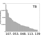
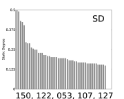
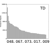
Figure 1 plots the static and temporal centrality rankings of employees calculated using closeness and betweenness. Examining the static centralities (left column) we note that there is little difference between the top five employees using static closeness or betweenness. Also plotting the static degree centrality of each node111The static degree centrality is defined as the number of edges connected to a node , normalised by the total possible neighbour nodes wasserman_social_1994 , we notice similar rankings suggesting that static analysis only favours employees who interacted with the most number of other people. Temporal closeness and temporal betweenness yield different rankings amongst the top five and the calculated Kendall-tau correlation coefficientkendall_new_1938 (Table 2) confirm that static-to-static metrics are strongly correlated (). Also note that there is low correlation () between temporal metrics and static degree demonstrating that temporal analysis is not dependent on the number of people an individual interacts with.
Cross referencing the top two employee identifiers with their position within the organisation (Table 1) we identify a secretary (150) and managing director (122) as central nodes for both static closeness and betweenness; however, both temporal closeness and betweenness consistently selected employees in trading roles (053, 075, 107, 147). A secretary and a managing director are certainly important for information dissemination and central to many communication channels, as detected by static measures. However, instead the top trading executives are exclusively favoured by temporal analysis.
To show that temporal analysis does not simply uncover nodes with the most interactions with other people, we also plot the temporal degree (TD) calculated as the total number of emails sent and received by each node . Since there is a low correlation () with temporal closeness and betweenness this shows that temporal analysis is not dependent on the number of emails sent and received by each individual.
| ID | Role | Notes |
|---|---|---|
| 9 | (Unknown) | |
| 13 | Legal | Senior Legal Specialist |
| 17 | Manager | |
| 48 | Executive | |
| 53 | Trader | |
| 54 | President | Former Head of Trading |
| 67 | Vice President | Enron Wholesale Services |
| 73 | Trader | |
| 75 | Director of Trading | |
| 107 | Trader | Head of Online Trading |
| 122 | Managing Director | |
| 127 | Chairman & CEO | |
| 139 | Director | |
| 147 | Trader | |
| 150 | Secretary | Assistant to Greg Whalley |
| SB | SC | SD | TB | TC | TD | |
|---|---|---|---|---|---|---|
| SB | 1.00 | 0.57 | 0.69 | 0.41 | 0.24 | 0.43 |
| SC | - | 1.00 | 0.70 | 0.36 | 0.22 | 0.31 |
| SD | - | - | 1.00 | 0.39 | 0.28 | 0.48 |
| TB | - | - | - | 1.00 | 0.43 | 0.34 |
| TC | - | - | - | - | 1.00 | 0.40 |
| TD | - | - | - | - | - | 1.00 |
2.4 Effectiveness of Central Nodes on Dynamic Processes
Trace-driven Simulation Setup
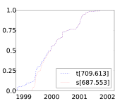
To evaluate the role and the centrality of the employees identified by temporal and static analysis, we consider two dynamic processes. First, we simulate a simple information dissemination process over the temporal graph constructed from the Enron traces. The process is simulated as follows. We select the top nodes from the ranking based on temporal closeness centrality. We place an identical message into their (infinite) buffers. We refer to any node that has received a copy of this message as reached. We then replay the contact trace through time and as reached nodes make contact with an unreached node , the message is replicated into the buffer of node . We assume that messages are transferred instantaneously and only the first neighbour in a time window can be reached. We then repeat this for static closeness centrality and plot the dissemination ratio across time for both.
Second, to model the role of individuals as part of an information mediation process, we borrow concepts from the more commonly known epidemic immunisation process where the dissemination ratio of a contagion spreading throughout a static network is measured before and after certain nodes are immunised against the contagion barrat_dynamical_2008 . This is analogous to measuring the spread of information (the contagion) before and after important individuals are removed from the network (such as going on holiday or being discharged) since our conjecture is that removing mediators will impact the network communication efficiency greatly.
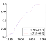
In the trace-driven simulation, instead of a single message spreading within the organisation, we seed all employees with a different message that needs to be delivered to all other employees. This models multiple channels of communication. In order to derive a baseline performance, we start by calculating the dissemination ratio when no nodes are removed. We then remove the top individuals identified by temporal betweenness and rerun the information spreading process. Nodes which are removed cannot receive or pass on messages. We then repeat the same process for comparison using static betweenness centrality for the ranking.
Evaluating Information Dissemination & Mediation
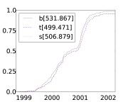
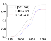
We present plots using for information dissemination (Figure 2) and information mediation (Figure 3). As we can see the different pairs of traders identified by temporal analysis are better than the arbitrary nodes selected by static analysis for both disseminating information through the organisation and acting as mediators between communication channels. In the information dissemination case, although the final dissemination is the same across the long period of time, the two traders selected by temporal analysis disseminate information quicker. Only after increasing to 10 nodes the static analysis presents similar results. In the information mediation case, the final dissemination ratios for both temporal and static centrality nodes slightly decreases by removing the nodes but are comparable. However, removing the two traders gives an overall more prolonged drop in message dissemination. In the case of the removal of 10 nodes, the individuals identified by means of the temporal metrics slow the dissemination process further compared to static ones.
2.5 Summary of the Findings
This study has demonstrated the advantages of using temporal network analysis over traditional static, aggregated graphs. Although centrality rankings are quantitative measures of node importance, their physical meaning is very much qualitative. For this reason, we have shown that temporal centrality provides a more accurate identification of key people in a corporate social network where each persons role is known. Taking a second perspective, we demonstrate that temporal centrality can identify nodes which can spread and mediate information, better than static analysis. This demonstrates the importance of temporal information for applications which are applied to real networks.
3 Network Robustness
3.1 Overview
The study of real-world communication systems by means of complex network models has provided insightful results and has vastly expanded our knowledge on how single entities create connections and how these connections are used for communication or, more generally, interaction BOCCALETTI2006 . In particular, technological networks such as the Internet and the World Wide Web have been under scrutiny in terms of structure and dynamic behavior Huberman99 ; Faloutsos1999 . More recently, with the widespread adoption of mobile and opportunistic networks, it has become important to develop new analytical tools to keep into account network dynamics over time Kostakos2009 ; Kempe2000 and how this affects phenomena such as information propagation CE07:persistence ; Chaintreau_CHCDGS07:Impact .
At the same time, the problem of understanding whether real systems can sustain substantial damage and still maintain acceptable performance has been extensively addressed albert_error_2000 ; callaway2000 . Various measures of network robustness have been defined and investigated for several classes of networks, evaluating how different system can be more or less resilient against random errors or targeted attacks thanks to their underlying structural properties holme2002 ; crucitti2004 .
Nonetheless, it is still unclear how to approach the study of robustness of networks by taking into account their time-varying nature: by adopting a static representation of a temporal network, important features which impact the actual performance might be missed. Thus, it becomes important to develop a robustness metric which takes into account the temporal dimension and gives insights on how a mobile network is affected by damage or change. Particularly, the fact that links are not always active means that information spreading can be delayed or even stopped and that relative ordering in time of connection events may affect the creation of temporal paths in mobile networks.
Our main goal is to design a novel framework for the analysis of robustness in time-varying networks. We adopt temporal network metrics TMML09:temporal to quantify network performance and define a measure of robustness against generic network damages. At first, we study its performance on random network models to understand its properties; then we apply our method to study a real mobile network, describing how temporal robustness gives a more accurate evaluation of system resilience than static approaches.
3.2 A Framework to Evaluate Robustness of Temporal Networks
The study of robustness of complex networks has mainly focused on describing how a given performance metric of the network is affected when nodes are removed according to a certain rule. The underlying assumption is that the absence or malfunctioning of some nodes will cause the removal of their edges and, thus, some paths will become longer, increasing the distances between the remaining nodes, or completely disappear, resulting in the loss of connectivity in the whole system. In this work we will study the problem of defining and analyzing robustness in evolving networks: as a consequence, we need to use a performance metric which includes the temporal dimension in its definition. We choose to adopt temporal efficiency as the performance metric. We then consider random and independent failures for every node and we evaluate how the system tolerates increasing level of malfunctioning nodes.
Since a temporal graph is continuously evolving, we can evaluate how temporal efficiency changes over time by considering a value and evaluating as the relative temporal efficiency of the temporal graph in the time window . The effect of is to effectively impose an upper bound on the temporal distances, as all paths longer than simply do not exist. As a consequence, should be chosen so that any communication whose delay is longer than itself can be ignored.
Given a temporal graph , we define a damage as any structural modification on it and we define as the graph resulting by the effect of the damage on . A damage may be the deactivation of some nodes or the removal of some edges at a particular time . Because of damage , some temporal shortest paths will be longer or will not exist any more, thus, we expect that the temporal efficiency will eventually reach a new steady value . It is important to evaluate the new value of the temporal efficiency on a new temporal graph which still contains the deactivated nodes, in order to obtain a decrease in efficiency. Otherwise, we might obtain a smaller temporal graph which is more efficient than the original graph, although it has lost much of its structure. Hence, we do not consider highly dynamic systems where nodes can be constantly added or removed. Instead, we focus on evaluating the service degradation in a more controlled environment where only a number of existing nodes could fail.
We define the loss in efficiency caused by the damage on the temporal graph as . Finally, we define the temporal robustness of the temporal graph against the damage as
| (1) |
This value is normalized between 0 and 1 and it measures the relative loss of efficiency caused by the damage: if the damage does not impact the efficiency of the graph () then its robustness is 1, while if the damage destroys the efficiency of the graph () the robustness drops to 0. Temporal efficiency is a particularly suitable metric to study temporal network robustness as it denotes both longer temporal paths and the lack of paths among temporally disconnected nodes at the same time. Nonetheless, other metrics have been used to assess robustness in static systems: for instance, there could be scenarios where fast communication with small delays can be more important than global connectivity, thus other measures can be adopted. Provided that these measures can be extended to the temporal case, they can be easily integrated in our framework.
3.3 Robustness of Random Temporal Networks
In this section, we present a numerical analysis of temporal robustness for different classes of random temporal networks: an Erdős-Rényi temporal model, a Markovian temporal model and mobility-based temporal model.
Random Temporal Network Models
An Erdős-Rényi (ER) random graph with nodes and parameter is created by independently including each possible edge in the graph with probability and it is denoted as ErdRen60 . We generalize this model to the temporal case by creating a sequence of ER random graphs and we denote the resulting temporal graph as .
The temporal ER network model does not provide temporal correlations between consecutive graphs in the sequence. We thus consider a model where link evolution is described by a Markov process, thus enabling memory effects in network dynamics. We consider a complete graph with nodes. At every discrete timestep each link may or may not be present: a temporal graph is created where the existence of each link evolves according to a 2-state discrete Markov process. We denote with the probability that a link present at time will be removed at time and with the probability that a link which is not present at time will be added at time . The steady probability of link presence then is : as a consequence, each observation of the temporal graph appears as an ER random graph with each edge present with probability .
We also create a random model of a temporal network by using mobility models. In this case we are introducing topological constraints: a key difference with the previous temporal models is that each node is not equally likely to connect with all the other nodes, due to the effect of spatial distance. We consider nodes moving in a square area x meters and we define a communication range : at every time step, we create a graph where nodes are connected if their Euclidean distance is shorter than . Thus, we change the probability of link presence by varying the communication range. Then, a temporal graph can be defined as the sequence of graphs extracted at each time step while the nodes move. We investigate two different mobility models that are implemented using the Universal Mobility Model Framework ummf : Random Waypoint Model (RWP) and Random Waypoint Group Model (RWPG). In RWP each node selects uniformly at random a location towards which it moves with speed uniformly distributed in a fixed range mph. As the node reaches its destination, it waits for a randomly distributed time in seconds and repeats the above steps until the end of the simulation.
In RWPG nodes are divided into two classes: there are group leaders and group followers. Every group followers has its own leader so that the nodes are divided into equally-sized groups. Each group leader selects a random target and moves towards it, according to the RWP mobility model. Group members do not select any target; instead, they follow their group leader according to the pursuit force ummf which is set to give a group span of 200 meters.
Numerical Evaluation
We numerically evaluate temporal efficiency over time, adopting a time window of , for a graph with nodes: after an initial phase, the random temporal graph reaches an equilibrium state and we compute the steady value of temporal efficiency. We run each simulation for steps and we compute the average value of temporal efficiency over the last steps. All results have been averaged over 100 different runs. We evaluated numerically temporal robustness by deactivating each node independently with increasing probability . We measure temporal efficiency before and after the failure, when the network reaches a new equilibrium state.
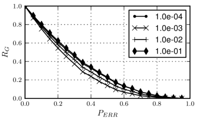

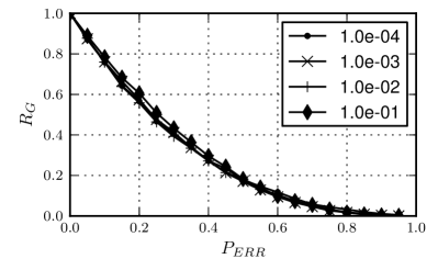
As reported in Figure 4, the temporal ER model fails smoothly as we increase the fraction of removed nodes, without any sudden disruption for any value of . This is a main difference with respect to what happens in the static case: for a static ER random graph there may exist a critical value of which causes a breakdown of the network in several disconnected components albert_error_2000 . This is not true for temporal robustness, as new paths can still appear after the damage as the network rearranges its connections. Time provides more redundancy and, hence, more resilience. Moreover, we also note that temporal robustness does not depend on system size: since it is normalized with respect to the value of temporal efficiency before the damage, it depends only on the relative drop in efficiency, not on absolute values.
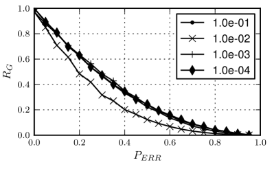
As shown in Figure 5(a), temporal robustness is affected by probability of error in the same way as in the temporal ER model: the system fails gradually as more nodes are removed. However, for intermediate values of robustness has lower values. At the same time, high and low values of provide the same robustness, even if the absolute value of temporal efficiency can be very different, thanks to the normalization of temporal robustness.
In the case of mobility-based temporal networks, reported in Figure 5(b), both RWP and RWPG exhibit a similar behavior: again, the network loses efficiency in a smooth way and temporal robustness is not affected by in this case as the spatial characteristics of the network are mainly affecting the resulting robustness.
3.4 Case Study: Cabspotting
We have seen that temporal networks do not exhibit sudden breakdowns when nodes are being removed and that various temporal network models exhibit analogies in their resilience. We now shift our attention to real time-varying networks: our aim is to understand whether temporal robustness gives us more information than static robustness in a real case and to investigate whether random models can offer a good approximation to real networks.
Dataset
This case study is based on Cabspotting, a publicly available dataset of mobility traces: the Cabspotting project tracked taxi cabs in San Francisco traveling through all the Bay Area for about two years with the aim of gathering data about city life cabspotting . The vehicles were equipped with GPS sensors and every device was periodically updating its position and uploading it to a central server to be stored, along with the timestamp of the record. Thus, it is possible to reconstruct each taxi’s trajectory over space. For pictorial representations of the dataset, please refer to the project website cabspottingproject .
We have selected an area of about 20 km x 20 km around the city of San Francisco and we have extracted 24 consecutive hours of mobility traces, corresponding to Wednesday, 21 May 2008. After this, we have generated an artificial contact trace by defining a communication range of 200 m for the vehicles, which roughly corresponds to WiFi connectivity range in similar scenarios Chaintreau2009 : whenever two cars are within this distance they can communicate to each other. Time granularity is in seconds, so we have a sequence of 86,400 graphs with 488 nodes and more than 350,000 contacts among them. The average contact duration is about 2 minutes while the average inter-contact time is more than 2.5 hours.
Analysis
We study the reaction of the Cabspotting temporal network to random failures and compare it to our findings on random models. We adopt numerical simulation, but since the temporal dynamics of this network is not stationary, we can not compare the temporal efficiency before and after a certain error, because the two temporal window will likely have already different properties. Instead, we fail nodes according to at the very first time step of the temporal sequence of graphs: in this way, we can compare the average temporal efficiency over all the time for the original network and for the damaged one. We adopt a value of , which allows us to consider temporal paths up to 1 hour, even if such longer paths can not contribute much to temporal efficiency.
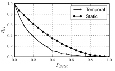
The first comparison that we show in Figure 6 is between static robustness and temporal robustness for the Cabspotting temporal network. In this case static robustness is computed on the static graph obtained by aggregating all the contacts in the trace and adopting static global efficiency as performance measure. Since the resulting static graph contains more than 100,000 edges it is clearly an overestimation of the communication properties of the real system, as not all these links are continuously available over time and some paths can not be used due to temporal ordering constraints. Indeed, static robustness appears much larger than the temporal counterparts: only temporal robustness is able to capture the realistic communication capabilities of the system and how they are affected by random failures.
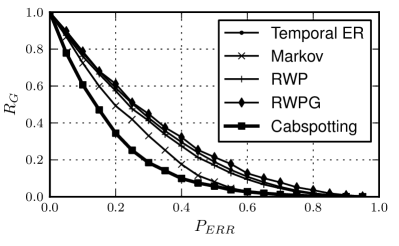
Then, we attempt to understand if the various random temporal network models we have studied can be used to approximate the robustness properties of the real scenario. For each model, we compute the temporal robustness as a function of for a network with the same number of nodes and the same measured in the Cabspotting temporal network (about ), using the same simulation parameters as in the real scenario. As reported in Figure 6, all temporal networks present the same trend in network robustness, albeit random models have higher values of temporal robustness than the real network. Interestingly, the closest match is the Markov-based temporal model, while the mobility-based models are closer to the ER model than to the Cabspotting network, even if this is actually a mobility-based contact network. However, the assumptions used in mobility models require homogeneity of space and absolute freedom to move continuously and independently in a boundless area, while in reality taxis are usually constrained to move on streets and bridges and they often move together along the same direction or stop together in a particular place to wait for customers (i.e., airport or stations). The Markov model, instead, introduces the type of time correlations that appear to better mimic the real scenario. In fact, the most important aspect that needs to be captured is time ordering of events: in random mobility models connections do not follow particular time patterns, whereas real traces do (rush hour, working hours, human sleeping cycles). Only temporal robustness can take into account these unique characteristics.
3.5 Summary of the Findings
These two results provide evidence that temporal robustness is a more accurate measure to be used on mobile networks instead of standard static approaches. Therefore, when testing protocols and applications to be deployed in mobile networks, a temporal study is more meaningful and should not be substituted by a static approximation.
4 Mobile Malware
4.1 Overview
Smartphones are not only ubiquitous, but also an essential part of life for many people who carry such devices through their daily routine. It comes at no surprise then that recent studies have shown that the mobility of such devices mimic that of their owners’ schedule eagle_reality_2006 ; wang_understandingspreading_2009 . This fact constitutes an opportunity for devising efficient protocols and applications, but it also represents an increasing security risk: as with biological viruses that can spread from person to person, mobile phone viruses can also leverage the same social contact patterns to propagate via short-range wireless radio such as Bluetooth and WiFi. For example, when security researchers downloaded Cabir cabir – the first proof-of-concept piece of mobile malware – for analysis, they soon discovered the full risk potential of the mobile worm as it broke loose, replicating from the test device to external mobile phones. This event prompted the need for specially radio shielded rooms to securely test such malicious code f-secure_2005 .
Unlike desktop computers mobile malware can spread through both short-range radio (i.e., Bluetooth and WiFi) and long-range communication (SMS, MMS and email) leavitt_mobile_2005 . Long-range malicious traffic can potentially be contained by the network operator by scanning every message against a database of known malware or spam van_ruitenbeek_quantifyingeffectiveness_2007 , however, short-range propagation might fall under the radar of centralised service providers: effective schemes to defend against short-range mobile malware spreading are necessary. In addition, while a global patching of the devices through cellular connectivity is the natural solution and is in theory possible, in practice, due to associated costs and resource consumption, this is not ideal. For example, there are potential constraints with respect to the cellular network capacity and server bandwidth (with respect to the latter, similar issues have also investigated for software updates distribution in the Internet, see for example GKC06:planet ).
4.2 Temporal Centrality Metrics for Malware
Being highly correlated with human contacts, understanding how such malware propagates requires an accurate analysis of the underlying time-varying network of contacts amongst individuals. State-of-the-art solutions on mobile malware containment have ignored two important temporal properties: firstly, the time order, frequency and duration of contacts; and secondly, the time of day a malicious message starts to spread and the delay of a patch zhu_social_2009 ; zyba_defending_2009 . Instead, we argue that the temporal dimension is of key importance in devising effective solutions to this problem.
With this in mind, the focus of this study is to investigate the effectiveness of two containment strategies based on targetting key nodes, taking into account these temporal characteristics. We firstly investigate a traditional strategy, inspired by studies on error and attack tolerance of networks albert_error_2000 , exploiting static and a time-aware enhanced version of betweenness centrality which provide the best measure of how nodes that mediate or bridge the most communication flows. According to this strategy the nodes that act as mediators are patched to block the path of a malicious message. However, due to temporal clustering and alternative temporal paths, in most cases, such strategies merely slow the malware and does not stop it. In other words, a scheme based solely on immunisation of key nodes is not sufficient, instead quick spreading of the patch is necessary for most networks. We propose a solution based on local spreading of patches through Bluetooth, i.e., exploiting the same mechanism used by the malware itself. The key issue in this approach is to select the right nodes as starting points of the patching process. using temporal closeness centrality which ranks nodes by the speed at which they can disseminate a message to all other nodes in the network. We show that this strategy can reduce the cellular network resource consumption and associated costs, achieving at the same time a complete containment of the malware in a limited amount of time.
4.3 Evaluation
| CAMBRIDGE | INFOCOM | MIT | |
|---|---|---|---|
| N | 18 | 78 | 100 |
| Duration | 10 Days | 5 days | 280 days |
| Contacts (avg. per day) | 1927 | 25796 | 231 |
| Scanning Rate | 30 sec | 2 min | 5 min |
4.4 Simulation Setup
To evaluate the time-aware mobile malware containment schemes, three traces of real mobile device contacts carried by humans are used: Bluetooth traces of researchers at the University of Cambridge, Computer Laboratory, as part of an emotion sensing experiment rachuri_emotionsense_mobile_2010 ; Bluetooth traces of participants at the 2006 INFOCOM conference cambridge-haggle-2009-05-29 ; and campus Bluetooth traces of students and staff at MIT eagle_reality_2006 . We shall refer to these as CAMBRIDGE, INFOCOM, MIT, respectively. Table 3 describes the characteristics of each set of traces. All three datasets were constructed from mobile device co-location where participants were given Bluetooth enabled mobile devices to carry around. When two devices come into communication range of the Bluetooth radio, the device logs the colocation with the other device. For the CAMBRIDGE dataset, all 10 days are used as part of the evaluation. For the INFOCOM dataset, since devices were not handed out to participants until late afternoon during the first day, only the last 4 days are used. For the MIT dataset, we show results for the first two weeks of the Fall semester representing a typical fortnight of activity.
The top devices are chosen according to the calculated temporal betweenness or temporal closeness centrality ranking from the temporal graph , where is set to the finest window granularity, corresponding to the scanning rate of the devices in each dataset (for example, 30 second windows for CAMBRIDGE); and is set to 1, since higher values of lead to similar performance of the containment schemes. The nodes that are initially infected with malicious messages are chosen uniformly randomly. The results are obtained by averaging over 100 runs for each . The static centralities from the static aggregated graph over the time interval are also calculated for comparison.
Our evaluation is based on the following assumptions: firstly, when a node receives a patch message, it is immunised for the rest of the simulation (i.e., we assume that the malware does not mutate over time); secondly, there is always a successful file transfer between devices (errors in transmission can be taken into consideration in the assessment of the contention scheme without changing significantly the results of our work, assuming random transmission failures); thirdly, an attacker chooses nodes at random; and finally, we have no knowledge of which devices are compromised (otherwise the best scheme is to patch those devices immediately).
4.5 Non-Effectiveness of Betweenness based Patching
Starting from the results of the analysis of the effects time of day has on message spreading, we now evaluate the best case scenario for the containment scheme based on patching nodes (without spreading the patch) and we show that this is highly inefficient since it requires a very large number of nodes to be patched via the cellular network to be effective.
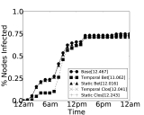
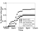
Using Day 4 of the INFOCOM trace for this example, a piece of malware is started at the beginning of the day (=12am) and the device(s) are patched at the same time (=12am). This is the best case scenario for two reasons: first, the temporal graph in the morning is characterised by low temporal efficiency since there are very few contacts, therefore, the malware spreads slowly ; secondly, devices that are immunised immediately have the best chance of blocking malware spreading routes.
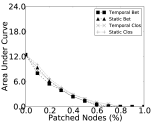
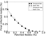
Figure 7 shows the ratio of compromised devices across time when the top 1 (top left panel) and top 10 (top right panel) devices are patched after being selected using betweenness and closeness. As we can see, temporal betweenness initially perform better than static betweenness and both temporal and static closeness (quantified by the difference in the area under each curve, shown in the legend). However, by 7am we observe a steep rise in the number of compromised devices and by the end of the day, all curves converge to the same point. We also note that in both cases it is not possible to totally contain the malware, suggesting that more devices need to be patched. Taking a broader view, Figure 7 shows the area under the curve (bottom left) and final ratio of nodes infected (bottom right) as we increase the number of patched devices. Clearly, even when the malware is started at the slowest time of day for communication, we still need to patch 80% of the devices before we can completely stop the malware from spreading; this can be considered an impractically high number of devices to patch. Similar high percentages are also required in the MIT trace with a minimum of 45% patched nodes.
4.6 Effectiveness of Closeness based Patching (Worst Case Scenario)
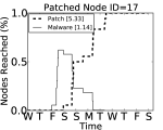
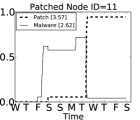
Since the betweenness based containment scheme is not effective, we now evaluate the closeness based spreading scheme with the aim of disseminating a patch message throughout the network more quickly than a malicious message. For brevity, we do not present results on spreading based on temporal betweeness centrality since it is intuitive that this metric is not designed to quantify the speed of the patching dissemination process and, for this reason, it leads to poorer results. We start our analysis by examining a worst case scenario using the CAMBRIDGE dataset: a researcher receives a malicious message on their device in the early hours of Friday morning (=Fri 12am) and the malicious program replicates itself to any devices it meets during the day. A patch message is started a day later to try and patch all the compromised devices (=Sat 12am). This can be considered as the a worst case since there are more interactions and hence more opportunity for malware to spread during the day and the patch is delayed until a day later.
Figure 8 shows the spreading rate for the malicious message versus the best (left) and worst device (right) to start the patching message. These results were obtained by running simulations considering every single device as a starting point of the patching process, and then ranking them based on three performance metrics:
-
•
the area under the curve (AUC), which captures the behaviour of the infection over time with respect to the number of infected devices222The AUC is commonly used in epidemiology and medical trials trials_small_2001 .;
-
•
the peak number of compromised devices ();
-
•
the time in days necessary to achieve total malware containment ().
Since the AUC captures both the and , the best and worst initial devices that were patched were selected using the AUC. Comparing all three measures, the case related to the selection of the worst device (right panel) is characterised by double AUC (2.62 vs. 1.07); a higher peak in compromised devices (68% vs. 60%) and by the fact that it is not possible to fully contain the malware in a finite time ( vs. 3.3 days).
 |
 |
 |
|
4.7 Sensitivity to Malware Start Time
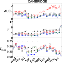
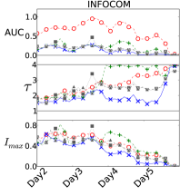
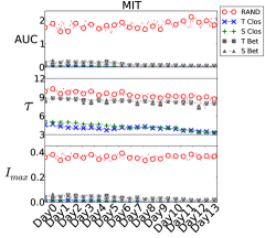
Thus far we have only considered a single malware start time. We now take a broader view and examine the effects of a malicious message starting at different times. For each dataset the AUC, and are exhaustively calculated for different malware start times at hourly intervals and increasing patch delays starting from zero (i.e., patch messages start at the same time as malicious messages) to up to 2 days. As a baseline, a naive method of randomly selecting patching nodes is also calculated, averaged over 100 runs. Figure 9 shows for each dataset the performance metrics as a function of the malware start time , averaged over all patch delays. In particular, we note that the AUC and the maximum number of infected nodes tend to follow the temporal efficiency (strictly related to human circadian rhythms); however, the total time of containment () remains stable across all start times. These results demonstrate that this time-aware containment scheme is an effective method of quickly containing malware, irrespective of when the malware started. Now analysing the AUC and , the temporal centrality curve is consistently lower than static and naive methods. Furthermore, static centrality performs worse than the naive method at some points of time; more specifically:
-
•
For the CAMBRIDGE dataset, during the weekend a static method has a higher peak number of compromised devices () than the naive method, which shows that a static method is not effective at slowing down the malware from spreading.
-
•
For the INFOCOM dataset, again is higher than the naive method, during days 2 and 4. In addition, the AUC curve for a static method peaks with temporal efficiency during days 2, 4 and 5: this means that the malware is not contained effectively in these scenarios. Also, the total containment time () is greater than that of the naive method during days 3, 4 and 5. This shows that temporal centrality is more consistently effective for identifying the best nodes to start the patching process, compared to both static and naive methods.
-
•
Finally, for the MIT dataset, the naive method performs extremely poorly (with high values of UAC, and across all malware start times), compared to either a static or temporal method.
4.8 Summary of the Findings
This study demonstrates that a temporal analysis of mobile device interactions is better suited to real networks where the topology changes over time. As we have seen, a traditional strategy of patching high betweenness nodes is not effective when temporal topological information is taking into account for both the information dissemination process and also centrality calculations. Instead, we propose a strategy that can select the best devices to spread the patch in a competitive fashion, using the same opportunistic encounters with other devices utilised by the malware itself.
5 Epidemics and Immunisation
A promising application area of the proposed metrics is indeed epidemics modelling in human networks May06:network ; KeeRoh07:Modeling . Currently, the vast majority of the existing models assume an underlying static network LEA03:sexual ; Newman10:Networks . By considering a static network, the temporal order of appearance of the links (i.e., the sequence of the contact opportunities) is somehow neglected. This fact might have significant implications on the actual realism of the mathematical model, especially in the case of small populations. Another specific aspect that might have a strong influence on the resulting model is the type of mixing patterns New03:mixing that are present in the population.
The problem of modelling the spreading of infection in a time-varying graph and the definition of vaccination strategies given the information related to the network and epidemic dynamics (and the correlation between the two) are open and challenging research areas at the same time. Temporal centrality metrics can be used for example to prioritise the vaccination of individuals involved in an immunisation program. Moreover, temporal metrics can be used in general to study the evolution of a disease over time by providing quantitative measures of the time scale of its spreading considering the sequence of infected individuals (or geographic areas) over time.
In the recent years, some works have been focussed on the interplay between changing topology and the epidemic process taking place over the network. For example, in SarKas05:modelling Saramäki and Kaski present a model for studying the spreading of an infectious influenza on a dynamic small-world network, by analysing the effect of a dynamic re-wiring process on a Susceptible-Infective-Recovered-style epidemic model, deriving the equations for the the epidemic threshold and spreading dynamics. In particular, the authors show how the epidemic saturation time scale varies with the size of the network and the initial conditions. In LRLH12:exploiting the authors present the results of different vaccination strategies by simulating the dynamics of sexual disease spreading in empirical contact sequences of individuals. More specifically, the authors analyse the largest outbreak, the average outbreak sizes, and the relative advantages of the different strategies as a function of the infectivity and the duration of the infective state.
In general, social encounter networks, a typical class of time-varying networks, are attracting an increasing attention in the epidemiology community DHRK12:social . Researchers have been employing RFID and sensor techniques for extracting contact traces in order to accurately reconstruct patterns of interactions among individuals, also with respect to the duration of the contacts (see for example CHCDGS07:impact ; CVBCP10:Dynamics ; SKLLFJ10:highresolution ). These models might also be scaled up to study disease outbreaks in cities EGAMSTW04:modelling .
Epidemic models have also been applied to diffusion of ideas, behaviour or lifestyle choices in social networks Cen10:spread , for example in order to study the spreading of obesity ChrFow07:spread or smoking ChrFow08:collective . Another interesting and open area is the characterisation of the spreading of an epidemic and the simultaneous dissemination of information about it that might modify the behaviour of individuals (i.e., the dynamics of the underlying time-varying networks). A work in this direction is FGWJ09:spread .
We believe that the application of the proposed metrics to these fields is indeed very promising and might contribute to increase the accuracy, and therefore, the realism of existing models and to develop new ones allowing researchers to extract valuable information and insights from them. In particular, the centrality metrics presented in this chapter and the accompanying one NTMMRL12:graphs in this book can be used to identify the key spreaders in order to define effective containment and immunisation strategies. For example, vaccination can be based on priorities assigned to the temporal centralities of the individuals in case of human diseases, whereas, as far as computer viruses are concerned, white worms used for patching the systems could be distributed starting from the nodes with the highest temporal closeness centrality.
6 Final Remarks
In this chapter we presented some key applications of temporal metrics to various domains such as centrality analysis in a social network, robustness and epidemiology of computer viruses and diseases. We have shown that temporal graph metrics are able to provide information about the structure of the time-varying networks and the dynamics of processes happening over them that is not possible to extract through the classic static metrics and graph representations. We hope that the case studies presented in this chapter and the discussions of open problems in the field might be considered as a starting point and a source of inspiration for future applications in these and other fields.
Acknowledgements.
This work was funded in part through EPSRC Project MOLTEN (EP/I017321/1) and the EU LASAGNE Project, Contract No.318132 (STREP).References
-
[1]
Virus description: Bluetooth-worm:symos/cabir.
http://www.f-secure.com/v-descs/cabir.shtml, 2004. - [2] Reka Albert, Hawoong Jeong, and Albert-Laszlo Barabási. Error and attack tolerance of complex networks. Nature, 406(6794):378–382, July 2000.
- [3] Alain Barrat, Marc Barthélemy, and Alessandro Vespignani. Dynamical Processes on Complex Networks. Cambridge University Press, November 2008.
- [4] Stefano Boccaletti, Vito Latora, Yamir Moreno, Mario Chavez, and Dong-Uk Hwang. Complex networks: Structure and dynamics. Physics Reports, 424(4-5):175–308, February 2006.
- [5] Duncan S. Callaway, M. E. J. Newman, Steven H. Strogatz, and Duncan J. Watts. Network robustness and fragility: Percolation on random graphs. Physical Review Letters, 85(25):5468–5471, Dec 2000.
- [6] Ciro Cattuto, Wouter Van den Broeck, Alain Barrat, Vittoria Colizza, Jean-Francois Pinton, and Alessandro Vespignani. Dynamics of Person-to-Person Interactions from Distributed RFID Sensor Networks. PLoS ONE, 5(7):e11596, 07 2010.
- [7] CBS News. Enron traders caught on tape. http://www.cbsnews.com/stories/2004/06/01/ eveningnews/main620626.shtml, June 2004.
- [8] CBS News. Former Enron Trader Pleads Guilty. http://www.cbsnews.com/stories/2004/06/16/ national/main623569.shtml, August 2004.
- [9] Damon Centola. The spread of behavior in an online social network experiment. Science, 329(5996):1194–1197, 2010.
- [10] Augustin Chaintreau, Pan Hui, Jon Crowcroft, Christophe Diot, Richard Gass, and James Scott. Impact of Human Mobility on Opportunistic Forwarding Algorithms. IEEE Trans. on Mobile Computing, 6(6):606–620, 2007.
- [11] Augustin Chaintreau, Pan Hui, Jon Crowcroft, Christophe Diot, Richard Gass, and James Scott. Impact of Human Mobility on Opportunistic Forwarding Algorithms. IEEE Transactions on Mobile Computing, 6(6):606–620, june 2007.
- [12] Augustin Chaintreau, Jean Y. Le Boudec, and Nikodin Ristanovic. The age of gossip: spatial mean field regime. In Proceedings of SIGMETRICS ’09, pages 109–120, New York, NY, USA, 2009. ACM.
- [13] Nicholas A. Christakis and James H. Fowler. The Spread of Obesity in a Large Social Network over 32 Years. New England Journal of Medicine, 357(4):370–379, 2007.
- [14] Nicholas A. Christakis and James H. Fowler. The Collective Dynamics of Smoking in a Large Social Network. New England Journal of Medicine, 358(21):2249–2258, 2008.
- [15] Aaron Clauset and Nathang Eagle. Persistence and Periodicity in a Dynamic Proximity Network. In Proceedings of DIMACS Workshop on Computational Methods for Dynamic Interaction Networks, September 2007.
- [16] Paolo Crucitti, Vito Latora, Massimo Marchiori, and Andrea Rapisarda. Error and attack tolerance of complex networks. Physica A, 340:388–394, 2004.
- [17] Leon Danon, Thomas A. House, Jonathan M. Read, and Matt J. Keeling. Social encounter networks: collective properties and disease transmission. Journal of the Royal Society Interface, 9(76), 11 2012.
- [18] N. Eagle and A. Pentland. Reality Mining: Sensing Complex Social Systems. Personal Ubiquitous Comput., 10(4):255–268, 2006.
- [19] Peter Elkind and Bethany McLean. The Smartest Guys in the Room: The Amazing Rise and Scandalous Fall of Enron. Penguin, September 2004.
- [20] Paul Erdős and Alfred Rényi. On the evolution of random graphs. Publications of the Mathematical Institute of the Hungarian Academy of Sciences, 5:17–61, 1960.
- [21] Stephen Eubank, Hasan Guclu, V. S. Anil Kumar, Madhav V. Marathe, Aravind Srinivasan, Zoltan Toroczkai, and Nan Wang. Modelling disease outbreaks in realistic urban social networks. Nature, 429(6988):180–184, 05 2004.
- [22] Charles H. Evans, Jr. and Suzanne T. Ildstad. Small Clinical Trials: Issues and Challenges. National Academy of Sciences Press, January 2001.
- [23] Michalis Faloutsos, Petros Faloutsos, and Christos Faloutsos. On power-law relationships of the Internet topology. In Proceedings of SIGCOMM ’99, pages 251–262, New York, NY, USA, 1999. ACM.
- [24] Federal Energy Regulatory Commission. Addressing the 2000-2001 Western Energy Crisis, December 2008.
- [25] Sebastian Funka, Erez Gilada, Chris Watkinsb, and Vincent A. A. Jansena. The spread of awareness and its impact on epidemic outbreaks. PNAS, 106:6872–7, April 2009.
- [26] Christos Gkantsidis, Thomas Karagiannis, and Milan Vojnovic. Planet scale software updates. In Proceedings of SIGCOMM ’06, New York, NY, USA, 2006. ACM.
- [27] P. Holme, B. J. Kim, C. N. Yoon, and S. K. Han. Attack vulnerability of complex networks. Phys. Rev. E, 65(5), May 2002.
- [28] Bernardo A. Huberman and Lada A. Adamic. Growth dynamics of the world-wide web. Nature, 401(6749):131, 1999.
- [29] Mikko Hypponen. F-secure weblog: The grand opening!, May 2005.
- [30] Matt J. Keeling and Pei Rohani. Modeling Infectious Diseases in Human and Animals. Princeton University Press, 2007.
- [31] David Kempe, Jon Kleinberg, and Amit Kumar. Connectivity and inference problems for temporal networks. In J. Comput. Syst. Sci, page 2002, 2000.
- [32] Maurice G. Kendall. A new measure of rank correlation. Biometrika, 30(1-2):81–93, 1938.
- [33] V. Kostakos. Temporal graphs. Physica A, 388(6):1007–1023, March 2009.
- [34] Neal Leavitt. Mobile phones: the next frontier for hackers? Computer, 38(4):20–23, 2005.
- [35] Sungmin Lee, Luis E. C. Rocha, Fredrik Liljeros, and Petter Holme. Exploiting temporal network structures of human interaction to effectively immunize populations. PLoS ONE, 7:e36439, 05 2012.
- [36] Fredrik Liljeros, Christofer R. Edling, and Luis A.Nunes Amaral. Sexual networks: implications for the transmission of sexually transmitted infections. Microbes and Infection, 5(2):189 – 196, 2003.
- [37] Robert M. May. Network structure and the biology of populations. Trends in Ecology and Evolution, 1, July 2006.
- [38] Alberto Medina, Gonca Gursun, Prithwish Basu, and Ibrahim Matta. On the Universal Generation of Mobility Models. In Proceedings of IEEE/ACM MASCOTS ’10, Miami Beach, FL, US, August 2010.
- [39] Mark Newman. Networks: An Introduction. Oxford University Press, 2010.
- [40] Mark E. J. Newman. Mixing patterns in networks. Phys. Rev. E, 67:026126, Feb 2003.
- [41] Vincenzo Nicosia, John Tang, Cecilia Mascolo, Mirco Musolesi, Giovanni Russo, and Vito Latora. Graph metrics for temporal networks. In Jari Saramäki and Petter Holme, editors, Temporal Networks. Springer, 2013.
- [42] Michal Piorkowski, Natasa Sarafijanovic-Djukic, and Matthias Grossglauser. CRAWDAD data set epfl/mobility (v. 2009-02-24). Downloaded from http://crawdad.cs.dartmouth.edu/epfl/mobility, February 2009.
- [43] Cabspotting Project. http://cabspotting.org/.
- [44] K. K. Rachuri, M. Musolesi, C. Mascolo, P. J. Rentfrow, C. Longworth, and A. Aucinas. EmotionSense: a mobile phones based adaptive platform for experimental social psychology research. In Proceedings of UbiComp ’10, September 2010.
- [45] E. Van Ruitenbeek, T. Courtney, W.H. Sanders, and F. Stevens. Quantifying the effectiveness of mobile phone virus response mechanisms. In Proceedings of DNS ’07, 2007.
- [46] Marcel Salathé, Maria Kazandjieva, Jung W. Lee, Philip Levis, Marcus W. Feldman, and James H. Jones. A high-resolution human contact network for infectious disease transmission. Proceedings of the National Academy of Sciences, 107:22020–22025, December 2010.
- [47] Jari Saramäki and Kimmo Kaski. Modelling development of epidemics with dynamic small-world networks. Journal of Theoretical Biology, 234(3):413 – 421, 2005.
- [48] Salvatore Scellato, Ilias Leontiadis, Cecilia Mascolo, Pritwish Basu, and Murtaza Zafer. Evaluating Temporal Robustness of Mobile Networks. IEEE Transactions on Mobile Computing. http://doi.ieeecomputersociety.org/10.1109/TMC.2011.248.
- [49] James Scott, Richard Gass, Jon Crowcroft, Pan Hui, Christophe Diot, and Augustin Chaintreau. CRAWDAD data set cambridge/haggle (v. 2009-05-29). Downloaded from http://crawdad.cs.dartmouth.edu/cambridge/haggle, May 2009.
- [50] Jitesh Shetty and Jafar Adibi. Discovering important nodes through graph entropy the case of Enron email database. In Proceedings of the 3rd International Workshop on Link Discovery, pages 74–81, Chicago, Illinois, 2005. ACM.
- [51] John Tang, Hyoungshick Kim, Cecilia Mascolo, and Mirco Musolesi. STOP: Socio-Temporal Opportunistic Patching of Short Range Mobile Malware. In Proceedings of the 13th IEEE Symposium on a World of Wireless, Mobile and Multimedia Networks (WOWMOM’12), San Francisco, California, USA, June 2012.
- [52] John Tang, Cecilia Mascolo, Mirco Musolesi, and Vito Latora. Exploiting Temporal Complex Network Metrics in Mobile Malware Containment. In Proceedings of the 12th IEEE International Symposium on a World of Wireless, Mobile and Multimedia Networks (WOWMOM’11), Lucca, Italy, June 2011.
- [53] John Tang, Mirco Musolesi, Cecilia Mascolo, and Vito Latora. Temporal Distance Metrics for Social Network Analysis. In Proceedings of WOSN ’09, Barcelona, Spain, August 2009.
- [54] John Tang, Mirco Musolesi, Cecilia Mascolo, Vito Latora, and Vincenzo Nicosia. Analysing information flows and key mediators through temporal centrality metrics. In Proceedings of ACM SNS ’10, Paris, France, April 2010.
- [55] Pu Wang, Marta C. Gonzalez, Cesar A. Hidalgo, and Albert-Laszlo Barabasi. Understanding the spreading patterns of mobile phone viruses. Science, 324(5930):1071–1076, May 2009.
- [56] Washington Post. Enron fraud trial ends in 5 convictions. http://www.washingtonpost.com/wp-dyn/articles/A23034-2004Nov3.html.
- [57] Stanley Wasserman and Katherine Faust. Social Networks Analysis. Cambridge University Press, 1994.
- [58] Zhichao Zhu, Guohong Cao, Sencun Zhu, Supranamaya Ranjan, and Antonio Nucci. A social network based patching scheme for worm containment in cellular networks. In Proceedings of INFOCOM ’09, Rio de Janeiro, Brazil, April 2009. IEEE.
- [59] Gjergji Zyba, Geoffrey M. Voelker, Michael Liljenstam, Andras Mehes, and Per Johansson. Defending mobile phones from proximity malware. In Proceedings of INFOCOM ’09, Rio de Janeiro, Brazil, April 2009. IEEE.