Recurrence Statistics of Great Earthquakes

Abstract

We investigate the sequence of great earthquakes over the past century. To examine whether the earthquake record includes temporal clustering, we identify aftershocks and remove those from the record. We focus on the recurrence time, defined as the time between two consecutive earthquakes. We study the variance in the recurrence time and the maximal recurrence time. Using these quantities, we compare the earthquake record with sequences of random events, generated by numerical simulations, while systematically varying the minimal earthquake magnitude $M_{\rm min}$. Our analysis shows that the earthquake record is consistent with a random process for magnitude thresholds $7.0\leq M_{\rm min}\leq 8.3$, where the number of events is larger. Interestingly, the earthquake record deviates from a random process at magnitude threshold $8.4\leq M_{\rm min}\leq 8.5$, where the number of events is smaller; however, this deviation is not strong enough to conclude that great earthquakes are clustered. Overall, the findings are robust both qualitatively and quantitatively as statistics of extreme values and moment analysis yield remarkably similar results.

I Introduction

Remote triggering of large earthquakes, where one large earthquake causes another large earthquake at a global distance comparable to the size of the earth, is the subject of ongoing debate in geophysics. It is well known that earthquakes do cause aftershocks on local scales, at distances comparable to the size of the fault. In the last 20 years, it has been shown that seismic waves can dynamically trigger earthquakes at large distances (Hill et al. , 1993; Gomberg et al. , 2004; Freed, 2005), and more recently, that a large earthquake can trigger other large earthquakes at global distances (Pollitz et al. , 2012). However, other recent studies suggest that dynamic triggering of large earthquakes is not widespread (Parsons and Velasco, 2011; van der Elst et al. , 2013). Thus, dynamic triggering of large events at global distances remains an open question, one with potentially significant implications for hazard analysis and earthquake physics.

Remote triggering necessarily implies that large earthquakes are correlated in time, that is, earthquakes are not equivalent to a random process. The increase in earthquake activity over the past decade including three of the six largest events on record over the past century (Brodsky, 2009; Ammon et al. , 2011) raises the question whether great earthquake are clustered (Fig. 1).

Recent studies have utilized a variety of statistical methods to examine whether the sequence of large earthquakes is consistent with a random process. The approaches used to analyze the earthquake record include for example, statistics of the number of events in a fixed time interval, and statistics of the time between events. However, the small number of powerful events constitutes a serious challenge for such investigations (Kerr, 2011; Dimer de Oliveira, 2012). To date, some studies reported deviations from random event statistics (Bufe and Perkins, 2005, 2011), while several others report that the earthquake record is consistent with random statistics (Michael, 2011; Shearer and Stark, 2012; Parsons and Geist, 2012; Daub et al. , 2012).

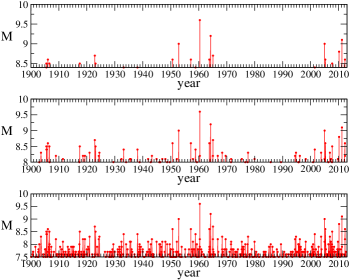
Figure 1: The sequence of large earthquakes during the years $1900-2012$. Three thresholds are used: $M_{\rm min}=7.5$ (bottom), $M_{\rm min}=8.0$ (middle), and $M_{\rm min}=8.5$ (top).

In this study, we focus on the recurrence time between successive earthquake events, a quantity that allows us to probe the most powerful events on record. Our statistical analysis quantifies typical properties as well as extremal properties of the recurrence time. Using numerical simulations, we generate a large number of random sequences, thereby allowing probabilistic comparison between the earthquake record and a random process.

II Earthquake record

We analyze the earthquake event times in the USGS PAGER (Prompt Assessment of Global Earthquake Response) catalog (Allen et al. , 2009), supplemented by the Global CMT (Centroid Moment Tensor) catalog (Ekström et al., 2012). These two catalogs comprise a global record from 1900 through December 31, 2012, containing 1770 events with magnitude $M\geq 7$ (Table I).

$M_{\rm min}$	All events	Aftershocks removed
7.0	1770	1255
7.5	447	371
8.0	84	74
8.5	19	17
9.0	5	5
9.5	1	1

Table 1: The number of large events on record during the years $1900-2012$. Listed are the total number of events (with and without aftershocks) versus the minimum magnitude $M_{\rm min}$.

The catalog contains aftershocks, which must be identified to address whether earthquake occurrence is random over global distances. Removal of aftershocks is not a trivial procedure, as it requires assumptions that cannot be tested due to limited data (Marsan and Lengliné, 2008). We identify aftershocks using a window method (Gardner and Knopoff, 1974): any event close enough to another larger event in both space and time is considered an aftershock, and is removed from the catalog. We examine a variety of choices for the distance and time windows and verify that our conclusions are robust with respect to the aftershock removal procedure. In the following, we use the time window in the original Gardner and Knopoff study, and our choice for the distance window is a purposely conservative estimate of the rupture length for a given magnitude (i.e. overestimated spatial extent of aftershocks), based on an empirical law (Wells and Coppersmith, 1994). We note that our analysis classifies two of the $M=8.5$ events as aftershocks: the $M=8.6$ 2005 Nias earthquake, and the $M=8.5$ 2007 Sumatra earthquake, both aftershocks of the 2004 $M=9.0$ Sumatra-Andaman earthquake. Without aftershocks, the catalog contains 1255 events (Table 1). For completeness, we include in our investigation both the raw earthquake catalog as well as the catalog with aftershocks removed.

III Recurrence Statistics

The basic quantity in our analysis is the recurrence time, defined as the time between two successive events. Recurrence times are commonly used to characterize seismic activity. For a random process, where events occur at a constant rate and there are no correlations between different events, the cumulative distribution $P(t)$ of recurrence intervals that are larger than $t$ is purely exponential,

$$P(t)=\exp\left(-t/\langle t\rangle\right).$$ (1)

Here, $\langle t\rangle$ is the average recurrence time.

For reference, the distribution (1) with the average $\langle t\rangle$ calculated from the empirical data is also shown in figure 2. The empirical distribution is in good agreement with the exponential distribution for magnitude thresholds $M_{\rm min}=7.0$, $M_{\rm min}=7.5$, and $M_{\rm min}=8.0$. In two cases ($M_{\rm min}=7.0$ and $M_{\rm min}=8.0$) the tail of the distribution becomes closer to an exponential once aftershocks are removed. This preliminary analysis indicates that the sequence of large earthquake events does not show significant deviations from random event statistics.

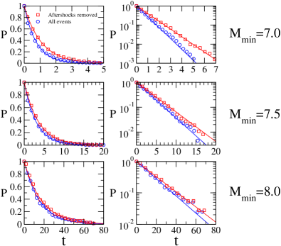
Figure 2: The cumulative distribution of recurrence time versus time (in months). Data for all events is shown in circles and data for the earthquake catalog without aftershocks is shown in squares. The line displays an exponential distribution, where the average recurrence time matches the empirical value.

As the magnitude threshold increases, the number of events becomes smaller and the distribution of recurrence times can be probed only over a smaller range. Consequently, the tail of the distribution, which quantifies the likelihood of large gaps between events, becomes difficult to measure. To address this issue and to systematically probe high magnitudes, we analyze a standard measure for fluctuations, the normalized variance

$$V=\frac{\langle t^{2}\rangle-\langle t\rangle^{2}}{\langle t\rangle^{2}}.$$ (2)

Here the bracket denotes an average over all recurrence intervals in the sequence. The variance involves the lowest (nontrivial) integer moment of the distribution, yet, as discussed below, we also analyze a range of other moments.

We use numerical simulations to characterize how the normalized variance behaves for a random process. We generate a very large number ($10^{8}$) of random sequences where the recurrence times are identical and independently distributed variables, drawn from the exponential distribution (1). The number of events $N$ and the average recurrence time $\langle t\rangle$ are set by the earthquake record, for each magnitude threshold $M_{\rm min}$. By simulating the precise number of events $N$ on record, our analysis properly quantifies the large fluctuations that are expected when the number of events is small.

We measure the average variance, $\langle V\rangle$, and the standard deviation in the variance, $\delta V$, defined by $(\delta V)^{2}=\langle V^{2}\rangle-\langle V\rangle^{2}$ (here, the bracket denotes an average over all random sequences). As shown in figure 3a, the normalized variance is close to unity when the number of events is large, but when the number of events is small (at large magnitudes), the expected variance decreases, and the standard deviation becomes comparable to the mean. We also confirm that as expected, $\delta V\sim N^{-1/2}$ for large $N$.

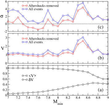
Figure 3: (a) The average variance $\langle V\rangle$ and the standard deviation of the variance $\delta V$ as a function of magnitude threshold $M_{\rm min}$. These quantities correspond to a random sequence with a number of events that matches that of the earthquake record (aftershocks removed). (b) Normalized variance $V$ as a function of $M_{\rm min}$. Shown are the behaviors with and without aftershocks. (c) The number of standard deviations away from the mean $\sigma$ defined in Eq. (3), versus $M_{\rm min}$.

The normalized variance defined in Eq. (2) is shown as a function of the threshold magnitude in Fig. 3b. Using the average $\langle V\rangle$ and the standard deviation $\delta V$ obtained from simulated sequences, we also calculate $\sigma$ the number of standard deviations away from the mean (Fig. 3c),

$$\sigma=\frac{V-\langle V\rangle}{\delta V}.$$ (3)

For most magnitude thresholds, even without removing aftershocks, the quantity $\sigma$ is not large, evidence that the earthquake sequence is consistent with a random process. There are however three significant peaks that indicate potential deviations from random event statistics. First, at the magnitude thresholds $7.0\leq M_{\rm min}\leq 7.2$, the raw earthquake catalog deviates from a random process, but once aftershocks are removed, these deviations are largely eliminated. Second, there is a peak at $M_{\rm min}=7.8$, but again, this peak is eliminated once aftershocks are removed. Third, the most pronounced peak occurs when $8.4\leq M_{\rm min}\leq 8.5$. In this case, however, removing aftershocks diminishes the magnitude of the peak only slightly (for such powerful earthquakes, aftershocks are of course rare, see Table 1).

Figure 4: The fraction $F_{V}$ of random sequences with variance exceeding the empirical value versus magnitude threshold $M_{\rm min}$. Shown are results for the raw catalog (circles) and the catalog with aftershocks removed (squares). The error bars were produced using the moment analysis described in the main text.

To quantify the significance of the peaks in the quantity $\sigma$, we use probabilistic analysis. Such analysis requires numerical simulations because the distribution of the variance depends strongly on the number of events: this distribution approaches a normal distribution as the number of events becomes very large, but it is much broader when the number of events is small. Specifically, we measure the fraction $F_{V}$ of simulated random sequences where the normalized variance exceeds the empirical value $V$. Figure 4 shows the fraction $F_{V}$ as a function of magnitude threshold $M_{\rm min}$. For each peak in $\sigma$, there is a corresponding dip in the fraction $F_{V}$. These dips are mostly suppressed once aftershocks are removed. Yet, the dip at the narrow band $8.4\leq M_{\rm min}\leq 8.5$ is robust. At $M_{\rm min}=8.5$ we find $F_{V}\approx 1/300$, that is, only one in about $300$ random sequences has a variance that exceeds that of the earthquake data. This small fraction implies that the earthquake record deviates from a random process at this particular magnitude threshold. As pointed out by Shearer and Stark Shearer and Stark (2012), because $M_{\rm min}=8.5$ is chosen a posteriori, the measured fraction $F_{V}$ may represent an underestimate. Regardless, the fraction $F_{V}$ is not sufficiently small to conclude with confidence that the earthquake record violates random statistics or equivalently, that there are temporal correlations (or causal relationships) between large events.

As a reference, our simulations show if $3$, $6$, or $9$ additional $M\geq 8.5$ events occur over the next decade (Shearer and Stark, 2012), the quantity $F_{V}$ would then drop to $1.8\times 10^{-3}$, $2.9\times 10^{-4}$, and $9\times 10^{-5}$, respectively. The change in the quantity $F_{V}$ with even a few additional events illustrates the uncertainties associated with such small catalogs.

For further insight, we examine statistical properties of the maximal recurrence time $t_{\rm max}$, corresponding to the longest quiescent period between consecutive earthquakes. Similar to the probabilistic analysis above, we measure the fraction $F_{\rm max}$ of random sequences where the maximal recurrence time exceeds $t_{\rm max}$. When the number of events is large, this fraction is given by the formula $F_{\rm max}=1-[1-\exp(-t/\langle t\rangle)]^{N}$. Fig. 5a shows the fraction $F_{\rm max}$ as a function of $M_{\rm min}$. Statistics of the largest recurrence time are strongly correlated with those of the variance: the fraction $F_{\rm max}$ mirrors the behavior of the fraction $F_{V}$ (Figures 4 and 5a). Moreover, if we restrict our attention to magnitudes $M_{\rm min}\geq 7.7$ where aftershocks are rare, the two fractions are remarkably close to each other (figure 5b). Indeed, we verify that simulated random sequences with a maximal gap that exceeds $t_{\rm max}$ also have variance that exceeds $V$. This extreme event analysis demonstrates that the very large $39.9$ year gap separating two clusters of activity, one during 1950-1965 and one during 2004-2012 is responsible for the anomalously large variability observed at the magnitude threshold $M_{\rm min}=8.5$ (figure 1).

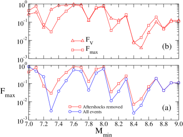
Figure 5: (a) Fraction $F_{\rm max}$ of random sequences where the maximal recurrence time exceeds the largest recurrence time on record versus magnitude threshold $M_{\rm min}$. (b) The fraction $F_{V}$ (see also figure 4) and the fraction $F_{\rm max}$ for the earthquake catalog without aftershocks.

Previous statistical analysis based on the number of events in a given time interval revealed deviations from random event statistics at this magnitude range that can be traced to magnitude uncertainties in the earlier part of the century (Daub et al. , 2012). To assess the effects of uncertainties in the earthquake magnitude (Engdahl and Villasenor, 2002), we introduce unbiased variations in the magnitude: $M\to M+\delta M$ where $\delta M$ represents a potential measurement error. The quantity $\delta M$ is drawn from a uniform distribution in the range $[-\Delta M:\Delta M]$. We systematically increase the range $\Delta M$ up to as high as $\Delta M=0.8$, and repeat the analysis used to obtain figures 3-5. Each data point is obtained using $10^{8}$ simulated catalogs: $10^{4}$ distinct modifications of the original earthquakes catalog were generated, and for each modification, $10^{4}$ simulated catalogs were produced. The fractions $F_{V}$ and $F_{\rm max}$ become smoother as the range $\Delta M$ increases (Figure 6), and moreover, the dips at $M=8.5$ are strongly suppressed. We also consider situations where the magnitude is always underestimated or overestimated by uniformly drawing $\delta M$ in the range $[0:\Delta M]$ or $[-\Delta M:0]$. Biased errors lead to the same patterns shown in figure 6. We also verify that variations $\delta M$ drawn from a normal distribution with standard deviation $\Delta M$ lead to similar results. Consistent with Ref. (Parsons and Geist, 2012), magnitude uncertainty analysis supports the conclusions of our statistical analysis.

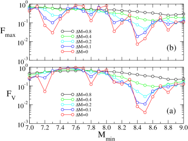
Figure 6: Magnitude uncertainty analysis for the earthquake catalog (aftershocks removed). Shown are: (a) The quantity $F_{V}$ as in figure 4 and (b) the quantity $F_{\rm max}$ as in figure 5 versus $M_{\rm min}$. The quantity $\Delta M$ quantifies the range of magnitude uncertainty, and the different curves represent different values of $\Delta M$ in the plots.

To examine whether the results are sensitive to the particular measure of variability (2), we repeat the analysis using the normalized moments $M_{n}=\langle t^{n}\rangle/\langle t\rangle^{n}$ instead of the variance $V=M_{2}-1$. We examine a series of moments in the range $1.25\leq n\leq 4$ and again, measure the fraction $F_{M}$ of simulated catalogs where the moment $M_{n}$ exceeds the value measured for the earthquake data. By varying the parameter $n$ and identifying the maximal and minimal fractions $F_{M}$, we produce the error bars shown in figure 4. The results of this moment analysis confirm that the dips in the quantity $F_{V}$ are robust.

IV Conclusions

In summary, we analyzed typical and extremal properties of the time intervals between large earthquakes. The results of our statistical tests reconcile recent studies that address the question: “are great earthquakes clustered?” Our study yields three important conclusions.

First, in the magnitude threshold range $7.0\leq M_{\rm min}\leq 8.3$ which constitutes the vast majority of great earthquakes on record, the earthquake sequence does not exhibit significant deviations from a random set of events. These findings reinforce the results of several studies (Michael, 2011; Shearer and Stark, 2012; Parsons and Velasco, 2011; Daub et al. , 2012). At several threshold magnitudes, the earthquake record is consistent with a random process even if aftershocks are not removed from the catalog.

Second, the roughly twenty most powerful events on record, corresponding to magnitude threshold $8.4\leq M_{\rm min}\leq 8.5$, deviate from a random sequence of events. This departure is tied to the anomalously long gap between two clusters of events, one in the mid-century, and one over the past decade, an observation also noted in (Bufe and Perkins, 2005, 2011; Shearer and Stark, 2012). However, this departure is not sufficiently strong to conclude that there are temporal correlations between great earthquakes: the likelihood that a random sequence matches the variability in the data ($\approx 1/300$) is equivalent to only $\approx 2.6$ standard deviations from the mean for a normal distribution.

Third, the results are qualitatively and quantitatively robust. Analysis of average properties and analysis of extremal properties of the recurrence time leads not only to similar conclusions, but also, to very similar likelihood figures that the observed sequence of events can be explained by a random process. We have also considered magnitude uncertainties using unbiased and biased measurement errors in earthquake magnitude and observed that such errors systematically suppress deviations from random event statistics.

Finally, our study uses the average recurrence time as a measure for the overall rate of events. Uncertainties in the overall rate of events are significant when the number of events is small, and an important challenge for future research is to generalize the analysis above to incorporate uncertainties in the overall rate of events.

We thank Robert Guyer, Robert Ecke, Joan Gomberg, and Thorne Lay for comments. We gratefully acknowledge support for this research through DOE grant DE-AC52-06NA25396.

References

- Hill et al. (1993) Hill, D. P., et al. (1993), Remote seismicity triggered by the M7.5 Landers, California earthquake of June 28, 1992, Science 260, 1617-1623.
- Gomberg et al. (2004) Gomberg, J., P. Bodin, K. Larson, and H. Dragert (2004), Earthquake nucleation by transient deformations caused by the Denali, Alaska, earthquake, Nature 427, 621-624.
- Freed (2005) Freed, A. M. (2005), Earthquake triggering by static dynamic, and postseismic stress transfer, Ann. Rev. Earth Plant. Sci. 33, 335-367.
- Pollitz et al. (2012) Pollitz F. F. ,R. S. Stein, V. Sevilgen, and R. Burgmann (2012), The 11 April 2012 east Indian Ocean earthquake triggered large aftershocks worldwide, Nature 490, 250.
- van der Elst et al. (2013) van der Elst, N. J., E. M. Brodsky, and T. Lay, (2013), Remote Triggering Not Evident Near Epicenters of Impending Great Earthquakes, Bull. Seismol. Soc. Am. 103, 1522-1540.
- Parsons and Velasco (2011) Parsons, T., and A. A. velasco (2011), Absence of remotely triggered large earthquakes beyond the mainshock region, Nat. Geosci. 4, 312-316.
- Ammon et al. (2011) Ammon, C. J., R. C. Aster, T. Lay, and D. W. Simpson (2011), The Tohoku Earthquake and a 110-year Spatiotemporal Record of Global Seismic Strain Release, Seismol. Res. Lett. 82, 455.
- Brodsky (2009) Brodsky, E. E. (2009), The 2004-2008 Worldwide Superswarm, Eos. Trans. AGU, Fall Meet. Suppl., 90, S53B.
- Dimer de Oliveira (2012) Dimer de Oliveira, F. (2012), Can we trust earthquake cluster detection tests?, Geophys. Res. Lett. 39, L052130.
- Kerr (2011) Kerr, R. A. (2011), More Megaquakes on the Way? That Depends on Your Statistics, Science, 332, 411.
- Bufe and Perkins (2005) Bufe, C. G., and D. M. Perkins (2005), Evidence for a Global Seismic-Moment Release Sequence, Bull. Seismol. Soc. Am. 95, 833-843.
- Bufe and Perkins (2011) Bufe, C. G., and D. M. Perkins (2011), The 2011 Tohoku Earthquake: Resumption of Temporal Clustering of Earth’s Megaquakes, Seismol. Res. Lett. 82, 455.
- Parsons and Geist (2012) Parsons, T., and E. L. Geist (2012), Were Global Earthquake Time Intervals Random Between 1900 and 2011?, Bull. Seismol. Soc. Am. 102, 1583-1592.
- Daub et al. (2012) Daub, E. G. , E. Ben-Naim, R. A. Guyer, and P. A. Johnson (2012), Are megaquakes clustered? Geophys. Res. Lett. 39, L06308.
- Michael (2011) Michael, A. J. (2011), Random Variability Explains Apparent Global Clustering of Large Earthquakes, Geophys. Res. Lett. 38, L21301.
- Shearer and Stark (2012) Shearer, P. M., and P. B. Stark, (2012), The global risk of big earthquakes has not recently increased, Proc. Nat. Acad. Sci. 109(3), 717-721.
- Allen et al. (2009) Allen, T. I., K. Marano, P. S. Earle, and D. J. Wald (2009), PAGER-CAT: A composite earthquake catalogue for calibrating global fatality models, Seism. Res. Lett. 80, 50-56.
- Ekström et al. (2012) Ekström, G., M. Nettles, A. M. Dziewonski (2012), The global CMT project 2004-2010: Centroid-moment tensors for 13,017 earthquakes, Phys. Earth Planet. Int. 200-201, 1-9.
- Marsan and Lengliné (2008) Marsan, D., and O. Lengliné (2008), Extending Earthquakes’ Reach Through Cascading, Science 319, 1076-1079.
- Gardner and Knopoff (1974) Gardner, J. K., and L. Knopoff, (1974), Is the sequence of earthquakes in Southern California, with aftershocks removed, Poissonian? Bull. Seismol. Soc. Am. 64, 1363-1367.
- Wells and Coppersmith (1994) Wells, D. L., and K. J. Coppersmith (1994), New empirical relationships among magnitude, rupture length, rupture width, rupture area, and surface displacement, Bull. Seismol. Soc. Am. 84, 1053-1069.
- Engdahl and Villasenor (2002) Engdahl, E. R., and A. Villasenor (2002), Global seismicity: 1900-1999, International Handbook of Earthquake and Engineering Seismology, Volume 81A, ISBN:0-12-440652-1, 665-690.