Thermal drag in spin ladders coupled to phonons

Abstract

We study the spin-phonon drag effect in the magnetothermal transport of spin-1/2 two-leg ladders coupled to lattice degrees of freedom. Using a bond operator description for the triplon excitations of the spin ladder and magnetoelastic coupling to acoustic phonons, we employ the time convolutionless projection operator method to derive expressions for the diagonal and off-diagonal thermal conductivities of the coupled two-component triplon-phonon system. We find that for magnetoelastic coupling strengths and diagonal scattering rates relevant to copper-oxide spin-ladders the drag heat conductivity can be of similar magnitude as the diagonal triplon heat conductivity. Moreover, we show that the drag and diagonal conductivities display very similar overall temperature dependences. Finally, the drag conductivity is shown to be rather susceptible to external magnetic fields.

I Introduction

Understanding spin transport is not only a fundamental issue of quantum many body physics, but also paramount to future spintronics and quantum information processing. A new route into pure spin transport, without mobile charge degrees of freedom has been established a decade by now, with the colossal magnetic heat transport in quasi one-dimensional (1D) spin ladder materials such as (La,Ca,Sr)₁₄Cu₂₄O₄₁ Sologubenko2000a ; Hess2001a ; Kudo2001a - where the magnetic contribution to the total thermal conductivity $\kappa$ exceeds the phonon part substantially - as well as in other 1D spin chain compounds Sologubenko2000a ; Sologubenko2001a ; Hess2007b . This phenomenon has led to an upsurge of interest in the non-equilibrium properties of low-dimensional quantum magnets. Experimentally available data for the spin transport in ladders is analyzed in terms of Boltzmann descriptions suggesting very large low-temperature mean-free paths of several hundred lattice constants Sologubenko2000a ; Hess2001a . This remains ill-understood FHM2007a .

In this context extrinsic scattering, by impurities and phonons may play an important role. Phonons by themselves are omnipresent carriers of heat, which directly interact with spin degrees of freedom, primarily via magnetoelastic coupling. Usually this interaction is treated as a source of dissipation of the spin and phonon heat currents Shimshoni2003a ; Rozhkov2005a ; Chernyshev2005a ; Louis2006a . However, another less well studied consequence of a coupled spin-phonon two-component system exists: namely the off-diagonal effect of the flow of one of the excitations facilitating the flow of the other Gurevich1967a ; Boulat2007a ; Chernyshev2007a . This is referred to as “spin-phonon drag,” in analogy with electron-phonon drag discussed for thermoelectric phenomena in metals and semiconductors Holstein1964a ; Bass1990a ; Gurevich1946a ; Ziman1946 .

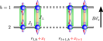
Figure 1: Spin-phonon coupled ladder model. Red arrows: spin-1/2 moments located at equilibrium positions $r_{l,h}$ on legs $h=1,2$ with longitudinal displacements $x_{l}$ independent of $h$. Dashed leg section: finite longitudinal phonon amplitude $\Delta x_{l}=x_{l}-x_{l+1}\neq 0$. AFM exchange $J_{\parallel(\perp)}$ on black legs (orange rungs). Green rectangles: rung singlet formation. Spin ’directions’: AFM nn-correlations. $B\vec{e}_{z}$: external magnetic field.

Quite recently the theory of spin-phonon drag has been revisited within a generic two-component model of interacting bosons Gangadharaiah2010a . Within this work, the formal equivalence of two distinct approaches for the description of drag, namely quasiclassical Boltzmann transport theory and Kubo linear response formalism, has been laid out, including several qualitative conclusions. However, a direct application of the ideas put forward to a more realistic situation is still lacking. Therefore, in this work we move ahead and study the spin-phonon drag in a spin-ladder coupled to acoustic phonons. One of our main conclusions is, that for magnetoelastic coupling strengths typical for cuprate ladders such as (La,Ca,Sr)₁₄Cu₂₄O₄₁, the drag conductivity can be of similar magnitude as the magnetic thermal conductivity and moreover displays a remarkably similar high-temperature dependence.

The outline of this paper is as follows. In section II we describe our model of a two-leg ladder coupled to lattice degrees of freedom. The spin dynamics of the ladder is treated in the limit of strong rung coupling, for which we resort to a bond-operator treatment in subsection II.2. The spin-phonon coupling is discussed in subsection II.3. In section III we detail our evaluation of the drag rates, for which we extend the approach of ref. Gangadharaiah2010a , by embedding its findings within the time convolutionless projection operator method to obtain the transport rates. In section IV we apply our approach to the specific case of (La,Ca,Sr)₁₄Cu₂₄O₄₁ ladders, contrasting the drag to the diagonal conductivities versus temperature and spin-phonon coupling strength as well as external magnetic fields. We conclude in section V.

II Spin-Phonon coupled Ladder

For the remainder of this study we focus on the two-leg spin-1/2 ladder depicted in Fig. 1 with magnetoelastic coupling of the spin degrees of freedom to lattice vibrations

$$H=H_{S}+H_{P}+H_{SP}\,,$$ (1)

where $H_{S,P,SP}$ refers to the spin, phonon, and spin-phonon parts of the total Hamiltonian $H$.

II.1 Lattice Dynamics of the Ladder

To keep the analysis simple, we refrain from any detailed modeling of 3D phonon spectra of ladder structures. Rather we assume a spin ladder with strong coupling across the rungs, both structurally as well as electronically. In turn intra-rung vibrations are discarded and we consider only longitudinal inter-rung vibration along the direction of the legs of the ladder as in Fig. 1. In turn $H_{P}$ refers to a single one-dimensional acoustic phonon

$$H_{P}=\sum_{q}\omega_{q}b_{q}^{\dagger}b_{q}^{\phantom{\dagger}}\,,$$ (2)

where $\omega_{q}{=}\omega_{D}|\text{sin}\left(q/2\right)|$ is the dispersion of the rung phonon $b_{q,h}^{(\dagger)}$ with a Debye energy $\omega_{D}$ and $q\in[-\pi,\pi[$. Several comments are in order regarding this phonon spectrum. First, we stress that other than for simplicity of later numerical calculations, the formal developments of our analysis do not depend on the phonon’s dimensionality. The latter primarily affects the low-temperature form of the phononic heat conduction for $T\ll\omega_{D}$, where it is sensitive to various scattering mechanism Klemens1951 ; Callaway1961 . However, we will be concerned primarily with the overall behavior of the thermal conductivity on temperature scales larger than the Debye energy, where the heat conduction of the pure phonon system is dominated by a constant specific heat and a scattering rate which increases proportional to the phonon density, i.e. $\propto T$, independent of dimension.

II.2 Spin Dynamics of the static Ladder

The spin Hamiltonian of the static ladder reads

$$H_{S}{=}\sum_{l}[J_{\perp}\vec{S}_{l,1}{\cdot}\vec{S}_{l,2}+\sum_{h=1,2}(J_{\parallel}\vec{S}_{l,h}{\cdot}\vec{S}_{l+1,h}{-}BS_{l,h}^{z})]\,$$ (3)

with intra(inter)-rung AFM exchange $J_{\perp(\parallel)}$, external magnetic field $B$, and periodic boundary conditions (PBC). To describe the spin excitations of the two-leg ladder for $B=0$ we use the well established bond-operator representation jurecka01 ; sachdev90 of dimerized spin-$1/2$ systems. Here we briefly recapitulate this method. The eigenstates of the total spin on a single rung are one singlet and three triplets. These can be created by the bosonic bond operators $s_{n}^{\dagger}$ and $t_{\alpha}^{\dagger}$ with $\alpha=x,y,z$ acting on a vacuum $|0\rangle$ by

$$s_{n}^{\dagger}|0\rangle = \frac{1}{\sqrt{2}}\left(|\uparrow\downarrow\rangle-|\downarrow\uparrow\rangle\right)_{n}$$

$$t_{x,n}^{\dagger}|0\rangle = -\frac{1}{\sqrt{2}}\left(|\uparrow\uparrow\rangle-|\downarrow\downarrow\rangle\right)_{n}$$

$$t_{y,n}^{\dagger}|0\rangle = \frac{i}{\sqrt{2}}\left(|\uparrow\uparrow\rangle+|\downarrow\downarrow\rangle\right)_{n}$$

$$t_{z,n}^{\dagger}|0\rangle = \frac{1}{\sqrt{2}}\left(|\uparrow\downarrow\rangle+|\downarrow\uparrow\rangle\right)_{n},$$ (4)

where the first (second) entry in the kets refers to site $1$($2$) of the rung $n$ of Fig. 1. On each site we have $[s,s_{\phantom{\alpha}}^{\dagger}]{=}1$, $[s_{\phantom{\alpha}}^{(\dagger)},t_{\alpha}^{(\dagger)}]{=}0$, and $[t_{\alpha}^{\phantom{(\dagger)}},t_{\beta}^{\dagger}]{=}\delta_{\alpha\beta}$. The bosonic Hilbert space has to be restricted to either one singlet or one triplet per site by the constraint

$$s_{n}^{\dagger}s_{n}^{\phantom{\dagger}}+t_{\alpha,n}^{\dagger}t_{n,\alpha}^{\phantom{\dagger}}=1.$$ (5)

Expressing $H_{S}$ by the bond operators yields a bose gas of singlets and triplets with two-particle interactions mediated by the inter-rung coupling $J_{\parallel}$. At $J_{\parallel}{=}0$ these interactions vanish leaving a sum of purely local rung Hamiltonians, which lead to a product ground-state of singlets localized on the rungs and a set of $3^{N}$-fold degenerate triplets. For finite $J_{\parallel}$ the inter-rung interactions can be treated approximately by a linearized Holstein-Primakoff (LHP) approach jurecka01 ; Chubokov89a ; chubukov91 ; Starykh96a ; brenig98 . The LHP method retains spin-rotational invariance and reduces $H_{S}$ to a set of three degenerate massive magnons (triplons)

$$H_{S}=\sum_{k}\Omega_{k}a_{\alpha,k}^{\dagger}a_{\alpha,k}^{\phantom{\dagger}}+\mbox{const.}$$ (6)

with

$$t_{\alpha,k}^{\dagger} = u_{k}a_{\alpha,k}^{\dagger}+v_{k}a_{\alpha,-k}^{\phantom{\dagger}},$$ (7)

$$\Omega_{k} = J_{\perp}\sqrt{1+2e_{k}}$$ (8)

$$e_{k} = \frac{J_{\parallel}}{J_{\perp}}\cos(k)$$ (9)

$$u[v]_{k}^{2} = \frac{1}{2}\left(\frac{J_{\perp}(1+e_{k})}{\omega_{k}}+[-]1\right).$$ (10)

The ’$[]$’-bracketed sign on the rhs. in (10) refers to the quantity $v$ on the lhs.. The spin-gap $\Delta{=}\min\{\Omega_{k}\}$ resides at $k{=}\pi$ with $\Delta{=}\sqrt{J_{\perp}^{2}-2J_{\perp}J_{\parallel}}$. Note that because of (7) the ground state $|D\rangle$, which is defined by $a_{\alpha,k}|D\rangle{=}0$, contains quantum-fluctuations beyond the pure singlet product-state. To leading order the dispersion $\Omega_{k}$ is identical to perturbative expansions Barnes93 ; Reigrotzki94 . Beyond the LHP approach triplet interactions and more elaborate consideration of the constraint (5) lead to a renormalization of $\Omega_{k}$ and the formation of multi-magnon bound states jurecka00-2 ; Kotov98 ; Kotov98-2 ; Kotov99 ; jurecka01-2 . However, for $J_{\parallel}\ll J_{\perp}$ - which we assume for the remainder of this work - these renormalizations can be neglected.

To keep $H_{S}$ diagonal at finite magnetic fields $B$ along the $z$-direction, we have to transform the $x,y,z$-spin projections of the triplets onto magnetic $z$-quantum numbers $m{=}\pm 1,0$ as usual

$$a_{x\{y\},k}^{\dagger}=\frac{1\{i\}}{\sqrt{2}}(a_{1,k}^{\dagger}+\{-\}a_{-1,k}^{\dagger})\,,\hphantom{a}a_{z,k}^{\dagger}=a_{0,k}^{\dagger}\,,$$ (11)

leading to the final spin Hamiltonian

$$H_{S}=\sum_{m,k}\Omega_{m,k}a_{m,k}^{\dagger}a_{m,k}\,,$$ (12)

with the dispersion

$$\Omega_{m,k}=\Omega_{k}+mB\,,$$ (13)

which splits into three non-degenerate branches at $B\neq 0$, according to the Zeeman energy.

II.3 Spin-Phonon Coupling

The central ingredient to the spin-phonon drag is some type of coupling between the triplon and phonon bath. Our work is based on a direct magnetoelastic coupling along the legs of the ladder. In fact from Fig. 1 we read off, that the on-leg exchange is subject to inhomogeneous deviations of the center of mass coordinate of the dimers from their equilibrium positions by

$$J_{||,l,l+1}=J_{\parallel}+\xi\Delta x_{l}\,,$$ (14)

where $\xi=-\partial J_{||}/\partial a$ with the on-leg lattice constant $a$, $\Delta x_{l}=(x_{l}-x_{l+1})$, and $\xi$ will usually be positive. Models for the super-exchange in cuprates Aronson1991 ; Cooper1990 ; Sulewski1990 ; Kawada1998 suggest a rather material sensitive range of possible values for $\xi$, with typically $J_{\parallel}\propto a^{-4}$. From (14) the spin-phonon part of (1) follows from its classical version regarding the deviations

$$H_{SP}=\sum_{l,h}\xi\Delta x_{l}\vec{S}_{l,h}{\cdot}\vec{S}_{l+1,h}$$ (15)

by quantizing the deviations

$$x_{q,h}=\sqrt{\frac{\hbar}{2M\omega_{q}}}(b_{-q}^{\dagger}+b_{q})$$ (16)

in terms of the phonons from subsection II.1 with the Fourier transform $x_{l}=\sum_{q}e^{iql}x_{q}/\sqrt{N}$.

After some algebra, expressing the spin operators in (15) completely analogous to those in (3) by bond bosons, using again the LHP approach and dropping all triplon vertices of order higher than quadratic, we arrive at an expression for $H_{SP}$ in terms of two-triplon-one-phonon vertices

$$H_{SP}=\sum_{k,q,m,h}(b_{-q,h}^{\dagger}+b_{q,h})\left[\Gamma_{k,q}^{\text{an}}(a_{-m,-k}^{\dagger}a_{m,k+q}^{\dagger}+\right.$$ (17)

$$\left.\hphantom{aaaaaaa}a_{-m,k}a_{m,-k-q})+\Gamma_{k,q}^{\text{n}}\,a_{m,k+q}^{\dagger}a_{m,k}\right]\hphantom{aaa}$$

with

$$\Gamma_{k,q}^{\text{an}} = -i\,\gamma_{k,q}\,e^{-i(k+(q/2))}$$ (18)

$$\Gamma_{k,q}^{\text{n}} = -2i\,\gamma_{k,q}\,\text{cos}(k+(q/2))$$ (19)

$$\gamma_{k,q} = \frac{g(u_{k}+v_{k})(u_{k+q}+v_{k+q})\text{sin}(\frac{q}{2})}{\sqrt{N|\text{sin}(\frac{q}{2})|}}$$ (20)

and the coupling constant

$$g=\sqrt{\frac{\hbar^{2}}{2M\omega_{D}}}\xi\,.$$ (21)

We have used $\omega_{q}=\omega_{-q}$. Note that both $\Gamma_{k,q}^{\text{n}}$ and $\Gamma_{k,q}^{\text{an}}$ do not depend on the magnetic quantum number $m$. The scattering processes in (17) featuring $\Gamma_{k,q}^{\text{n}}$ correspond to processes where a magnon is scattered under creation or annihilation of a phonon, the magnon conserves its magnetic quantum number. These processes will be called normal processes in the following. Terms with $\Gamma_{k,q}^{\text{an}}$ correspond either to processes, where two magnons of opposite magnetic quantum number are created (annihilated) along with the annihilation (creation) of a phonon, or to processes where two magnons of opposite magnetic quantum number and one phonon are simultaneously created (annihilated). The former will be called anomalous processes and the latter processes (vacuum fluctuations) are irrelevant for transport.

Next we briefly discuss some very rough orders of magnitude for the spin-phonon scattering in cuprate ladders. First, in those materials $J_{\parallel(\perp)}{\gg}\omega_{D}$. Second, both normal and anomalous processes give rise to final states with at least one triplon, i.e., the final DOS is at most $O(1/J_{\parallel}).$ Therefore the parameter driving perturbation theory is $|g/J_{\parallel}|$. Using (21) we get $|g/J_{\parallel}|=|(\partial J_{\parallel}/\partial a)(a/J_{\parallel})|/\sqrt{(M/m)(2ma^{2}/\hbar^{2})(\omega_{D})}$ where we have inserted the free electron mass $m$. For the longitudinal type of dimer phonon, Fig. 1, $M$ refers to some total mass of two copper and eight oxygen atoms, i.e., $M/m\sim O(10^{5})$. For typical cuprate lattice spacings of $a\sim 4\text{\AA}$ one has $\hbar^{2}/(2ma^{2})\sim O(100meV)$, and finally $\omega_{D}\sim O(10meV)$. This yields $|g/J_{\parallel}|=|(\partial J/\partial a)(a/J)|/O(10^{2})$. With $J\propto a^{-n}$, cf. ref.Aronson1991 ; Cooper1990 ; Sulewski1990 ; Kawada1998 , it follows that $|g/J_{\parallel}|=O(n/100)$. From $n\sim 2\ldots 4$, and given the very approximate nature of the preceding argument, one may expect $|g/J_{\parallel}|\sim O(10^{-2})\ldots O(10^{-1})$, which also implies that perturbation theory in terms of $g$ for the coupled spin-phonon system is well justified.

III Thermal Transport and Drag

III.1 Scattering Rates

Now we analyze the transport relaxation rates relevant for a Boltzmann description of the mutual current drag in the coupled spin-phonon system of the preceding section. Deriving drag rates is not a settled issue and different routes may be pursued. Direct evaluation of collision terms have been shown to agree with results from diagrammatic calculations of the linear-response conductivities Gangadharaiah2010a . Memory functions form another powerful approach Boulat2007a . Here we consider yet an alternative construction of drag rates following a recent study of electron-phonon coupling in 1D atomic wires Bartsch2011a . Within this construction the time convolutionless (TCL) projection operator method TCL1 ; TCL2 ; TCL3 is employed to reduce the quantum dynamics of deviations of occupation numbers in momentum space from their equilibrium values to a set of rate equations. The later rates can be interpreted in terms of collision rates of the linearized Boltzmann equation Bartsch2010a . While in ref. Bartsch2011a this approach has been used for the diagonal collision rates of a mixed fermion-boson system, here we will focus on the off-diagonal rates, which describe the drag in a two-component boson-boson system.

For completeness we summarize the main ingredients of the TCL projection operator method. Given any decomposition of the Hamiltonian $H=H_{0}+V$, the TCL approach is a perturbative scheme to derive a closed system of equations of motion for a set of ’relevant’ quantities TCL1 ; TCL2 ; TCL3 . In our case the perturbation $V$ refers to the magnon-phonon-coupling and perturbation theory is applicable in the spirit of the last paragraph of section II.3, i.e., $g^{2}/J_{\parallel}\ll J_{\parallel},\omega_{D}$. The main idea is to define a projection operator $\mathcal{P}$ which maps the system’s complete time-dependent density matrix $\rho(t)$ onto a reduced density matrix-like object $\mathcal{P}\rho(t)$ which only incorporates the dynamics of the relevant variables.

As detailed in Bartsch2010a , a proper construction of the projection operator ${\cal P}$ involves ’coarse graining’ of momentum space. Observable transport processes will be independent of a particular choice of the graining in the limit of small grain size. Different types of graining have been discussed in Bartsch2010a ; Bartsch2011a . For the present model, one starts off from the deviation of the triplon (phonon) density at fixed momentum $k$ ($q$) from equilibrium, i.e. $\Delta_{m,k}^{\text{S}}=a_{m,k}^{\dagger}a_{m,k}-g_{m,k}$ ($\Delta_{q}^{\text{P}}=b_{q}^{\dagger}b_{q}-p_{q}$), where $g_{m,k}$ ($p_{q}$) are the triplon (phonon) equilibrium Bose distributions. Using this, the operators

$$D_{m,\kappa}^{\text{S}}=\sum_{k\in\kappa}\frac{\rho^{eq}\Delta_{m,k}^{\text{S}}}{\text{Tr}[\rho^{eq}\Delta_{m,k}^{\mathrm{S}\,2}]},\quad D_{\eta}^{\text{P}}=\sum_{q\in\eta}\frac{\rho^{eq}\Delta_{q}^{\text{P}}}{\text{Tr}[\rho^{eq}\Delta_{q}^{\mathrm{P}\,2}]}$$ (22)

are introduced, where the Greek index $\kappa$ ($\eta$) labels a grain in the magnon’s (phonon’s) momentum space and $\rho^{\mathrm{eq}}$ corresponds to the equilibrium density matrix, i.e., $\text{Tr}[\rho^{\mathrm{eq}}a_{m,k}^{\dagger}a_{m,k}]=g_{m,k}$ and $\text{Tr}[\rho^{\mathrm{eq}}b_{q}^{\dagger}b_{q}]=p_{q}$. From eqn. (22), the projected density matrix is defined

$$\mathcal{P}\rho(t)=\rho^{\mathrm{eq}}+\sum_{m,\kappa}\frac{D_{m,\kappa}^{\text{S}}d_{m,\kappa}^{\text{S}}(t)}{N_{m,\kappa}}+\sum_{\eta}\frac{D_{\eta}^{\text{P}}d_{\eta}^{\text{P}}(t)}{N_{\eta}}\,,$$ (23)

where $N_{m,\kappa}$ ($N_{\eta}$) are the number of states per grain and $d_{m,\kappa}^{\text{S}}(t)$ ($d_{\eta}^{\text{P}}(t)$) are the on-grain density deviations

$$\begin{array}[]{lcl}d_{m,\kappa}^{\text{S}}(t)=\text{Tr}[\Delta_{m,\kappa}^{\text{S}}\rho(t)]&&d_{\eta}^{\text{P}}(t)=\text{Tr}[\Delta_{\eta}^{\text{P}}\rho(t)]\\ \\ \Delta_{m,\kappa}^{\text{S}}=\sum_{k\in\kappa}\Delta_{m,k}^{\text{S}}&&\Delta_{\eta}^{\text{P}}=\sum_{q\in\eta}\Delta_{q}^{\text{P}}.\end{array}$$ (24)

These density deviations form the set of relevant variables.

To leading order in $V$, i.e., $g$, and introducing the vector $\mathbf{d}(t)=(\mathbf{d}^{\textrm{S}}(t),\mathbf{d}^{\textrm{P}}(t))=(d_{m,\kappa}^{\text{S}}(t),d_{\eta}^{\text{P}}(t))$ of the relevant variables, the TCL projection approach now results in a system of rate equations which couples all magnon and phonon occupation number deviations as

$$\dot{\mathbf{d}}(t)=\mathbf{R}(t)\mathbf{d}(t),\quad\mathbf{R}(t)=\left[\begin{array}[]{ll}\mathbf{R}^{\text{S}}(t)&\mathbf{R}^{\text{P-S}}(t)\\ \mathbf{R}^{\text{S-P}}(t)&\mathbf{R}^{\text{P}}(t)\end{array}\right]\,.$$ (25)

The $2\times 2$ block-structured rate matrix allows for a direct interpretation in terms of momentum redistribution. While the diagonal blocks $\mathbf{R}^{\text{S(P)}}$ account for transitions between momentum grains within the triplon (phonon) sector of the Hilbert space due to the presence of phonons (triplons), the off-diagonal blocks $\mathbf{R}^{\text{P-S(S-P)}}$ quantify a momentum pickup of the phonons (triplons) from the triplons (phonons), i.e., mutual drag.

Analytic expressions for $\mathbf{R}^{\mathrm{S-P(P-S)}}$ to leading order in $g$ are evaluated in close analogy to Bartsch2010a ; Bartsch2011a . For the drag rates, and after some algebra, we get

$$R_{\eta,(m,\kappa)}^{\text{S-P}}(t)=\sum_{i\in\kappa,j\in\eta}\frac{2}{\hbar^{2}N_{m,\kappa}}\int_{0}^{t}\text{d}\tau$$

$$\left[|\Gamma_{i,-j}^{\text{n}}|^{2}(1{+}g_{m,i-j}{+}p_{m,j})\text{cos}(\frac{\varepsilon_{m,i}{-}\varepsilon_{m,i-j}{-}\omega_{j}}{\hbar}\tau)\right.$$

$$+|\Gamma_{i,j}^{\text{n}}|^{2}(g_{m,i+j}{-}p_{j})\text{cos}(\frac{\varepsilon_{m,i}{-}\varepsilon_{m,i+j}{+}\omega_{j}}{\hbar}\tau)$$

$$+4|\Gamma_{i,-j}^{\text{an}}|^{2}(g_{-m,j-i}{-}p_{j})\text{cos}(\frac{\varepsilon_{m,i}{+}\varepsilon_{-m,j-i}{-}\omega_{j}}{\hbar}\tau)$$

$$\left.+4|\Gamma_{i,j}^{\text{an}}|^{2}(1{+}g_{-m,-i-j}{+}p_{j})\text{cos}(\frac{\varepsilon_{m,i}{+}\varepsilon_{-m,-i-j}{+}\omega_{j}}{\hbar}\tau\right]$$

and

$$R_{(m,\eta),\kappa}^{\text{P-S}}(t)=\sum_{i\in\kappa,j\in\eta}\frac{2}{\hbar^{2}N_{\kappa}}\int_{0}^{t}\text{d}\tau$$

$$\left[|\Gamma_{j,-i}^{\text{n}}|^{2}(g_{m,j-i}{-}g_{m,j})\text{cos}(\frac{\varepsilon_{m,j}{-}\varepsilon_{m,j-i}{-}\omega_{i}}{\hbar}\tau)\right.$$

$$+|\Gamma_{j,i}^{\text{n}}|^{2}(g_{m,i+j}{-}g_{m,j})\text{cos}(\frac{\varepsilon_{m,j}{-}\varepsilon_{m,j+i}{+}\omega_{i}}{\hbar}\tau)$$

$$+4|\Gamma_{j,-i}^{\text{an}}|^{2}(1{+}g_{-m,i-j}{+}g_{m,j})\text{cos}(\frac{\varepsilon_{m,j}{+}\varepsilon_{-m,i-j}{-}\omega_{i}}{\hbar}\tau)$$

$$\left.+4|\Gamma_{j,i}^{\text{an}}|^{2}(1{+}g_{-m,-i-j}{+}g_{m,j})\text{cos}(\frac{\varepsilon_{m,j}{+}\varepsilon_{-m,-i-j}{+}\omega_{i}}{\hbar}\tau)\right].$$

Note that these expressions are valid at all times. Only in the long-time limit they will display the familiar ’energy-conserving’ $\delta$-functions. In each of (III.1) and (III.1), the first two rate terms result from normal processes and the remaining two from anomalous processes, where the last one corresponds to a simultaneous creation (annihilation) of two magnons and one phonon and is forbidden in the long-time limit because of energy conservation.

For the diagonal rates $\mathbf{R}^{\mathrm{S(P)}}$, expressions similar to (III.1,III.1) can be derived in principle. However, for the remainder of this paper we will follow a different route. Namely, in addition to the triplon-phonon scattering, we will include all other potentially relevant diagonal relaxation mechanisms not contained in our model on a phenomenological basis. This includes impurity scattering, triplon-triplon interactions beyond eqn. (6), and phonon anharmonicities. We assume these rates to be diagonal $R_{(m,\kappa),(n,\eta)}^{\text{S}}{\approx}-\delta_{\kappa\eta}\delta_{mn}/\tau_{m,\kappa}^{\text{S}}$ and $R_{k,i}^{\text{P}}{\approx}-\delta_{\kappa\eta}/\tau_{\kappa}^{\text{P}}$, with relaxation times $\tau_{m,\kappa}^{\text{S}}$ and $\tau_{\eta}^{\text{P}}$ which may still depend on temperature, the momentum grain index, as well as the triplon’s magnetic quantum number.

III.2 Thermal Conductivity

Following the standard Chapman-Enskog procedure Jaeckle1978 we now set up the linearized Boltzmann equation. To that end we introduce additional ’vectors’

$$\mathbf{n}=(g_{m,\kappa},p_{\eta})\hphantom{aaaaa}\textrm{equilibrium distributions}\hphantom{\,,}$$

$$\boldsymbol{\varepsilon}=(\varepsilon_{m,\kappa},\omega_{\eta})\hphantom{aaaaaaaaaaaaaaaaaaa}\textrm{energies}\hphantom{\,,}$$

$$\mathbf{v}=(\partial_{k}\varepsilon_{m,\kappa},\partial_{k}\omega_{\eta})=(v_{m,\kappa},u_{\eta})\hphantom{aa.a}\textrm{velocities}\,,$$ (28)

using the triplon and phonon subsystem indices $m,\kappa$ and $\eta$. To simplify notations, the triplon indices will also be subsumed into a single Greek letter $\xi$. For slow spatial and time variations, i.e., in the hydrodynamic regime, and to leading order, the Chapman-Enskog expansion links the change of the distribution function to its deviation from equilibrium via the rates of eqn. (25) by

$$-\frac{\partial n_{\alpha}}{\partial\varepsilon}\frac{\varepsilon_{\alpha}}{T}\left(\mathrm{v}_{\alpha}\partial_{x}T\right)=\sum_{\beta}R_{\alpha\beta}d_{\beta}\,.$$ (29)

Since the heat current density is $\vec{j}=\frac{1}{Ga}\sum_{\alpha}\varepsilon_{\alpha}\vec{\mathrm{v}}_{\alpha}d_{\alpha}$, where $G$ corresponds to the number of grains and $a$ is the lattice constant, the thermal conductivity follows from (29) as

$$\kappa=\frac{1}{GaT}\sum_{\alpha,\beta}\mathrm{v}_{\alpha}\varepsilon_{\alpha}R_{\alpha\beta}^{-1}\varepsilon_{\beta}\mathrm{v}_{\beta}\frac{\partial n_{\beta}}{\partial\varepsilon}\,$$ (30)

with the $2\times 2$-block inverse collision term matrix $R_{\alpha\beta}^{-1}$. In turn the thermal conductivity decomposes into four parts

$$\kappa=\kappa_{\text{S}}+\kappa_{\text{P}}+\kappa_{\text{P-S}}+\kappa_{\text{S-P}}\,,$$ (31)

which can be identified as the conventional magnon and phonon conductivities $\kappa_{\text{S}}$, $\kappa_{\text{P}}$, which are diagonal, i.e., $\kappa=\eta$, and two drag conductivities $\kappa_{\text{P-S}}$, $\kappa_{\text{S-P}}$, which are off-diagonal, i.e., $\kappa\neq\eta$. Assuming that $R^{\text{S}}$, $R^{\text{P}}$ $\gg$ $R^{\text{S-P}}$, $R^{\text{P-S}}$, the inverse collision term simplifies, and we obtain the usual diagonal conductivities

$$\kappa_{\text{S}} = -\frac{1}{Ga}\frac{1}{T}\sum_{\xi}v_{\xi}^{2}\varepsilon_{\xi}^{2}\tau_{\xi}^{\text{S}}\frac{\partial g_{\xi}}{\partial\varepsilon}$$

$$\kappa_{\text{P}} = -\frac{1}{Ga}\frac{1}{T}\sum_{\eta}u_{\eta}^{2}\omega_{\eta}^{2}\tau_{\eta}^{\text{P}}\frac{\partial p_{\eta}}{\partial\omega}\,,$$ (32)

where $\xi$ ($\eta$) runs over the triplon (phonon) grains only. The drag conductivities read

$$\kappa_{\text{S-P}} = -\frac{1}{Ga}\frac{1}{T}\sum_{\eta,\xi}(v_{\xi}\varepsilon_{\xi}\tau_{\xi}^{\text{S}})(u_{\eta}\omega_{\eta}\tau_{\eta}^{\text{P}})\frac{\partial g_{\xi}}{\partial\varepsilon}R_{\eta,\xi}^{\text{S-P}}$$

$$\kappa_{\text{P-S}} = -\frac{1}{Ga}\frac{1}{T}\sum_{\xi,\kappa}(v_{\xi}\varepsilon_{\xi}\tau_{\xi}^{\text{S}})(u_{\kappa}\omega_{\kappa}\tau_{\kappa}^{\text{P}})\frac{\partial p_{\kappa}}{\partial\omega}R_{\xi,\kappa}^{\text{P-S}}.\,\,\,\,\,\,\,\,\,\,\,\,\,$$ (33)

Using eqns. (III.1,III.1), and after some algebra one can show that $\kappa_{\text{S-P}}=\kappa_{\text{P-S}}\equiv\kappa_{\text{D}}$/2. As a consistency check, we note that eqns. (33) are identical to those derived in ref. Gangadharaiah2010a , using however different methods.

IV Application to Cuprate Ladders

In this section we will perform a numerical evaluation of (III.1,III.1) and (32,33), to provide a semi quantitative estimate of the size of the drag as compared to the diagonal conductivities using a set of parameters which might be of relevance to the cuprate spin ladder La₅Ca₉Cu₂₄O₄₁ (LCCO) Hess2001a ; Hess2005a ; Hess2006a ; Otter2012a .

For the remainder of this work we will assume the diagonal scattering times to be temperature dependent but momentum independent. First we consider reduced quantities $G_{\text{S,P,D}}$ for the conductivities of the triplons, phonons, and drag. These are obtained by stripping $\kappa_{\text{S,P,D}}$ from their dependence on the diagonal scattering times $\tau^{\text{S(P)}}$ and the scale of the spin-phonon drag time $\tau^{\text{D}}$

$$G_{\text{S(P)}}=\frac{\kappa_{\text{S(P)}}}{\tau^{\text{S(P)}}}\,,\hphantom{aaa}G_{\text{D}}=\frac{\tau^{\text{D}}\kappa_{\text{D}}}{\tau^{\text{S}}\tau^{\text{P}}}\,,\hphantom{aaa}\tau^{\text{D}}\equiv\frac{\hbar J_{\parallel}}{g^{2}}\,.$$ (34)

These reduced quantities allow to compare the relative size of the various conductivities versus temperature $T$ and magnetic field $B$, independent of their mean-free paths and involve the parameters $J_{\parallel}$ and $\omega_{D}$ only. Using $J_{\perp}\approx\text{k}_{\text{b}}\,1200\,\text{K}$ Hess2001a ; Hess2005a ; Hess2006a ; Otter2012a , the former is set to $J_{\parallel}=0.45J_{\perp}$, which approximately captures the spin gap $\Delta_{T}$ of the LCCO ladders which is $\Delta_{T}\approx\text{k}_{\text{b}}\,380\,\text{K}$. For the phonons we chose a Debye energy of $\omega_{\text{D}}\approx 0.32J_{\perp}$. For these parameters only the normal processes in eqn. (17) contribute to the scattering rates in eqns. (III.1,III.1). Finally, only the long-time limit of the latter equations will be used in the following discussion.

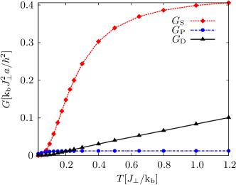
Figure 2: Reduced thermal conductivities $G_{\text{S}}$, $G_{\text{P}}$ and $G_{\text{D}}$ from eqn. (34) versus temperature at $B=0$. The drag contribution $G_{\text{D}}$ is of the same order of magnitude as $G_{\text{S}}$. While $G_{\text{S}}$ and $G_{\text{P}}$ become constant for large $T$, $G_{\text{D}}$ grows linearly in this limit. Parameters: $J_{\parallel}=0.45J_{\perp}$, i.e., gap $\approx 0.3J_{\perp}$ for $B=0$, $\omega_{D}\approx 0.3\,J_{\perp},N=400$.

Fig. 2 displays $G_{\text{S,P,D}}$ versus temperature at $B=0$. For the numerical evaluation we have checked, that the results are independent of the coarse graining procedure in the limit of small grains and we have chosen system sizes, typically $N=400$ rungs, such that finite size effects remain negligible on the scale of plots discussed in the following. Fig. 2 shows that the ratio between the reduced triplon and drag conductivities is of $O(10)$ for typical temperatures within the range depicted. With eqn. (34), this implies, that for the triplon and drag conductivities to be of comparable size, $g^{2}\tau^{\text{P}}/(\hbar J_{\parallel})\sim O(10)$ should hold. As we will show later, this is not unrealistic for LCCO. The temperature dependence of $G_{\text{S}}$ and $G_{\text{P}}$ is as expected, i.e., at $T\ll J$, $G_{\text{S}}$ shows exponential Arrhenius behavior, while $G_{\text{P}}$ increases linearly for $T\ll\omega_{D}$ due to the $1$D phonon dispersion. The latter is only visible for the very low temperature scales of Fig. 2. For $T\gg J$ and $\omega_{D}$, both quantities $G_{\text{S}}$ and $G_{\text{P}}$ saturate. $G_{\text{D}}$, on the other hand, increases linearly with $T$ in the intermediate and high temperature range depicted. This is an effect, arising from the combined high-temperature behavior of the sums of Bose functions in both drag rates (III.1,III.1), and the derivatives $(\partial g/\partial\varepsilon)$ and $(\partial p/\partial\omega)$ in (33).

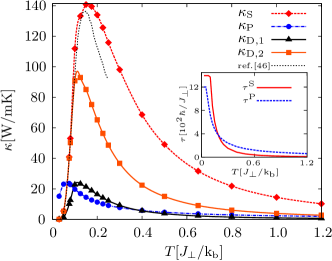
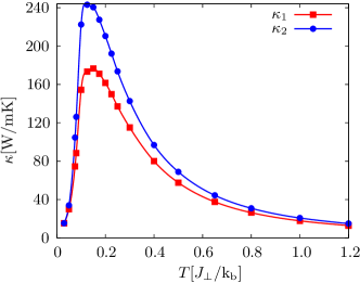
Figure 3: (a) Temperature dependence of thermal conductivities $\kappa_{\text{S}}$ (checks) and $\kappa_{\text{P}}$ (dots) (32) as well as of $\kappa_{\text{D}}$ (33) for $g=0.1J_{\parallel}$ (triangles) and $g=0.2J_{\parallel}$ (squares) without magnetic field $B$. Dashed line without symbols: experimental data for spin heat conductivity in LCCO from ref.Hess2005a . $\kappa_{\text{D}}$ is of the same order of magnitude as $\kappa_{\text{S}}$. The maximum for $\kappa_{\text{D}}$ lies at lower temperatures than for $\kappa_{\text{S}}$. Inset: Dependence of relaxation times $\tau^{\text{S}}$ (solid) and $\tau^{\text{P}}$ (dotted) in $[10^{2}\hbar/J_{\perp}]$ on $T$ in $[J_{\perp}/\text{k}_{\text{b}}]$ Parameters: $J_{\perp}=\text{k}_{\text{b}}1200\,\text{K}$, $J_{\parallel}=0.45J_{\perp}$ (i.e., gap $\approx 0.3J_{\perp}$ for $B=0$), $\omega_{D}\approx 0.3\,J_{\perp}$, $a=4\cdot 10^{-10}\ \text{m},N=400$. (b) Total conductivity $\kappa_{\text{S}}+\kappa_{\text{P}}+\kappa_{\text{D}}$ for $g=0.1J_{\parallel}$ ($\kappa_{1}$) and $g=0.2J_{\parallel}$ ($\kappa_{2}$).

To evaluate the thermal conductivities semi-quantitatively we have to fix the parameters $g$, $\tau^{\text{S}}$ and $\tau^{\text{P}}$. The diagonal scattering times $\tau^{\text{S}}$ and $\tau^{\text{P}}$ are chosen to approximately account for the known transport data of LCCO, discarding any drag contribution a priori. To this end we assume that the low-temperature scattering for phonons and triplons can be expressed by a temperature-independent effective mean free path $l_{\text{P(S)}}^{0}$ resulting from grain-boundaries, impurities etc.. The relation between the mean free paths and the scattering times is set to $\tau^{\text{P(S)}}(T)=l_{\text{P(S)}}(T)/v_{\text{P(S}\text{),max}}$, where $v_{\text{P(S)},\text{max}}$ is the maximum phonon(triplon) group velocity. At high temperatures the diagonal mean free paths are assumed to be determined by scattering from a bosonic bath, which may either stem from phonons or triplons. This suggests an expansion of the mean free path as $l_{\text{P(S)}}^{T}=a_{\text{P(S)}}/T+b_{\text{P(S)}}/T^{2}+\ldots$ Alvarez2002a . Altogether we have $l_{\text{P(S)}}(T)=\mathrm{min}(l_{\text{P(S)}}^{0},l_{\text{P(S)}}^{T})$. To mimic the experimental data, existing for LCCO for temperatures $T\lesssim 300\,\text{K}$ Hess2001a ; Hess2005a ; Hess2006a ; Hess2007a ; Alvarez2002a , we found that $l_{\text{P}}^{0}\approx 770\text{\AA}$, $a_{\text{P}}\approx 55.3\cdot 10^{3}\text{\AA}\text{K}$, and $b_{\text{P}}\approx 0$ for the phonons and $l_{\text{S}}^{0}\approx 2960\text{\AA}$, $a_{\text{S}}\approx 0$, and $b_{\text{S}}\approx 4.18\cdot 10^{7}\text{\AA}\text{K}^{2}$ is acceptable. We emphasize, that, while phonon relaxation mechanisms are rather well understood, the approximate form of the temperature dependence for $\tau^{\text{S}}$ merely serves as a fitting parameter, and in particular $a_{\text{S}}\approx 0$ may not apply for $T\gtrsim 300\,\text{K}$. However, this does not impair any of our following conclusions. Finally, to evaluate the bulk conductivity, we rescale our 1D theory by the perpendicular surface area $A\approx 35.6\text{\AA}^{2}$ per spin ladder.

Using the preceding scattering rates, Fig. 3 displays the diagonal conductivities versus temperature at zero magnetic field. The inset of Fig. 3 shows $\tau^{\text{P(S)}}$. First, and as a consequence of our choice of $\tau^{\text{P(S)}}$, the overall magnitude and peak location of $\kappa_{\text{S(P)}}$ agree roughly with experiment Hess2001a ; Hess2005a ; Hess2006a ; Hess2007a ; Alvarez2002a . Second, Fig. 3 depicts the drag conductivities, using the same $\tau^{\text{P(S)}}$, and two typical spin phonon coupling constants $g$=0.1 and 0.2$J_{\parallel}$. As discussed in section II.3, such values of $g$ are well within reach for cuprates. In turn, as one main point of this paper, Fig. 3 demonstrates, that for reasonable magnetoelastic coupling strengths, the magnitude of the drag conductivity may well be comparable with that of the diagonal triplon conductivity. Due to $\kappa_{D}\propto g^{2}$, more quantitative considerations will depend sensitively on material details, suggesting that existing interpretations of experimental data in terms of diagonal conductivities only may need to be reexamined.

Turning to the temperature dependence in Fig. 3, and following the discussion of $G_{\text{S,P,D}}$(T), we first note that $\kappa_{\text{D}}\propto T\tau^{\text{P}}\tau^{\text{S}}$ at high temperatures. Therefore, and as another main point of this paper, $\kappa_{\text{S}}$ and $\kappa_{\text{D}}$ behave asymptotically identical at high temperatures, where $\tau^{\text{P}}\propto 1/T$ is firmly established. This can been seen clearly in Fig. 3. I.e., the triplon and drag contributions to the high-temperature transport are entangled inseparably. Regarding low temperatures, $\kappa_{\text{S}}$ displays an Arrhenius-behavior, as expected from the spin gap. This behavior also translates into the drag. The low temperature phonon conductivity is $\propto T$. This is an artifact of our 1D phonon model.

Fig. 3 shows the total heat conductivity. Three comments are in order. First, and as a detail of our model parameters, this figure clarifies, that our choice for the Debye temperature and the size of the spin gap do not fully reflect the material specifics of LCCO, where the phonon peak is split off into the spin-gap Hess2001a . Second, and more important, this figure demonstrates that even in the case of strong drag, i.e., $g$=0.2, the drag does not lead to additional structures in the temperature dependence of the total conductivity. Finally, since our starting point has been a fit to the observed diagonal conductivities without considering drag, the magnitude of the total conductivity does not agree with experiment.

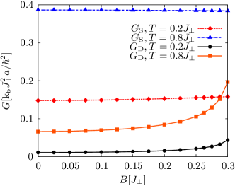
Figure 4: Reduced thermal conductivities $G_{\text{S}}$ and $G_{\text{D}}$ from eqn. (34) as a function of the magnetic field $B$ for a temperature smaller ($T=0.2J_{\perp}$) and a temperature larger ($T=0.8J_{\perp}$) than the spin gap. The drag contribution $G_{\text{D}}$ shows a significantly stronger $B$-dependence than $G_{\text{S}}$, especially for high temperatures. Parameters: $J_{\parallel}=0.45J_{\perp}$ (i.e., gap $\approx 0.3J_{\perp}$ for $B=0$), $\omega_{D}\approx 0.3\,J_{\perp},N=400$.

While the typical exchange energies in LCCO are too large to allow for sizeable manipulation of the triplon dispersion by experimentally accessible magnetic fields, it is nevertheless interesting to investigate also the field dependence of the reduced thermal conductivities $G_{\text{S}}$ and $G_{\text{D}}$. This may be relevant for appropriate low-$J_{\perp,\parallel}$ spin ladders as, e.g., in ref. Thielmann09a . The results are shown in Fig. 4 up to fields of $0.3J_{\perp}$, which almost close the spin gap for $J_{\parallel}=0.45J_{\perp}$, and for two temperatures $T=0.2J_{\perp}$ and $0.8J_{\perp}$, which are below and above the magnon gap. We note that $G_{\text{P}}$ is strictly field independent in our model. As is obvious from the figure, the diagonal triplon contribution is almost field independent for the temperatures depicted. This can be understood in terms of a near cancellation of the change in contributions to $\kappa_{\text{S}}$ from the $S^{z}=\pm 1$ triplon branches in finite fields. At significantly lower temperatures a weak field dependence of $G_{\text{S}}$ can be observed. In contrast to $G_{\text{S}}$, $G_{\text{D}}$ shows a clearly visible upward curvature versus $B$ for larger fields. This behavior increases with temperature. It is tempting to speculate, that such behavior may help to identify materials with sizeable drag contributions to their thermal conductivity.

V Conclusion

To summarize, we have investigated the spin-phonon drag effect in the thermal transport of two-leg spin ladders. Using a bond-operator description for the spin excitations and magnetoelastic coupling to longitudinal lattice vibrations we have employed the TCL projection operator method to map the quantum dynamics of the coupled spin and phonon system onto a linear Boltzmann equation from which an expression for the thermal conductivity has been obtained via the Chapman-Enskog approach. We have shown, that for magnetoelastic coupling strengths which are well within reach for cuprate spin ladders, the drag contribution to the total conductivity is not negligible, but rather can be of a size similar to that of the diagonal magnetic heat conductivity. Moreover, we have found, that the drag may be delicate to discriminate from the diagonal magnetic conductivity by means of the temperature dependence, since their high temperature behavior is asymptotically identical and at intermediate temperatures the drag does not lead to additional structures. Finally, we have pointed out, that finite magnetic fields may signal drag contributions to the conductivity. While the main conclusions of this work should be rather insensitive to details of the model parameters used in our numerical analysis, it seems highly desirable to enhance upon the ideas put forward here by considering a more realistic and 3D version of the phonon spectrum and the corresponding magnetoelastic coupling geometries.

- (1) A.V. Sologubenko, K. Gianno, H.R. Ott, U. Ammerahl, A. Revcolevschi, Phys. Rev. Lett. 84, 2714 (2000).
- (2) C. Hess, C. Baumann, U. Ammerahl, B. Büchner, F. Heidrich-Meisner, W. Brenig, and A. Revcolevschi, Phys. Rev. B 64, 184305 (2001).
- (3) K. Kudo, S. Ishikawa, T. Noji, T. Adachi, Y. Koike, K. Maki, S. Tsuji, K. Kumagai, J. Phys. Soc. Jpn. 70, 437 (2001).
- (4) A.V. Sologubenko, E. Felder, K. Gianno, H.R. Ott, A. Vietkine, A. Revcolevschi, Phys. Rev. B 62, R6108 (2000).
- (5) A.V. Sologubenko, K. Gianno, H.R. Ott, A. Vietkine, A. Revcolevschi, Phys. Rev. B 64, 054412 (2001).
- (6) C. Hess, H. ElHaes, A. Waske, B. Büchner, C. Sekar, G. Krabbes, F. Heidrich-Meisner, W. Brenig, Phys. Rev. Lett. 98, 027201 (2007).
- (7) C. Hess, Eur. Phys. J., Special Topics, 151, 73 (2007).
- (8) F. Heidrich-Meisner, A. Honecker, and W. Brenig, Eur. Phys. J. Special Topics 151, 135 (2007).
- (9) E. Shimshoni, N. Andrei, and A. Rosch, Phys. Rev. B 68, 104401 (2003).
- (10) A. V. Rozhkov and A. L. Chernyshev, Phys. Rev. Lett. 94, 087201 (2005).
- (11) A. L. Chernyshev and A. V. Rozhkov, Phys. Rev. B 72, 104423 (2005).
- (12) K. Louis, P. Prelovsek, and X. Zotos, Phys. Rev. B 74, 235118 (2006).
- (13) E. Gurevich and G. A. Roman, Sov. Phys. Solid State , 2102 (1967).
- (14) E. Boulat, P. Mehta, N. Andrei, E. Shimshoni, and A. Rosch, Phys. Rev. B 76, 214411 (2007).
- (15) A. L. Chernyshev, J. Magn. Magn. Mater. 310, 1263 (2007).
- (16) T. Holstein, Ann. Phys. 29, 410 (1964).
- (17) J. Bass, W. P. Pratt, and P. A. Schroeder, Rev. Mod. Phys. 62, 645 (1990).
- (18) L. Gurevich, J. Phys. (Moscow) 9, 477 (1945); 10, 67 (1946).
- (19) J. M. Ziman, Electrons and Phonon (Clarendon Press, Oxford, 1963).
- (20) S. Gangadharaiah, A. L. Chernyshev, and W. Brenig, Phys. Rev. B 82, 134421 (2010).
- (21) P. G. Klemens, Proc. R. Soc. Lond. A 208, 108 (1951)
- (22) J. Callaway, Phys. Rev. 113, 1046 (1995); ibid 122, 787 (1961).
- (23) C. Jurecka, W. Brenig, Phys. Rev. B 63, 094409 (2001).
- (24) S. Sachdev and R. N. Bhatt, Phys. Rev. B 41, 9323 (1990).
- (25) A. V. Chubukov, Pis’ma Zh. Eksp. Teor. 49, 108 (1989); [JETP Lett. 49, 129 (1989)].
- (26) A. V. Chubukov and Th. Jolicoeur, Phys. Rev. B 44, 12050 (1991).
- (27) O. A. Starykh, M. E. Zhitomirsky, D. I. Khomskii, R. R. P. Singh, and K. Ueda, Phys. Rev. Lett. 77, 2558 (1996).
- (28) W. Brenig, Phys. Rev. B 56, 14441 (1997).
- (29) T. Barnes, E. Dagotto, J. Riera, and E. S. Swanson, Phys. Rev. B 47, 3196 (1993).
- (30) M. Reigrotzki, H. Tsunetsugu, and T. M. Rice, J. Phys.: Condens. Matter 6, 9235 (1994).
- (31) C. Jurecka and W. Brenig Phys. Rev. B 61, 14307 (2000).
- (32) O.P. Sushkov and V.N. Kotov Phys. Rev. Lett. 81, 1941 (1998).
- (33) V. N. Kotov, O. P. Sushkov, Z. Weihong, and J. Oitmaa, Phys. Rev. Lett. 80, 5790 (1998).
- (34) V. N. Kotov, O. P. Sushkov, and R. Eder, Phys. Rev. B 59, 6266 (1999).
- (35) C. Jurecka, V. Grützun, A. Friedrich, W. Brenig, Eur. Phys. J. B 21, 469 (2001).
- (36) M.C. Aronson, S.B. Dierker, B.S. Dennis, S.-W. Cheong, Z. Fisk, Phys. Rev. B 44, 4657 (1991).
- (37) S. L. Cooper, G.A. Thomas, A.J. Millis, P.E. Sulewski, J. Orenstein, D.H. Rapkine, S.-W. Cheong, P.L. Trevor, Phys. Rev B (R) 42, 10785 (1990).
- (38) P.E. Sulewski, P.A. Fleury, K.B. Lyons, S.-W. Cheong, Z. Fisk, Phys. Rev B 41, 225 (1990).
- (39) T. Kawada, S. Sugai, J. Phys. Soc. Jpn. 67, 3897 (1998).
- (40) C. Bartsch and J. Gemmer, Eur. Phys. J. B 80, 451 (2011).
- (41) C. Bartsch, R. Steinigeweg, and J. Gemmer, Phys. Rev. E 81, 051115 (2010).
- (42) S. Chaturvedi and F. Shibata, Z. Phys. B 35, 297 (1979).
- (43) H. P. Breuer, J. Gemmer, and M. Michel, Phys. Rev. E 73, 016139 (2006).
- (44) H. P. Breuer and F. Petruccione, Theory of Open Quantum Systems (Oxford University Press, Oxford, 2007).
- (45) J. Jäckle, Einführung in die Transporttheorie, Friedrich Vieweg und Sohn Verlag, Braunschweig, (1978).
- (46) C. Hess, C. Baumann, B. Büchner, J. Magn. Magn. Mater. 290–291, 322 (2005).
- (47) C. Hess, P. Ribeiro, B. Büchner, H. ElHaes, G. Roth, U. Ammerahl, and A. Revcolevschi, Phys. Rev. B 73, 104407 (2006).
- (48) M. Otter, G. Athanasopoulos, N. Hlubek, M. Montagnese, M. Labois, D.A. Fishman, F. de Haan, S. Singh, D. Lakehal, J. Giapintzakis, C. Hess, A. Revcolevschi, P.H.M. van Loosdrecht, Int. J. Heat Mass Transfer 55, 2531 (2012)
- (49) J. V. Alvarez and C. Gros, Phys. Rev. Lett. 89, 156603 (2002)
- (50) B. Thielemann, et al., Phys. Rev. B 79, 020408R (2009)