Molecules with an Induced Dipole Moment in a Stochastic Electric Field

Abstract

The mean-field dynamics of a molecule with an induced dipole moment (e.g., a homonuclear diatomic molecule) in a deterministic and a stochastic (fluctuating) electric field is solved to obtain the decoherence properties of the system. The average (over fluctuations) electric dipole moment and average angular momentum as a function of time for a Gaussian white noise electric field are determined via perturbative and nonperturbative solutions in the fluctuating field. In the perturbative solution, the components of the average electric dipole moment and the average angular momentum along the deterministic electric field direction do not decay to zero, despite fluctuations in all three components of the electric field. This is in contrast to the decay of the average over fluctuations of a magnetic moment in a stochastic magnetic field with a Gaussian white noise magnetic field in all three components. In the nonperturbative solution, the component of the average electric dipole moment and the average angular momentum in the deterministic electric field direction also decay to zero.

I Introduction

We consider the decoherence of a system, that has an induced electric dipole moment, $d_{i}=\alpha_{ij}E_{j}$, where $\alpha_{ij}$ is the polarizability tensor and $E_{j}$ is the $j$th component of an external electric field, that is in contact with an environment (a bath). Examples of such systems include homonuclear diatomic molecules, such as H₂ Ishiguro_52 and N₂ Fleischer_07 , polyatomic molecules with no permanent electric dipole moment (i.e., a molecule, which, if fixed in space so that it cannot rotate, has a vanishing electric dipole moment when no external electric field is present), or a mezoscopic or macroscopic system, such as a colloidal particle having no permanent dipole moment Scherer_04 . The dynamics of such systems that are in contact with an environment can be represented by evolving the system in an effective electric field, ${\bf E}^{({\mathrm{eff}})}={\bf E}_{0}+{\bf E}_{B}(t)$, where ${\bf E}_{0}$ is the deterministic electric field (which could be time-dependent), and ${\bf E}_{B}(t)$ is the electric field which models the influence of the environment (the bath $B$) on the dipole moment. The field ${\bf E}_{B}(t)$ can be represented by a vector stochastic process ${\bm{\varepsilon}}(t)$, where the nature of the environment determines the type of stochastic process. Averaging over fluctuations corresponds to tracing over the environmental degrees of freedom. This yields a reduced nonunitary dynamics wherein the averaged dipole moment and angular momentum decohere in time. This approach was recently used to treat decoherence of spin systems caused by an environment STB_2013 and the decoherence of systems with a permanent dipole moment Band_13 . The physical properties of the environment determine the statistical properties of ${\bf E}_{B}(t)$, which in turn determine the type of stochastic process ${\bm{\varepsilon}}(t)$. A prototype model for fluctuations is Gaussian white noise, wherein the random process has vanishing correlation time, but other types of noise are also commonly encountered vanKampenBook ; Kloeden ; STB_2013 .

II Classical Dynamics

Consider a static electric field ${\bf E}$ in the direction of the space-fixed $z$-axis and obtain the classical equations of motion of the system. The kinetic energy is $T=\tfrac{1}{2}I(\dot{\theta}^{2}+\sin^{2}\theta\,\dot{\phi}^{2})$ and the potential energy is $U=-\frac{\alpha}{2}({\bf n}\cdot{\bf E})^{2}=-\frac{\alpha E^{2}}{2}\,\cos^{2}\theta$, where ${\bf n}$ is the unit vector in the direction of the axis of the system (e.g., the unit vector along the axis of a homonuclear diatomic molecule), hence the Lagrangian is,

$${\cal L}(\theta,\phi,\dot{\theta},\dot{\phi})=T-U=\tfrac{1}{2}I(\dot{\theta}^{2}+\sin^{2}\theta\dot{\phi}^{2})+\frac{\alpha E^{2}}{2}\,\cos^{2}\theta.$$ (1)

The Euler-Lagrange equations of motion are,

$$0=\frac{\partial{\cal L}}{\partial\phi}-\frac{d}{dt}\frac{\partial{\cal L}}{\partial\dot{\phi}}=-I\frac{d}{dt}(\sin^{2}\theta\,\dot{\phi})\ \ \Rightarrow\ \ \dot{\phi}=\frac{\omega}{\sin^{2}\theta},\ \ \omega=\mbox{constant},$$ (2)

$$0=\frac{\partial{\cal L}}{\partial\theta}-\frac{d}{dt}\frac{\partial{\cal L}}{\partial\dot{\theta}}\ \ \Rightarrow\quad\ddot{\theta}+\frac{\alpha E^{2}}{2I}\sin 2\theta-\frac{\omega^{2}}{2}\frac{\sin 2\theta}{\sin^{2}\theta}=0.$$ (3)

The dynamics are relatively simple since the $z$-component of the angular momentum, $L_{z}=\frac{\partial{\cal L}}{\partial\dot{\phi}}=I\sin^{2}\theta\,\dot{\phi}\equiv I\omega$, is conserved because there is no component of torque, ${\bm{\tau}}={\bf d}\times{\bf E}=\frac{\alpha}{2}(\hat{{\bf n}}\cdot{\bf E})(\hat{{\bf n}}\times{\bf E})$, along $z$. The second constant of the motion is the total energy ${\cal E}$,

$${\cal E}=T+U=\tfrac{1}{2}I(\dot{\theta}^{2}+\frac{\omega^{2}}{\sin^{2}\theta})-\frac{\alpha E^{2}}{2}\,\cos^{2}\theta~{}.$$ (4)

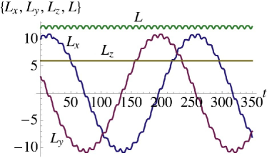
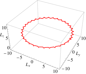
Figure 1: (Color online) $L_{x}(t),L_{y}(t),L_{z}(t)$ and $L(t)=\sqrt{L^{2}_{x}(t)+L^{2}_{y}(t)+L^{2}_{z}(t)}$ (green curve) versus for ${\bf n}(0)=(\sin(\pi/4)\cos(\pi/4),\sin(\pi/4)\sin(\pi/4),\cos(\pi/4))$ and $(L_{x}(0),L_{y}(0),L_{z}(0))=(10,3,6)$.

Another way of expressing the classical equations of motion is in terms of the angular momentum ${\bf L}$ and the unit vector ${\bf n}$,

$$\dot{{\bf n}}=-\frac{1}{I}{\bf L}\times{\bf n}=-{\bm{\omega}}\times{\bf n}.$$ (5)

$$\dot{{\bf L}}=-\alpha({\bf n}\cdot{\bf E})({\bf E}\times{\bf n}).$$ (6)

Figure 1 shows $L_{x}(t),L_{y}(t),L_{z}(t)$, and $L(t)=\sqrt{L^{2}_{x}(t)+L^{2}_{y}(t)+L^{2}_{z}(t)}$ versus time, and Figs. 2 and 3 show $n_{x}(t),n_{y}(t)$, and $n_{z}(t)$ versus time. The dimensionless parameters used in these calculations are $\alpha=1$, $I=20$, and $(E_{x},E_{y},E_{z})=(0,0,1)$, and the initial conditions are taken as, $(L_{x}(0),L_{y}(0),L_{z}(0))=(10,3,6)$, and ${\bf n}(0)=(\sin(\pi/4)\cos(\pi/4),\sin(\pi/4)\sin(\pi/4),\cos(\pi/4))=(1/2,1/2,1/\sqrt{2})$. The dynamics is almost periodic with period of about 250 (dimensionless units).

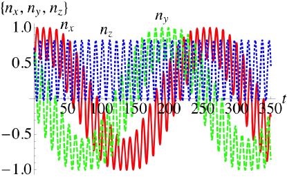
Figure 2: (Color online) $n_{x}(t),n_{y}(t)$, and $n_{z}(t)$ versus time for $n_{x}(0)=n_{y}(0)=1/2$, $n_{z}(0)=1/\sqrt{2}$ (initial conditions for ${\bf L}(t)$ given in Fig. 1 caption).

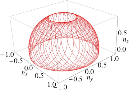
Figure 3: (Color online) Parametric plot of ${\bf n}(t)$ versus time.

III Quantum Treatment

The Hamiltonian for the system is given by $H=\frac{{\hat{L}}^{2}}{2I}-\hat{{\bf d}}\cdot{\bf E}$; taking the induced dipole moment operator to have a component only along the system axis, $\hat{{\bf d}}=(\alpha/2)(\hat{{\bf n}}\cdot{\bf E})\hat{{\bf n}}$, where $\hat{{\bf n}}$ is a vector operator of unit length in the direction of the system axis, we obtain sym_top ,

$$H=\frac{{\hat{L}}^{2}}{2I}-\frac{\alpha}{2}(\hat{{\bf n}}\cdot{\bf E})^{2}.$$ (7)

The Heisenberg equation of motion for $\hat{{\bf n}}$ and $\hat{{\bf L}}$, $\dot{\hat{{\bf n}}}=\frac{i}{\hbar}[H,\hat{{\bf n}}]$ and $\dot{\hat{{\bf n}}}=\frac{i}{\hbar}[H,\hat{{\bf n}}]$, determine the dynamics. For $\dot{\hat{{\bf n}}}$ we find,

$$\dot{\hat{{\bf n}}}=\frac{i}{2\hbar I}[{\hat{L}}^{2},\hat{{\bf n}}]-\frac{i\,\alpha}{2\hbar}[(\hat{{\bf n}}\cdot{\bf E})^{2},\hat{{\bf n}}].$$ (8)

Using the fact that $[\hat{L}_{i},\hat{n}_{j}]=i\hbar\epsilon_{ijk}\hat{n}_{k}$, we obtain, $[{\hat{L}}^{2},\hat{{\bf n}}]=2i\hbar[\hat{{\bf L}}\times\hat{{\bf n}}+i\hbar\,\hat{{\bf n}}]$. Because $[\hat{n}_{i},\hat{n}_{j}]=0$ for all $i$ and $j$, the second term on the RHS of Eq. (8) vanishes, and we find,

$$\dot{\hat{{\bf n}}}=-\frac{1}{I}[\hat{{\bf L}}\times\hat{{\bf n}}+i\hbar\,\hat{{\bf n}}].$$ (9)

The torque on the molecule due to the presence of the external field, $\dot{\hat{{\bf L}}}=\frac{i}{\hbar}[H,\hat{{\bf L}}]$, is given by

$$\dot{\hat{{\bf L}}}=-\alpha(\hat{{\bf n}}\cdot{\bf E})({\bf E}\times\hat{{\bf n}}).$$ (10)

Since the angular momentum is not conserved, the solution of the Heisenberg equations of motion would require a basis set calculation including many angular momentum states; doing so with a stochastic electric field (see Sec. IV) would be very tedious. Therefore, we develop a mean-field approach.

III.1 Mean-Field Dynamics

If the initial angular momentum of the molecule is large compared to $\hbar$, a semiclassical treatment can be a good approximation. Setting $\hbar=0$ in Eq. (9) allows a semiclassical solution for the expectation values $\langle{\hat{{\bf n}}}(t)\rangle$ and $\langle{\hat{{\bf L}}}(t)\rangle$. The semiclassical equations are equivalent to the classical solution presented in Sec. II, and are valid for arbitrary direction of ${\bf E}$. The mean-field theory treatment takes the expectation values of Eqs. (9) and (10), replacing the expectation value of the product $\hat{{\bf L}}\times\hat{{\bf n}}$ by the product of the expectation values Zobay_00 ; Liu_02 ; Tikhonenkov_06 ; Band_07 and taking the limit as $\hbar\to 0$ on the RHS of (9):

$$\langle\dot{\hat{{\bf n}}}\rangle=-\frac{1}{I}\langle{\hat{{\bf L}}}\rangle\times\langle{\hat{{\bf n}}}\rangle,$$ (11)

$$\langle\dot{\hat{{\bf L}}}\rangle=-\alpha(\langle{\hat{{\bf n}}}\rangle\cdot{\bf E})({\bf E}\times\langle{\hat{{\bf n}}}\rangle).$$ (12)

The nonlinear equations of motion, (11) and (12) [which are the same as Eqs. (5) and (6)] must be solved simultaneously.

IV Stochastic Dynamics

We now consider the dynamics in the presence of a stochastic electric field, so the total electric field is taken to be the sum of a deterministic field and a stochastic field, ${\bf E}={\bf E}_{0}+{\bm{\varepsilon}}(t)$, where ${\bm{\varepsilon}}(t)$ is a stochastic process. We solve for the dynamics in two ways. First we treat the stochastic field perturbatively, by dropping the term in the dynamical equations of motion that is quadratic in ${\bm{\varepsilon}}(t)$ and by taking the linear term in ${\bm{\varepsilon}}(t)$ to be Gaussian white noise. Then we treat the full (nonperturbative) dynamics, taking ${\bm{\varepsilon}}(t)$ to be an Ornstein-Uhlenbeck process.

In what follows, we denote the quantum averages of the unit vector along the axis of the molecule and the angular momentum by ${\bf n}(t)\equiv\langle{\hat{{\bf n}}}(t)\rangle$ and ${\bf L}(t)\equiv\langle{\hat{{\bf L}}}(t)\rangle$. The average of these quantities over the stochasticity can be denoted by $\overline{{\bf n}(t)}$ and $\overline{{\bf L}(t)}$ respectively.

IV.1 Perturbation Theory in ${\bm{\varepsilon}}(t)$

In Eq. (12), we substitute ${\bf E}={\bf E}_{0}+{\bm{\varepsilon}}(t)$, and expand, keeping only the linear term in ${\bm{\varepsilon}}(t)$ and dropping the quadratic term. The resulting equation is of the form of a stochastic differential equation. We need only specify the details of the stochastic electric field ${\bm{\varepsilon}}(t)$. We take $\varepsilon_{x}(t)$, $\varepsilon_{y}(t)$ and $\varepsilon_{z}(t)$ to be stochastic processes with zero mean and delta function correlation function $\kappa(t-t^{\prime})$,

$$\overline{\varepsilon_{i}(t)}=0,$$ (13)

$$\overline{\varepsilon_{i}(t)\varepsilon_{j}(t^{\prime})}=\kappa(t-t^{\prime})\,\delta_{ij}=\varepsilon_{0}^{2}\,\delta(t-t^{\prime})\,\delta_{ij},$$ (14)

for $i,j=x,y$ and $z$, i.e., we consider a vector Wiener process. Equations (11) and (12) form a system of differential equations, which can be written in the standard stochastic differential equation form vanKampenBook ,

$$d{\bf n}(t) = -\frac{1}{I}{\bf L}(t)\times{\bf n}(t)\,dt,$$ (15)

$$d{\bf L}(t) = -\alpha\,[({\bf n}(t)\cdot{\bf E}_{0})\,({\bf E}_{0}\times{\bf n}(t))\,dt+({\bf n}(t)\cdot{\bf E}_{0})\,(d{\bm{\varepsilon}}(t)\times{\bf n}(t))+({\bf n}(t)\cdot d{\bm{\varepsilon}}(t))\,({\bf E}_{0}\times{\bf n}(t))],$$ (16)

In the numerical calculations we took ${\bf E}_{0}=(0,0,1)$ (in dimensionless units) and the initial conditions ${\bf n}(0)$ and ${\bf L}(0)$ as in Figs. 1, 2 and 3. Figures 4 and 5 show the vectors ${\bf n}(t)=(n_{x}(t),n_{y}(t),n_{z}(t))$ and ${\bf L}(t)=(L_{x}(t),L_{y}(t),L_{z}(t))$ calculated with the stochastic fields, $\varepsilon_{x}(t)$, $\varepsilon_{y}(t)$ and $\varepsilon_{z}(t)$ taken as Gaussian white noise with a small stochastic field strength (volatility), $\varepsilon_{0}=0.02$. The central curves (in red) give the averages $\overline{{\bf n}(t)}$ and $\overline{{\bf L}(t)}$ in Figs. 4 and 5, and the mean values plus and minus the standard deviations are shown as curves (in blue), with the region between the plus and minus standard deviations shaded (in yellow). Since the initial conditions for the stochastic field is taken to be ${\bm{\varepsilon}}(0)={\bf 0}$, and $\varepsilon_{0}$ is small, the dynamical variables ${\bf n}(t)$ and ${\bf L}(t)$ start off very much like the variables calculated without stochasticity, but by a time of about 250 (dimensionless time units), decoherence is evident. The decoherence becomes significant for times larger than about 400. The variables $n_{x}(t),n_{y}(t)$ and $L_{x}(t),L_{y}(t)$ decay to zero at large times, but $n_{z}(t)$ and $L_{z}(t)$ ‘hang up’ at finite values. It is clear from Eq. (16) that $d\langle L_{z}(t)\rangle/dt=0$, because $d\langle{\bm{\varepsilon}}(t)\rangle/dt=0$ and $({\bf E}_{0}\times{\bf n}(t))_{z}=0$.

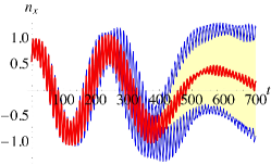
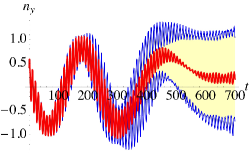
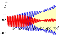
Figure 4: (Color online) Average and standard deviation of $n_{x}(t),n_{y}(t),n_{z}(t)$ versus time obtained for stochastic dynamics using Eqs. (15) and (16) with $\varepsilon_{x}(t)$, $\varepsilon_{y}(t)$ and $\varepsilon_{z}(t)$ fields taken as Gaussian white noise and $\sigma=0.02$.

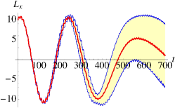
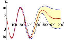
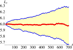
Figure 5: (Color online) Average and standard deviation of the angular momentum vector $(L_{x}(t),L_{y}(t),L_{z}(t))$ versus time obtained for stochastic dynamics using Eqs. (15) and (16) with $\varepsilon_{x}(t)$, $\varepsilon_{y}(t)$ and $\varepsilon_{z}(t)$ fields taken as Gaussian white noise and $\sigma=0.02$.

Figures 6 and 7 are similar to Figs. 4 and 5 and show the average and standard deviation of the vectors ${\bf n}(t)=(n_{x}(t),n_{y}(t),n_{z}(t))$ and ${\bf L}(t)=(L_{x}(t),L_{y}(t),L_{z}(t))$ calculated with a larger value of volatility, $\varepsilon_{0}=0.1$. Now, decoherence sets in at earlier times, becoming significant for times larger than around 150. Again, $\overline{n_{z}(t)}$ and $\overline{L_{z}(t)}$ ‘hang up’ at finite values. Since we expect perturbation theory to begin to break down at larger values of volatility, we now carry out nonperturbative calculations.

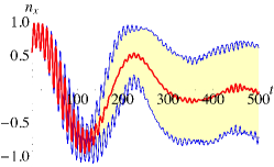
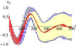
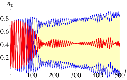
Figure 6: (Color online) Average and standard deviation of $n_{x}(t),n_{y}(t),n_{z}(t)$ versus time obtained for stochastic dynamics using Eqs. (15) and (16) with $\varepsilon_{x}(t)$, $\varepsilon_{y}(t)$ and $\varepsilon_{z}(t)$ fields taken as Gaussian white noise and $\sigma=0.1$.

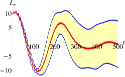
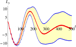
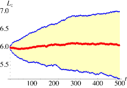
Figure 7: (Color online) Average and standard deviation of the angular momentum vector $(L_{x}(t),L_{y}(t),L_{z}(t))$ versus time obtained for stochastic dynamics using Eqs. (15) and (16) with $\varepsilon_{x}(t)$, $\varepsilon_{y}(t)$ and $\varepsilon_{z}(t)$ fields taken as Gaussian white noise and $\sigma=0.02$.

IV.2 Nonlinear in ${\bm{\varepsilon}}(t)$ Calculation

In order to treat the equations of motion that are nonlinear in the variable ${\bm{\varepsilon}}$, we recast them in the form [recall that we are using the notation ${\bf n}(t)\equiv\langle{\hat{{\bf n}}}(t)\rangle$ and ${\bf L}(t)\equiv\langle{\hat{{\bf L}}}(t)\rangle$],

$$d{\bf n}(t) = -\frac{1}{I}{\bf L}(t)\times{\bf n}(t)\,dt,$$ (17)

$$d{\bf L}(t) = -\alpha\,{\bf n}(t)\cdot[{\bf E}_{0}+{\bm{\varepsilon}}(t)]\,[{\bf E}_{0}+{\bm{\varepsilon}}(t)]\times{\bf n}(t)\,dt,$$ (18)

$$d{\bm{\varepsilon}}(t) = -\vartheta{\bm{\varepsilon}}(t)\,dt+\sigma d{\bf W}(t).$$ (19)

Here $\vartheta$ is the mean reversion rate of the Ornstein-Uhlenbeck process ${\bm{\varepsilon}}$ with long term mean of equal zero, ${\bf W}(t)$ is the standard Wiener process with zero mean and volatility one, and $\sigma$ is the volatility of the Ornstein-Uhlenbeck process. With nonvanishing $\vartheta$, the functional dependence on time of the variance and correlation function of the process ${\bm{\varepsilon}}$ is very different from a Wiener process, but with $\vartheta=0$, the process ${\bm{\varepsilon}}$ is a Wiener process. In the numerical calculations presented here, we take $\vartheta=0$ and initial conditions $\varepsilon_{i}(0)=0$ for $i=1,2,3$.

Figures 8 and 9 show the results of the nonlinear calculation with a value of $\sigma=0.1$. There is a significant difference between the perturbative results shown in Figs. 6 and 7 and the nonperturbative results, even for times as early as $t=25$, and decoherence is already significant for times beyond $t=25$. The most significant difference is that the dynamical variables $n_{z}(t)$ and $L_{z}(t)$ no longer ‘hang up’ at finite values, but decay to zero at large time.

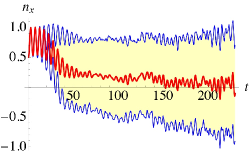
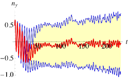
Figure 8: (Color online) Average and standard deviation of $n_{x}(t),n_{y}(t),n_{z}(t)$ versus time obtained for stochastic dynamics using Eqs. (17), (18) and (19), with $\varepsilon_{x}(t)$, $\varepsilon_{y}(t)$ and $\varepsilon_{z}(t)$ fields taken as Gaussian white noise and $\sigma=0.1$.

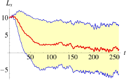
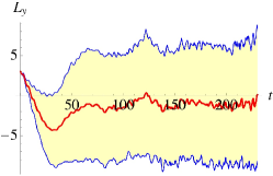
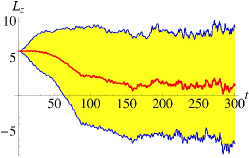
Figure 9: (Color online) Average and standard deviation of the angular momentum vector $(L_{x}(t),L_{y}(t),L_{z}(t))$ versus time obtained for stochastic dynamics using Eqs. (17), (18) and (19), with $\varepsilon_{x}(t)$, $\varepsilon_{y}(t)$ and $\varepsilon_{z}(t)$ fields taken as Gaussian white noise and $\sigma=0.1$.

V Summary and Conclusion

We introduced a model for treating the dynamics of a molecule with an induced dipole moment in the presence of an external electric field. We showed that the classical dynamics is equivalent to the mean-field quantum dynamics of the system. The dynamics is more complicated than the dynamics of a magnetic dipole moment in a magnetic field; modeling the dynamics requires equations of motion for both the angular momentum operator $\hat{{\bf L}}(t)$ and the operator for the unit vector in the direction of the axis of the molecule, $\hat{{\bf n}}(t)$. Then, we considered the dynamics in the presence of an external electric field that is a sum of a deterministic field and a stochastically fluctuating field (noise). For simplicity, we took the fluctuations to be Gaussian white noise. The model makes the external noise assumption vanKampenBook wherein no back-action of the system on the environment is present. Using perturbation theory for the stochastic field, the $z$ component of the average induced electric dipole moment, $\langle{\hat{{\bf n}}}(t)\rangle$, and the $z$ component of the average angular momentum, $\langle{\hat{{\bf L}}}(t)\rangle$, do not decay (decohere) to zero, despite fluctuations in all three components of the electric field, (but the other components of these vectors do decohere). This is in contrast to the decay of the average over fluctuations of a magnetic moment, which does decohere to zero in a stochastic magnetic field with Gaussian white noise in all three components STB_2013 . In contradistinction to the perturbative analysis, i.e., upon including the term nonlinear in the stochastic field in the equations of motion, we find that decoherence occurs in all three components of $\langle\hat{{\bf L}}(t)\rangle$ and $\langle\hat{{\bf n}}(t)\rangle$. Moreover, decoherence of the transverse components of these vectors appears significantly earlier than in the perturbation theory solutions. These predictions, obtained under the external noise assumption, should be able to be readily checked experimentally. These predictions should remain valid also for Gaussian colored noise stochastic processes, as long as the temporal correlation time of the colored noise process, $\tau_{c}$, is short compared with the rotation time of the molecule, $\tau_{r}=I/\langle L\rangle$, and the Stark timescale, $\tau_{S}=\hbar/(Ed)$.

- (1) E. Ishiguro, T. Arai, M. Mizushima and M. Kotani, Proc. Phys. Soc. A65, 178 (1952).
- (2) S. Fleischer, I. S. Averbukh and Y. Prior, Phys. Rev. Lett. 99, 093002 (2007).
- (3) Claudio Scherer, Brazilian J. of Physics 34, 442 (2004).
- (4) P. Szańkowski, M. Trippenbach and Y. B. Band, “Spin Decoherence due to Fluctuating Fields”, arXiv:1211.3032 [cond-mat.mes-hall], Phys. Rev. E (in press).
- (5) Y. B. Band, “The Dynamics of an Electric Dipole Moment in a Stochastic Electric Field”, arXiv: reference.
- (6) N. G. Van Kampen, Stochastic Processes in Physics and Chemistry, (Elsevier, 1997).
- (7) P. E. Kloeden and E. Platen, Numerical Solution of Stochastic Differential Equations, (Springer, 2011).
- (8) For simplicity we take a symmetric top, rather than a spherical top Hamiltonian. If we had taken a symmetric top, , where , is the angular momentum along the body-fixed axis, , and is the unit vector in the direction of the body fixed -axis, the use of angular momentum in the space fixed frame would be required.
- (9) L. D. Landau and E. M. Lifshitz, Quantum Mechanics Non-relativistic Theory, Second Ed., pp. 312-316, and Third Ed., p. 337, Problem 1.
- (10) O. Zobay and B. M. Garraway, Phys. Rev. A61, 033603 (2000).
- (11) J. Liu, L. Fu, B.-Y. Ou, S.-G. Chen, D.-I. Choi, B. Wu, and Q. Niu, Phys. Rev. A66, 023404 (2002).
- (12) I. Tikhonenkov, E. Pazy, Y. B. Band, M. Fleischhauer, and A. Vardi, Phys. Rev. A 73 (2006).
- (13) Y. B. Band, I. Tikhonenkov, E. Pazyy, M. Fleischhauer, and A. Vardi, J. of Modern Optics 54, 697-706 (2007).
- (14) I. Tikhonenkov, E. Pazy, Y. B. Band, M. Fleischhauer, and A. Vardi, Phys. Rev. A 73 (2006).