Partitioned treatment of uncertainty in coupled domain problems: A separated representation approach

Mohammad Hadigol mohammad.hadigol@colorado.edu Alireza Doostan alireza.doostan@colorado.edu Hermann G. Matthies h.matthies@tu-braunschweig.de Rainer Niekamp r.niekamp@tu-bs.de Aerospace Engineering Sciences Department, University of Colorado, Boulder, CO 80309, USA Institute of Scientific Computing, Technische Universität Braunschweig, Braunschweig, Germany
Abstract

This work is concerned with the propagation of uncertainty across coupled domain problems with high-dimensional random inputs. A stochastic model reduction approach based on low-rank separated representations is proposed for the partitioned treatment of the uncertainty space. The construction of the coupled domain solution is achieved though a sequence of approximations with respect to the dimensionality of the random inputs associated with each individual sub-domain and not the combined dimensionality, hence drastically reducing the overall computational cost. The coupling between the sub-domain solutions is done via the classical Finite Element Tearing and Interconnecting (FETI) method, thus providing a well suited framework for parallel computing. Two high-dimensional stochastic problems, a 2D elliptic PDE with random diffusion coefficient and a stochastic linear elasticity problem, have been considered to study the performance and accuracy of the proposed stochastic coupling approach.

keywords:
Uncertainty quantification; Separated representation; Stochastic PDE; Stochastic decoupling; Coupled problem; Domain decomposition; FETI.
journal: Elsevier

1 Introduction

Simulation-based prediction of most physical systems is subject to either lack of knowledge about the governing physical laws or incomplete/limited information about model parameters such as material properties, initial, or boundary conditions. In order to obtain realistic predictions of these systems one, therefore, needs to characterize such uncertainties and quantify their impact on Quantities of interest (QoI). Uncertainty quantification (UQ), an emerging field in computational engineering and science, is concerned with the development of rigorous and efficient solutions to this exercise.

A major class of UQ approaches are probabilistic where uncertain parameters are represented by random variables or processes. Several techniques have been developed to study the propagation of such uncertainties in engineering systems, e.g., see [32, 44, 45, 61, 62, 41] and the references therein. Among these techniques, stochastic spectral methods [32, 31, 65, 62, 41] based on polynomial chaos (PC) expansions [60, 10] have received special attention due to their advantages over traditional UQ techniques such as perturbation-based and Monte Carlo sampling (MCS) methods. In particular, under certain regularity conditions, these schemes converge faster than MCS methods [41] and, unlike perturbation methods, are not restricted to problems with small uncertainty levels [32]. Stochastic spectral methods are based on expanding the solution of interest in PC bases. The coefficients of these expansions are then computed, for instance, via Galerkin projection [32], referred to as stochastic Galerkin (SG), or pseudo-spectral collocation [63, 43], named stochastic collocation (SC).

Although PC-based techniques benefit from elegant mathematical analyses, e.g., formal convergence studies, they may suffer from the so-called curse-of-dimensionality if executed carelessly: the computational cost may grow exponentially as a function of the number of independent random inputs [62, 41, 19], and as a function of the total number of unknowns in the system. This may be a common situation when one is dealing with UQ of engineering problems involving, for instance, coupled domains or separated scales with independent and separate sources of uncertainty. In the past few years, several alternative methods have been proposed to introduce some form of sparsity in an effort to counter the curse-of-dimensionality [43, 63, 57, 8, 7, 48, 46, 18, 40, 25, 28, 49, 6, 67, 19, 36, 14, 1, 29, 35, 20]. The ideas used here are based on sparse grids, element-like partitioning, ANOVA expansions, separated representations, and more general tensor decompositions. Although these techniques have been found efficient in alleviating curse-of-dimensionality, the high computing cost is still a major bottleneck in PC expansion of high-dimensional random solutions.

Of particular interest in the present study is the problem of uncertainty propagation across coupled domain problems where independent, high-dimensional random inputs are present in each sub-domain. In such cases, the solution depends on all random inputs; hence, a direct application of PC expansion may not be feasible or at least not desirable. While integration of PC expansions with standard domain decomposition (DD) techniques may partially reduce the overall computational complexity by partitioning the physical space, e.g., see [33, 15, 56], expansions (or sampling) with respect to the combined set of random inputs is still required. Instead, we propose an approach that additionally enables a partitioned treatment of the stochastic space; that is, the solution is computed through a sequence of approximations with respect to the random inputs associated with each individual sub-domain, and not the combined set of random inputs. To this end, we adopt a stochastic expansion based on the so-called separated representations and demonstrate how it can be obtained in conjunction with a DD approach. As one of the simplest cases of such coupling, we consider a linear problem on two non-overlapping sub-domains with a common interface. Although more elaborate coupling techniques are possible, we restrict ourselves to a finite element tearing and interconnecting (FETI) approach [24] for the sake of simplicity.

Model reduction techniques based on separated representation, a.k.a. canonical decomposition, of high-dimensional stochastic functions have been recently proposed in [47, 17, 18, 48, 49, 36, 35] and proven effective in reducing the issue of curse-of-dimensionality. We here adopt a special form of separated representations for the stochastic computation of coupled domain problems.

Let (Ω,𝒯,𝒫)Ω𝒯𝒫\left(\Omega,\mathcal{T},\mathcal{P}\right) be a complete probability space where ΩΩ\Omega is the sample set and 𝒫𝒫\mathcal{P} is a probability measure on the σlimit-from𝜎\sigma-field 𝒯𝒯\mathcal{T}. Also assume that the input uncertainty has been discretized and approximated by random variables, such that the vector 𝝃=(ξ1,,ξd):Ωd:𝝃subscript𝜉1subscript𝜉𝑑Ωsuperscript𝑑\bm{\xi}=\left(\xi_{1},\cdots,\xi_{d}\right):\Omega\rightarrow\mathbb{R}^{d}, d𝑑d\in\mathbb{N}, represents the set of independent random inputs associated with a PDE defined on a domain 𝒟D𝒟superscript𝐷\mathcal{D}\subset\mathbb{R}^{D}, D{1,2,3}𝐷123D\in\{1,2,3\}, composed of two non-overlapping sub-domains 𝒟1subscript𝒟1\mathcal{D}_{1} and 𝒟2subscript𝒟2\mathcal{D}_{2}. We further assume that the random vector 𝝃=(𝝃1,𝝃2)𝝃subscript𝝃1subscript𝝃2\bm{\xi}=(\bm{\xi}_{1},\bm{\xi}_{2}) is such that 𝝃1:Ωd1:subscript𝝃1Ωsuperscriptsubscript𝑑1\bm{\xi}_{1}:\Omega\rightarrow\mathbb{R}^{d_{1}} and 𝝃2:Ωd2:subscript𝝃2Ωsuperscriptsubscript𝑑2\bm{\xi}_{2}:\Omega\rightarrow\mathbb{R}^{d_{2}} denote random inputs corresponding to 𝒟1subscript𝒟1\mathcal{D}_{1} and 𝒟2subscript𝒟2\mathcal{D}_{2}, respectively. Here, d1,d2subscript𝑑1subscript𝑑2d_{1},d_{2}\in\mathbb{N} are the sizes of 𝝃1subscript𝝃1\bm{\xi}_{1} and 𝝃2subscript𝝃2\bm{\xi}_{2}, respectively, and d=d1+d2𝑑subscript𝑑1subscript𝑑2d=d_{1}+d_{2}. Assuming that u1(𝒙,𝝃):𝒟¯1×Ω:subscript𝑢1𝒙𝝃subscript¯𝒟1Ωu_{1}(\bm{x},\bm{\xi}):\bar{\mathcal{D}}_{1}\times\Omega\rightarrow\mathbb{R} and u2(𝒙,𝝃):𝒟¯2×Ω:subscript𝑢2𝒙𝝃subscript¯𝒟2Ωu_{2}(\bm{x},\bm{\xi}):\bar{\mathcal{D}}_{2}\times\Omega\rightarrow\mathbb{R} are the sub-domain solutions, we consider the separated representation of the form

ui(𝒙,𝝃)=l=1ru0,il(𝒙)ϕ1l(𝝃1)ϕ2l(𝝃2)+𝒪(ϵ),i=1,2.formulae-sequencesubscript𝑢𝑖𝒙𝝃superscriptsubscript𝑙1𝑟superscriptsubscript𝑢0𝑖𝑙𝒙superscriptsubscriptitalic-ϕ1𝑙subscript𝝃1superscriptsubscriptitalic-ϕ2𝑙subscript𝝃2𝒪italic-ϵ𝑖12u_{i}(\bm{x},\bm{\xi})=\sum_{l=1}^{r}{u}_{0,i}^{l}(\bm{x})\phi_{1}^{l}(\bm{\xi}_{1})\phi_{2}^{l}(\bm{\xi}_{2})+\mathcal{O}(\epsilon),\qquad i=1,2. (1)

Here u0,il(𝒙):𝒟¯i:superscriptsubscript𝑢0𝑖𝑙𝒙subscript¯𝒟𝑖u_{0,i}^{l}(\bm{x}):\bar{\mathcal{D}}_{i}\rightarrow\mathbb{R} and ϕil(𝝃i):Ω:superscriptsubscriptitalic-ϕ𝑖𝑙subscript𝝃𝑖Ω\phi_{i}^{l}(\bm{\xi}_{i}):\Omega\rightarrow\mathbb{R}, l=1,,r𝑙1𝑟l=1,\dots,r, are, respectively, deterministic and stochastic functions – or factors – to be determined along with the separation rank r𝑟r. These quantities are not fixed a priori and are computed through an optimization scheme such that a prescribed target accuracy ϵitalic-ϵ\epsilon is reached for a minimum r𝑟r.

Notice that, by definition, finding the expansion (1) is in fact a non-linear problem, even for a linear problem. However, it can be computed through a sequence of alternating linear problems, where {u0,il(𝒙)}l=1rsuperscriptsubscriptsuperscriptsubscript𝑢0𝑖𝑙𝒙𝑙1𝑟\{u_{0,i}^{l}(\bm{x})\}_{l=1}^{r}, i=1,2𝑖12i=1,2, {ϕ1l(𝝃1)}l=1rsuperscriptsubscriptsuperscriptsubscriptitalic-ϕ1𝑙subscript𝝃1𝑙1𝑟\{\phi_{1}^{l}(\bm{\xi}_{1})\}_{l=1}^{r}, or {ϕ2l(𝝃2)}l=1rsuperscriptsubscriptsuperscriptsubscriptitalic-ϕ2𝑙subscript𝝃2𝑙1𝑟\{\phi_{2}^{l}(\bm{\xi}_{2})\}_{l=1}^{r} are solved for one at a time while others are fixed at their recent values. This alternating construction, together with the separated form of (1), enables computing the stochastic functions {ϕ1l(𝝃1)}l=1rsuperscriptsubscriptsuperscriptsubscriptitalic-ϕ1𝑙subscript𝝃1𝑙1𝑟\{\phi_{1}^{l}(\bm{\xi}_{1})\}_{l=1}^{r} and {ϕ2l(𝝃2)}l=1rsuperscriptsubscriptsuperscriptsubscriptitalic-ϕ2𝑙subscript𝝃2𝑙1𝑟\{\phi_{2}^{l}(\bm{\xi}_{2})\}_{l=1}^{r} with computational complexities that depend on d1subscript𝑑1d_{1} and d2subscript𝑑2d_{2} but not d=d1+d2𝑑subscript𝑑1subscript𝑑2d=d_{1}+d_{2}. Additionally, it allows for a natural extension of DD techniques for computing {u0,il(𝒙)}l=1rsuperscriptsubscriptsuperscriptsubscript𝑢0𝑖𝑙𝒙𝑙1𝑟\{u_{0,i}^{l}(\bm{x})\}_{l=1}^{r}. In the present work, we employ the standard FETI approach [24] for the latter purpose. Moreover, for situations where the separation rank r𝑟r is small, (1) provides a reduced order approximation and representation of the coupled solution. We will describe the details of computing (1) in Section 5.

Among the limited earlier effort on separating random inputs for the solution of coupled problems, we particularly mention the recent work of Arnst et al. [3] that is based on the so-called reduced chaos expansions [55]. In particular, in each component, e.g., physics or sub-domain, the solution is expanded in a PC basis that is generated based on random inputs associated with that component. The PC coefficients are then considered to be functions of random inputs corresponding to the other component. This may be seen as a special case of (1). As in (1) we do not prescribe a stochastic basis a priori, our approach is different from that of [3]. The construction of (1) is also different from that of the reduced chaos expansions. More importantly, when the coupled solution admits a low separation rank r𝑟r, the computational complexity and storage requirement of (1) may be significantly smaller than those of the reduced chaos expansion, especially when d𝑑d is large.

Separated representations have also been utilized in the context of multi-scale domain decomposition with high-dimensional local uncertainties [13]. While our coupled domain formulation is similar to that of [13], our particular choice of separated representation (1) and it’s numerical construction, both at the physical and stochastic levels, are considerably different from those in [13].

The remainder of this paper is organized as follows. Section 2 summarizes the problem formulation. There, we start with a general linear stochastic PDE as an abstract problem and present its coupled formulation via FETI. As already remarked, this is one of the simplest problems which has been chosen for the sake of simplicity. The techniques presented here are nonetheless applicable also to non-linear problems and more elaborate coupling schemes, as well as to more than two coupled components. The choice of spatial discretization is given in Section 3 and following that, in Section 4, we review the application of the SG scheme to the original problem as well as its coupled formulation. In Section 5, we present our approach based on separated representations along with an extension of the FETI algorithm to solve the resulting coupled problems at the spatial level. Finally, two numerical examples; a 2D linear diffusion problem on an L-shaped domain with random diffusivity coefficient and a 2D linear elasticity problem describing the deflection of a cantilever beam with random Young’s modulus are considered in Section 6. The accuracy and performance of the proposed coupling approach are demonstrated using these two examples.

2 Problem Formulation

2.1 A linear PDE with random inputs

Let (Ω,𝒯,𝒫)Ω𝒯𝒫\left(\Omega,\mathcal{T},\mathcal{P}\right) be a suitable probability space. We consider computing the solution u(𝒙,𝝃):𝒟¯×Ω:𝑢𝒙𝝃¯𝒟Ωu(\bm{x},\bm{\xi}):\bar{\mathcal{D}}\times\Omega\rightarrow\mathbb{R} satisfying the linear PDE

(𝒙,𝝃)(u(𝒙,𝝃))=f(𝒙)𝒙𝒟,formulae-sequence𝒙𝝃𝑢𝒙𝝃𝑓𝒙𝒙𝒟\displaystyle\mathcal{L}(\bm{x},\bm{\xi})(u(\bm{x},\bm{\xi}))=f(\bm{x})\ \ \ \ \ \bm{x}\in\mathcal{D}, (2)
(𝒙,𝝃)(u(𝒙,𝝃))=g(𝒙)𝒙𝒟,formulae-sequence𝒙𝝃𝑢𝒙𝝃𝑔𝒙𝒙𝒟\displaystyle\mathcal{B}(\bm{x},\bm{\xi})(u(\bm{x},\bm{\xi}))=g(\bm{x})\ \ \ \ \bm{x}\in\partial\mathcal{D},

𝒫limit-from𝒫\mathcal{P}- almost surely in ΩΩ\Omega. Here, 𝒟D𝒟superscript𝐷\mathcal{D}\subset\mathbb{R}^{D}, D𝐷D=1,2,3, is the spatial extent of the problem with boundary 𝒟𝒟\partial\mathcal{D} as displayed in Fig. 1, \mathcal{L} is a linear differential operator, and \mathcal{B} is a boundary operator taking possibly various forms on different boundary segments. We assume (2) is the variational equation associated with a minimization problem. Additionally, as mentioned before, the uncertainty in (2) is assumed to have been approximated in such a way it may be represented by the random vector 𝝃=(ξ1,,ξd):Ωd,d:𝝃subscript𝜉1subscript𝜉𝑑formulae-sequenceΩsuperscript𝑑𝑑\bm{\xi}=\left(\xi_{1},\cdots,\xi_{d}\right):\Omega\rightarrow\mathbb{R}^{d},d\in\mathbb{N}, consisting of independent identically distributed (i.i.d.) random variables ξksubscript𝜉𝑘\xi_{k} with probability density function ρ(ξk):+:𝜌subscript𝜉𝑘subscript\rho(\xi_{k}):\mathbb{R}\rightarrow\mathbb{R}_{+}. Without loss of generality, the functions f(𝒙)𝑓𝒙f(\bm{x}) and g(𝒙)𝑔𝒙g(\bm{x}) in (2) are considered to be deterministic. We hereafter refer to (2) as the original problem.

Refer to caption

𝒟1subscript𝒟1\mathcal{D}_{1}𝒟2subscript𝒟2\mathcal{D}_{2}𝒟1subscript𝒟1\partial\mathcal{D}_{1}𝒟2subscript𝒟2\partial\mathcal{D}_{2}ΓIsubscriptΓ𝐼\Gamma_{I}

Figure 1: Geometry of the original problem and partitioning of 𝒟𝒟\mathcal{D} into two non-overlapping sub-domains 𝒟1subscript𝒟1\mathcal{D}_{1} and 𝒟2subscript𝒟2\mathcal{D}_{2}. 𝒟=𝒟1𝒟2𝒟subscript𝒟1subscript𝒟2\mathcal{D}=\mathcal{D}_{1}\cup\mathcal{D}_{2}, 𝒟1𝒟2=subscript𝒟1subscript𝒟2\mathcal{D}_{1}\cap\mathcal{D}_{2}=\emptyset, and 𝒟1𝒟2=ΓIsubscript𝒟1subscript𝒟2subscriptΓ𝐼\partial\mathcal{D}_{1}\cap\partial\mathcal{D}_{2}=\Gamma_{I}.

We assume that 𝒟𝒟\mathcal{D} is composed of two non-overlapping sub-domains 𝒟1subscript𝒟1\mathcal{D}_{1} and 𝒟2subscript𝒟2\mathcal{D}_{2} (𝒟=𝒟1𝒟2𝒟subscript𝒟1subscript𝒟2\mathcal{D}=\mathcal{D}_{1}\cup\mathcal{D}_{2} and 𝒟1𝒟2=subscript𝒟1subscript𝒟2\mathcal{D}_{1}\cap\mathcal{D}_{2}=\emptyset) sharing an interface boundary ΓI=𝒟1𝒟2subscriptΓ𝐼subscript𝒟1subscript𝒟2\Gamma_{I}=\partial\mathcal{D}_{1}\cap\partial\mathcal{D}_{2} as shown in Fig. 1. We further assume that the random inputs representing the uncertainty in 𝒟1subscript𝒟1\mathcal{D}_{1} and 𝒟2subscript𝒟2\mathcal{D}_{2} are independent and denoted by 𝝃1=(ξ1,1,,ξ1,d1):Ωd1,d1:subscript𝝃1subscript𝜉11subscript𝜉1subscript𝑑1formulae-sequenceΩsuperscriptsubscript𝑑1subscript𝑑1\bm{\xi}_{1}=\left(\xi_{1,1},\cdots,\xi_{1,d_{1}}\right):{\color[rgb]{0,0,0}\Omega\rightarrow\mathbb{R}^{d_{1}}},d_{1}\in\mathbb{N} and 𝝃2=(ξ2,1,,ξ2,d2):Ωd2,d2:subscript𝝃2subscript𝜉21subscript𝜉2subscript𝑑2formulae-sequenceΩsuperscriptsubscript𝑑2subscript𝑑2\bm{\xi}_{2}=\left(\xi_{2,1},\cdots,\xi_{2,d_{2}}\right):{\color[rgb]{0,0,0}\Omega\rightarrow\mathbb{R}^{d_{2}}},d_{2}\in\mathbb{N}, respectively. This, therefore, provides a natural partitioning of 𝝃𝝃\bm{\xi} into 𝝃=(𝝃1,𝝃2)𝝃subscript𝝃1subscript𝝃2\bm{\xi}=(\bm{\xi}_{1},\bm{\xi}_{2}).

We note that while we consider the case of two coupled sub-domains, the extension of the subsequent algorithms to the case of multiple coupled sub-domains is straight-forward.

2.2 The coupled formulation of original problem

We next reformulate the original problem (2) in terms of the coupled stochastic PDEs,

(𝒙,𝝃1)(u1(𝒙,𝝃))=f(𝒙)𝒙𝒟1,formulae-sequence𝒙subscript𝝃1subscript𝑢1𝒙𝝃𝑓𝒙𝒙subscript𝒟1\displaystyle\mathcal{L}(\bm{x},\bm{\xi}_{1})(u_{1}(\bm{x},\bm{\xi}))=f(\bm{x})\ \ \ \ \ \ \bm{x}\in\mathcal{D}_{1}, (3)
(𝒙,𝝃2)(u2(𝒙,𝝃))=f(𝒙)𝒙𝒟2,formulae-sequence𝒙subscript𝝃2subscript𝑢2𝒙𝝃𝑓𝒙𝒙subscript𝒟2\displaystyle\mathcal{L}(\bm{x},\bm{\xi}_{2})(u_{2}(\bm{x},\bm{\xi}))=f(\bm{x})\ \ \ \ \ \ \bm{x}\in\mathcal{D}_{2},
(𝒙,𝝃1)(u1(𝒙,𝝃))=g(𝒙)𝒙𝒟1,formulae-sequence𝒙subscript𝝃1subscript𝑢1𝒙𝝃𝑔𝒙𝒙subscript𝒟1\displaystyle\mathcal{B}(\bm{x},\bm{\xi}_{1})(u_{1}(\bm{x},\bm{\xi}))=g(\bm{x})\ \ \ \ \ \ \bm{x}\in\partial\mathcal{D}_{1},
(𝒙,𝝃2)(u2(𝒙,𝝃))=g(𝒙)𝒙𝒟2,formulae-sequence𝒙subscript𝝃2subscript𝑢2𝒙𝝃𝑔𝒙𝒙subscript𝒟2\displaystyle\mathcal{B}(\bm{x},\bm{\xi}_{2})(u_{2}(\bm{x},\bm{\xi}))=g(\bm{x})\ \ \ \ \ \ \bm{x}\in\partial\mathcal{D}_{2},
u1(𝒙,𝝃)=u2(𝒙,𝝃)𝒙ΓI,formulae-sequencesubscript𝑢1𝒙𝝃subscript𝑢2𝒙𝝃𝒙subscriptΓ𝐼\displaystyle u_{1}(\bm{x},\bm{\xi})=u_{2}(\bm{x},\bm{\xi})\quad\quad\ \ \ \ \ \ \ \ \ \bm{x}\in\Gamma_{I},

which we henceforth refer to as the coupled problem. Here, u1(𝒙,𝝃):𝒟¯1×Ω:subscript𝑢1𝒙𝝃subscript¯𝒟1Ωu_{1}(\bm{x},\bm{\xi}):\bar{\mathcal{D}}_{1}\times\Omega\rightarrow\mathbb{R} and u2(𝒙,𝝃):𝒟¯2×Ω:subscript𝑢2𝒙𝝃subscript¯𝒟2Ωu_{2}(\bm{x},\bm{\xi}):\bar{\mathcal{D}}_{2}\times\Omega\rightarrow\mathbb{R} are the solutions to (3). The last equation in (3) enforces the continuity of the solution on the interface ΓIsubscriptΓ𝐼\Gamma_{I}. Again, for the sake of simplicity, we tacitly assume that the last equation in (3) is sufficient to enforce that the two partial solutions u1(𝒙,𝝃)subscript𝑢1𝒙𝝃u_{1}(\bm{x},\bm{\xi}) and u2(𝒙,𝝃)subscript𝑢2𝒙𝝃u_{2}(\bm{x},\bm{\xi}) of (3) agree with the restriction of the solution u(𝒙,𝝃)𝑢𝒙𝝃u(\bm{x},\bm{\xi}) of (2) to the respective sub-domains. Our goal is then to find the sub-domain solutions u1(𝒙,𝝃)subscript𝑢1𝒙𝝃u_{1}(\bm{x},\bm{\xi}) and u2(𝒙,𝝃)subscript𝑢2𝒙𝝃u_{2}(\bm{x},\bm{\xi}) assuming independent solvers for each sub-domain.

In the following section, we will discuss the spatial discretization of the original and coupled problems.

3 Spatial Discretization

3.1 Original problem

Let 𝒳𝒳\mathcal{X} be a suitable Hilbert space for the spatial discretization of the solution to the variational formulation of (2). For example, if \mathcal{L} in (2) is a linear elliptic differential operator of second order and \mathcal{B} corresponds to a homogeneous Dirichlet boundary condition, then 𝒳:=H01(𝒟)={vH1(𝒟):v=0\mathcal{X}:=H^{1}_{0}(\mathcal{D})=\{v\in H^{1}(\mathcal{D}):v=0 on 𝒟}\partial\mathcal{D}\}. Also let 𝒲:=L2(Ω)={v:Ω:𝔼[v2]=Ωv2𝒫(dv)<}assign𝒲subscript𝐿2Ωconditional-set𝑣:Ω𝔼delimited-[]superscript𝑣2subscriptΩsuperscript𝑣2𝒫d𝑣\mathcal{W}:=L_{2}(\Omega)=\{v:\Omega\rightarrow\mathbb{R}:\mathbb{E}[v^{2}]=\int_{\Omega}v^{2}\mathcal{P}(\mathrm{d}{v})<\infty\} be the space of all square integrable random variables defined on (Ω,𝒯,𝒫)Ω𝒯𝒫\left(\Omega,\mathcal{T},\mathcal{P}\right). Here, 𝔼[]𝔼delimited-[]\mathbb{E}[\cdot] denotes the mathematical expectation operator. The solution u(𝒙,𝝃)𝑢𝒙𝝃u(\bm{x},\bm{\xi}) to (2) then lives in the tensor-product space 𝒳𝒲tensor-product𝒳𝒲\mathcal{X}\otimes\mathcal{W} [44].

A finite dimensional subspace 𝒳h𝒳subscript𝒳𝒳\mathcal{X}_{h}\subset\mathcal{X} may be constructed by considering a finite element (FE) discretization consisting of piecewise linear, continuous functions {Nm(𝒙)}m=1Msuperscriptsubscriptsubscript𝑁𝑚𝒙𝑚1𝑀\{N_{m}(\bm{x})\}_{m=1}^{M} on a triangulation of 𝒟𝒟\mathcal{D} with a uniform mesh size hh. The approximate solution uhsubscript𝑢u_{h} to the original problem (2) can then be written in the form

uh(𝒙,𝝃)=m=1Mum(𝝃)Nm(𝒙).subscript𝑢𝒙𝝃superscriptsubscript𝑚1𝑀subscript𝑢𝑚𝝃subscript𝑁𝑚𝒙u_{h}(\bm{x},\bm{\xi})=\sum_{m=1}^{M}u_{m}(\bm{\xi})N_{m}(\bm{x}). (4)

We denote by 𝒖(𝝃)=[u1(𝝃),,uM(𝝃)]TM𝒲𝒖𝝃superscriptsubscript𝑢1𝝃subscript𝑢𝑀𝝃𝑇tensor-productsuperscript𝑀𝒲\bm{u}(\bm{\xi})=[u_{1}(\bm{\xi}),\cdots,u_{M}(\bm{\xi})]^{T}\in\mathbb{R}^{M}\otimes\mathcal{W} the random vector of expansion coefficients in (4) given by the Galerkin projection of (2) onto 𝒳hsubscript𝒳\mathcal{X}_{h}. Specifically,

𝑲(𝝃)𝒖(𝝃)=𝒇,𝑲𝝃𝒖𝝃𝒇\displaystyle\bm{K}(\bm{\xi})\bm{u}(\bm{\xi})=\bm{f}, (5)

where 𝑲(𝝃):ΩM×M:𝑲𝝃Ωsuperscript𝑀𝑀\bm{K}(\bm{\xi}):\Omega\rightarrow\mathbb{R}^{M\times M} is the random stiffness matrix – assumed to be symmetric, positive definite 𝒫limit-from𝒫\mathcal{P}- almost surely in ΩΩ\Omega – and 𝒇M𝒇superscript𝑀\bm{f}\in\mathbb{R}^{M} is the deterministic force vector.

We next give a brief discussion on a number of domain decomposition techniques as well as our approach for spatial discretization of the coupled problem (3).

3.2 Coupled problem

Domain decomposition (DD) methods have been found efficient and powerful means for solving large-scale PDEs with parallel computing [11, 51, 54, 2, 34]. The main idea of DD is to decompose 𝒟𝒟\mathcal{D} into a number of smaller overlapping or non-overlapping sub-domains, and to compute the solution on each sub-domain to obtain the solution over the original domain [66, 9]. This is a special case of a partitioned solution approach.

In the present study we assume that the partitioning of 𝒟𝒟\mathcal{D} results in non-overlapping sub-domains. Non-overlapping DD methods, also known as iterative sub-structuring methods [2, 34], have some advantages over overlapping DD schemes, e.g., in being more efficient in handling elliptic problems with large jumps in the coefficients [66]. These methods can be classified based on the treatment of the interface solution compatibility. Primal methods, such as balancing domain decomposition (BDD) [38] and balancing domain decomposition by constraints (BDDC) [16], enforce the continuity constraint on the sub-domains interfaces via computing a unique unknown interface solution. Alternatively, in dual methods, e.g., the FETI algorithm [24], this is done by iterating on intermediary unknown variables, i.e., Lagrange multipliers. There are also hybrid methods such as dual–primal finite element tearing and interconnecting (FETI-DP) [22], that are based on the combination of these two approaches. In the present work, as mentioned in Section 1, we use the classical FETI algorithm towards computing the coupled solution to (3). However, we note that our approach may also be integrated with other non-overlapping DD techniques, specially the FETI-DP. The FETI method is based on finding the stationary or saddle point of an energy functional associated with the sub-domain solutions, which we will discuss next.

Let 𝒖1(𝝃)M1𝒲subscript𝒖1𝝃tensor-productsuperscriptsubscript𝑀1𝒲\bm{u}_{1}(\bm{\xi})\in\mathbb{R}^{M_{1}}\otimes\mathcal{W} and 𝒖2(𝝃)M2𝒲subscript𝒖2𝝃tensor-productsuperscriptsubscript𝑀2𝒲\bm{u}_{2}(\bm{\xi})\in\mathbb{R}^{M_{2}}\otimes\mathcal{W} be the vector of nodal values corresponding to the FE discretization of u1subscript𝑢1u_{1} and u2subscript𝑢2u_{2} in (3), respectively. For simplicity, we assume that the triangulations of 𝒟1subscript𝒟1\mathcal{D}_{1} and 𝒟2subscript𝒟2\mathcal{D}_{2} result in matching nodes at the interface ΓIsubscriptΓ𝐼\Gamma_{I} with MIsubscript𝑀𝐼M_{I} degrees of freedom. Let also 𝝀(𝝃)=[λ1(𝝃),,λMI(𝝃)]TMI𝒲𝝀𝝃superscriptsubscript𝜆1𝝃subscript𝜆subscript𝑀𝐼𝝃𝑇tensor-productsuperscriptsubscript𝑀𝐼𝒲\bm{\lambda}(\bm{\xi})=[\lambda_{1}(\bm{\xi}),\cdots,\lambda_{M_{I}}(\bm{\xi})]^{T}\in\mathbb{R}^{M_{I}}\otimes\mathcal{W} be the random vector of Lagrange multipliers to enforce the solution continuity at ΓIsubscriptΓ𝐼\Gamma_{I}. Then the triple (𝒖1,𝒖2,𝝀)subscript𝒖1subscript𝒖2𝝀(\bm{u}_{1},\bm{u}_{2},\bm{\lambda}) is the stationary point of the energy functional

π(𝒖1,𝒖2,𝝀)=𝜋subscript𝒖1subscript𝒖2𝝀absent\displaystyle\pi(\bm{u}_{1},\bm{u}_{2},\bm{\lambda})= (6)
𝔼[12𝒖1T𝑲1𝒖1𝒖1T𝒇1]+𝔼[12𝒖2T𝑲2𝒖2𝒖2T𝒇2]+𝔼[𝝀T(𝑪2T𝒖2𝑪1T𝒖1)],𝔼delimited-[]12superscriptsubscript𝒖1𝑇subscript𝑲1subscript𝒖1superscriptsubscript𝒖1𝑇subscript𝒇1𝔼delimited-[]12superscriptsubscript𝒖2𝑇subscript𝑲2subscript𝒖2superscriptsubscript𝒖2𝑇subscript𝒇2𝔼delimited-[]superscript𝝀𝑇superscriptsubscript𝑪2𝑇subscript𝒖2superscriptsubscript𝑪1𝑇subscript𝒖1\displaystyle\mathbb{E}\left[\frac{1}{2}\bm{u}_{1}^{T}\bm{K}_{1}\bm{u}_{1}-\bm{u}_{1}^{T}\bm{f}_{1}\right]+\mathbb{E}\left[\frac{1}{2}\bm{u}_{2}^{T}\bm{K}_{2}\bm{u}_{2}-\bm{u}_{2}^{T}\bm{f}_{2}\right]+\mathbb{E}\left[\bm{\lambda}^{T}\left(\bm{C}_{2}^{T}\bm{u}_{2}-\bm{C}_{1}^{T}\bm{u}_{1}\right)\right],

where, for i=1,2𝑖12i=1,2, 𝑪iMi×MIsubscript𝑪𝑖superscriptsubscript𝑀𝑖subscript𝑀𝐼\bm{C}_{i}\in\mathbb{R}^{M_{i}\times M_{I}} are matrices that extract the interface nodal solutions from 𝒖isubscript𝒖𝑖\bm{u}_{i} and 𝑲i(𝝃i):ΩMi×Mi:subscript𝑲𝑖subscript𝝃𝑖Ωsuperscriptsubscript𝑀𝑖subscript𝑀𝑖\bm{K}_{i}(\bm{\xi}_{i}):\Omega\rightarrow\mathbb{R}^{M_{i}\times M_{i}} and 𝒇iMisubscript𝒇𝑖superscriptsubscript𝑀𝑖\bm{f}_{i}\in\mathbb{R}^{M_{i}}, are, respectively, the random stiffness matrices and deterministic force vectors associated with the FE discretization of (3) on 𝒟isubscript𝒟𝑖\mathcal{D}_{i}.

Assumption 1.

In the present study, we assume that 𝐊1(𝛏1)subscript𝐊1subscript𝛏1\bm{K}_{1}(\bm{\xi}_{1}) is symmetric positive definite, while 𝐊2(𝛏2)subscript𝐊2subscript𝛏2\bm{K}_{2}(\bm{\xi}_{2}) is symmetric positive semi-definite (which includes definite) 𝒫limit-from𝒫\mathcal{P}-almost surely in ΩΩ\Omega.

Given Assumption 1, the coupled solution (𝒖1,𝒖2,𝝀)subscript𝒖1subscript𝒖2𝝀(\bm{u}_{1},\bm{u}_{2},\bm{\lambda}) can be obtained by solving the following saddle point problem, established by the first-order optimality condition corresponding to the stationary point of π𝜋\pi in (6),

[𝑲1(𝝃1)𝟎𝑪1𝟎𝑲2(𝝃2)𝑪2𝑪1T𝑪2T𝟎]{𝒖1(𝝃)𝒖2(𝝃)𝝀(𝝃)}={𝒇1𝒇2𝟎},or𝑲c(𝝃)𝒖c(𝝃)=𝒇c.formulae-sequencedelimited-[]subscript𝑲1subscript𝝃10subscript𝑪10subscript𝑲2subscript𝝃2subscript𝑪2superscriptsubscript𝑪1𝑇superscriptsubscript𝑪2𝑇0subscript𝒖1𝝃subscript𝒖2𝝃𝝀𝝃subscript𝒇1subscript𝒇20orsubscript𝑲𝑐𝝃subscript𝒖𝑐𝝃subscript𝒇𝑐\displaystyle\left[\begin{array}[]{ccc}\bm{K}_{1}(\bm{\xi}_{1})&\bm{0}&\bm{C}_{1}\\ \bm{0}&\bm{K}_{2}(\bm{\xi}_{2})&-\bm{C}_{2}\\ {\bm{C}_{1}}^{T}&-{\bm{C}_{2}}^{T}&\bm{0}\end{array}\right]\left\{\begin{array}[]{c}\bm{u}_{1}(\bm{\xi})\\ \bm{u}_{2}(\bm{\xi})\\ \bm{\lambda}(\bm{\xi})\end{array}\right\}=\left\{\begin{array}[]{c}\bm{f}_{1}\\ \bm{f}_{2}\\ \bm{0}\end{array}\right\},\quad\mathrm{or}\quad\bm{K}_{c}(\bm{\xi})\bm{u}_{c}(\bm{\xi})=\bm{f}_{c}. (16)

The deterministic version of (16), i.e., corresponding to fixed realizations of 𝝃1subscript𝝃1\bm{\xi}_{1} and 𝝃2subscript𝝃2\bm{\xi}_{2}, may be solved efficiently using the FETI method, described in Section 5.2. This is done by eliminating the primal variables 𝒖1subscript𝒖1\bm{u}_{1} and 𝒖2subscript𝒖2\bm{u}_{2} form (16) and then solving the resulting system of equations for the dual variable 𝝀𝝀\bm{\lambda} using a projected conjugate gradient solver [24].

We next present a stochastic discretization of (5) and (16) using the standard PC expansions. Following that, in Section 5, we introduce the proposed stochastic discretization which allows us to solve (16) iteratively through approximations in terms of 𝝃1subscript𝝃1\bm{\xi}_{1} or 𝝃2subscript𝝃2\bm{\xi}_{2}.

4 Stochastic Discretization via Polynomial Chaos

Similar to spatial discretization, the first step in performing a stochastic discretization is to select an expansion basis. Several choices have been suggested for this purpose, e.g., polynomial chaos (PC) [32, 64], piecewise polynomial [4], and a multi-wavelet [42] basis. In practice, the choice of expansion basis depends on the probability distribution of 𝝃𝝃\bm{\xi} and the regularity of the solution with respect to 𝝃𝝃\bm{\xi}. In the present study, for the sake of simplicity, we use the PC for the stochastic discretization.

Let ψik(ξk)subscript𝜓subscript𝑖𝑘subscript𝜉𝑘\psi_{{i}_{k}}(\xi_{k}), k=1,,d𝑘1𝑑k=1,\dots,d, be a polynomial of degree ik0:={0}subscript𝑖𝑘subscript0assign0{i}_{k}\in\mathbb{N}_{0}:=\mathbb{N}\cup\{0\} orthogonal with respect to the measure ρ(ξk)𝜌subscript𝜉𝑘\rho(\xi_{k}), i.e.,

𝔼[ψikψjk]=ψik(ξk)ψjk(ξk)ρ(ξk)dξk=δikjk𝔼[ψik2],𝔼delimited-[]subscript𝜓subscript𝑖𝑘subscript𝜓subscript𝑗𝑘subscript𝜓subscript𝑖𝑘subscript𝜉𝑘subscript𝜓subscript𝑗𝑘subscript𝜉𝑘𝜌subscript𝜉𝑘differential-dsubscript𝜉𝑘subscript𝛿subscript𝑖𝑘subscript𝑗𝑘𝔼delimited-[]superscriptsubscript𝜓subscript𝑖𝑘2\mathbb{E}[\psi_{i_{k}}\psi_{j_{k}}]=\int\psi_{i_{k}}(\xi_{k})\psi_{j_{k}}(\xi_{k})\rho(\xi_{k})\mathrm{d}\xi_{k}=\delta_{i_{k}j_{k}}\mathbb{E}[\psi_{i_{k}}^{2}], (17)

where δikjksubscript𝛿subscript𝑖𝑘subscript𝑗𝑘\delta_{i_{k}j_{k}} is the Kronecker delta. The polynomial chaos of maximum (total) degree p0𝑝subscript0p\in\mathbb{N}_{0} is then obtained by the tensorization of ψik(ξk)subscript𝜓subscript𝑖𝑘subscript𝜉𝑘\psi_{{i}_{k}}(\xi_{k}) corresponding to different directions k𝑘k,

ψ𝒊(𝝃)=k=1dψik(ξk),𝒊d,p,formulae-sequencesubscript𝜓𝒊𝝃superscriptsubscriptproduct𝑘1𝑑subscript𝜓subscript𝑖𝑘subscript𝜉𝑘𝒊subscript𝑑𝑝\psi_{\bm{i}}(\bm{\xi})=\prod_{k=1}^{d}\psi_{{i}_{k}}(\xi_{k}),\ \ \ \ \bm{i}\in\mathscr{I}_{d,p}, (18)

where 𝒊=(i1,,id)d,p𝒊subscript𝑖1subscript𝑖𝑑subscript𝑑𝑝{\bm{i}}=(i_{1},\cdots,i_{d})\in\mathscr{I}_{d,p} and the set of multi-indeces d,psubscript𝑑𝑝\mathscr{I}_{d,p} is defined by

d,p={𝒊=(i1,,id)0d:𝒊1p}.subscript𝑑𝑝conditional-set𝒊subscript𝑖1subscript𝑖𝑑superscriptsubscript0𝑑subscriptnorm𝒊1𝑝\mathscr{I}_{d,p}=\{\bm{i}=(i_{1},\cdots,i_{d})\in\mathbb{N}_{0}^{d}:\|\bm{i}\|_{1}\leqslant p\}. (19)

The cardinality of d,psubscript𝑑𝑝\mathscr{I}_{d,p}, hence the number of PC basis functions of total order not larger than p𝑝p in dimension d𝑑d, is given by

P=|d,p|=(p+d)!p!d!.𝑃subscript𝑑𝑝𝑝𝑑𝑝𝑑P=|\mathscr{I}_{d,p}|=\frac{(p+d)!}{p!d!}. (20)

Although the total order truncation is used here for simplicity, this gives only very coarse control of the size of the basis. It is therefore advisable to use some finer method to control the size of the basis, preferably in an adaptive or at least heuristic fashion, see, e.g., [8, 7].

Following the orthogonality of the polynomials ψik(ξk)subscript𝜓subscript𝑖𝑘subscript𝜉𝑘\psi_{{i}_{k}}(\xi_{k}) and given that the ξksubscript𝜉𝑘\xi_{k} are independent, the PC basis functions ψ𝒊(𝝃)subscript𝜓𝒊𝝃\psi_{\bm{i}}(\bm{\xi}) are also orthogonal, i.e., 𝔼[ψ𝒊ψ𝒋]=δ𝒊,𝒋𝔼[ψ𝒊2]𝔼delimited-[]subscript𝜓𝒊subscript𝜓𝒋subscript𝛿𝒊𝒋𝔼delimited-[]superscriptsubscript𝜓𝒊2\mathbb{E}[\psi_{\bm{i}}\psi_{\bm{j}}]=\delta_{\bm{i},\bm{j}}\mathbb{E}[\psi_{\bm{i}}^{2}].

We define the finite dimensional space

𝒲p=span{ψ𝒊(𝝃):𝒊d,p}𝒲,subscript𝒲𝑝spanconditional-setsubscript𝜓𝒊𝝃𝒊subscript𝑑𝑝𝒲\mathcal{W}_{p}=\mathrm{span}\{\psi_{\bm{i}}(\bm{\xi}):\bm{i}\in\mathscr{I}_{d,p}\}\subset\mathcal{W},

within which we seek an approximation to a finite-variance, stochastic function u(𝝃)𝒲𝑢𝝃𝒲u(\bm{\xi})\in\mathcal{W} by

up(𝝃)=𝒊d,pu𝒊ψ𝒊(𝝃).subscript𝑢𝑝𝝃subscript𝒊subscript𝑑𝑝subscript𝑢𝒊subscript𝜓𝒊𝝃u_{p}(\bm{\xi})=\sum_{\bm{i}\in\mathscr{I}_{d,p}}u_{\bm{i}}\psi_{\bm{i}}(\bm{\xi}). (21)

The PC coefficients u𝒊subscript𝑢𝒊u_{\bm{i}} are given by

u𝒊=𝔼[uψ𝒊]𝔼[ψ𝒊2]subscript𝑢𝒊𝔼delimited-[]𝑢subscript𝜓𝒊𝔼delimited-[]superscriptsubscript𝜓𝒊2u_{\bm{i}}=\frac{\mathbb{E}[u\psi_{\bm{i}}]}{\mathbb{E}[\psi_{\bm{i}}^{2}]} (22)

and the series in (21) converges in the mean-square sense as p𝑝p\to\infty.

For the solutions to the original and coupled problems (5) and (16), respectively, the direct projection (22) may not be applied to compute the PC coefficients, unless (22) is computed using random sampling or quadrature integration. Alternatively, as proposed in [32], the PC coefficients may be computed via Galerkin projection that we briefly describe next.

4.1 Galerkin projection

Let 𝒖p(𝝃)=𝒊d,p𝒖𝒊ψ𝒊(𝝃)subscript𝒖𝑝𝝃subscript𝒊subscript𝑑𝑝subscript𝒖𝒊subscript𝜓𝒊𝝃\bm{u}_{p}(\bm{\xi})=\sum_{\bm{i}\in\mathscr{I}_{d,p}}\bm{u}_{\bm{i}}\psi_{\bm{i}}(\bm{\xi}) be the PC approximation to the exact solution 𝒖(𝝃)𝒖𝝃\bm{u}(\bm{\xi}) to (5). The coefficients 𝒖isubscript𝒖𝑖\bm{u}_{i} can be computed from the Galerkin projection

𝔼[𝒗T(𝑲𝒖p𝒇)]=0,𝒗M𝒲p,formulae-sequence𝔼delimited-[]superscript𝒗𝑇𝑲subscript𝒖𝑝𝒇0for-all𝒗tensor-productsuperscript𝑀subscript𝒲𝑝\displaystyle\mathbb{E}[\bm{v}^{T}(\bm{K}{\bm{u}_{p}}-\bm{f})]=0,\ \ \ \ \ \ \ \forall\bm{v}\in\mathbb{R}^{M}\otimes\mathcal{W}_{p},

which can be equivalently written in the form of the coupled system of equations

𝒊d,p𝔼[ψ𝒊ψ𝒋𝑲]𝒖𝒊=𝔼[ψ𝒋𝒇],𝒋d,p.formulae-sequencesubscript𝒊subscript𝑑𝑝𝔼delimited-[]subscript𝜓𝒊subscript𝜓𝒋𝑲subscript𝒖𝒊𝔼delimited-[]subscript𝜓𝒋𝒇for-all𝒋subscript𝑑𝑝\sum_{\bm{i}\in\mathscr{I}_{d,p}}\mathbb{E}[\psi_{\bm{i}}\psi_{\bm{j}}\bm{K}]\bm{u}_{\bm{i}}=\mathbb{E}[\psi_{\bm{j}}\bm{f}],\ \ \ \ \ \ \ \forall\bm{j}\in\mathscr{I}_{d,p}. (23)

Following the same procedure, the Galerkin solution of the coupled problem (16) is computed from

𝒊d,p𝔼[ψ𝒊ψ𝒋𝑲c]𝒖c,𝒊=𝔼[ψ𝒋𝒇c],𝒋d,p,formulae-sequencesubscript𝒊subscript𝑑𝑝𝔼delimited-[]subscript𝜓𝒊subscript𝜓𝒋subscript𝑲𝑐subscript𝒖𝑐𝒊𝔼delimited-[]subscript𝜓𝒋subscript𝒇𝑐for-all𝒋subscript𝑑𝑝\sum_{\bm{i}\in\mathscr{I}_{d,p}}\mathbb{E}[\psi_{\bm{i}}\psi_{\bm{j}}\bm{K}_{c}]{\bm{u}}_{c,\bm{i}}=\mathbb{E}[\psi_{\bm{j}}\bm{f}_{c}],\ \ \ \ \ \ \ \forall\bm{j}\in\mathscr{I}_{d,p}, (24)

where 𝑲csubscript𝑲𝑐\bm{K}_{c} and 𝒇csubscript𝒇𝑐\bm{f}_{c} are given in (16), and 𝒖c,𝒊=[𝒖1,𝒊T,𝒖2,𝒊T,𝝀𝒊T]Tsubscript𝒖𝑐𝒊superscriptdelimited-[]superscriptsubscript𝒖1𝒊𝑇superscriptsubscript𝒖2𝒊𝑇superscriptsubscript𝝀𝒊𝑇missing-subexpressionmissing-subexpression𝑇{\bm{u}}_{c,\bm{i}}=\left[\begin{array}[]{ccc}{\bm{u}}_{1,\bm{i}}^{T},{\bm{u}}_{2,\bm{i}}^{T},{\bm{\lambda}}_{\bm{i}}^{T}\end{array}\right]^{T}. Here, 𝒖1,𝒊,𝒖2,𝒊,subscript𝒖1𝒊subscript𝒖2𝒊{\bm{u}}_{1,\bm{i}},{\bm{u}}_{2,\bm{i}}, and 𝝀𝒊subscript𝝀𝒊{\bm{\lambda}}_{\bm{i}} are the PC coefficients of the sub-domain solutions 𝒖1subscript𝒖1\bm{u}_{1} and 𝒖2subscript𝒖2\bm{u}_{2}, and the Lagrange multipliers 𝝀𝝀\bm{\lambda} in (16), respectively.

4.2 Need for alternative stochastic discretizations

We note that the size of the linear system of equations (23) and (24) depends on P𝑃P which is related to d=d1+d2𝑑subscript𝑑1subscript𝑑2d=d_{1}+d_{2} via (20). In particular, the linear system (23), corresponding to the PC approximation of the original problem (5), is of size MP×MP𝑀𝑃𝑀𝑃MP\times MP. On the other hand, assuming that 𝝀𝒊subscript𝝀𝒊{\bm{\lambda}}_{\bm{i}} are given, 𝒖1,𝒊subscript𝒖1𝒊{\bm{u}}_{1,\bm{i}} and 𝒖2,𝒊subscript𝒖2𝒊{\bm{u}}_{2,\bm{i}} in the coupled formulation (24) may be computed from linear systems of equations of sizes M1P×M1Psubscript𝑀1𝑃subscript𝑀1𝑃M_{1}P\times M_{1}P and M2P×M2Psubscript𝑀2𝑃subscript𝑀2𝑃M_{2}P\times M_{2}P, respectively. While the latter formulation provides a reduction with respect to the size M𝑀M of the spatial discretization, it may be computationally prohibitive when d𝑑d, hence P𝑃P, is large.

To alleviate this difficulty, we seek an alternative stochastic discretization that allows us to approximate the solution of the coupled problem (16) by solving problems in dimensions d1subscript𝑑1d_{1} and d2subscript𝑑2d_{2}, instead of d=d1+d2𝑑subscript𝑑1subscript𝑑2d=d_{1}+d_{2}, thereby partitioning the stochastic space in addition to the physical space. To this end, we propose the approximation of the solution to (16) via separated representations that we describe next.

5 Separated Representations

Given a target accuracy ϵitalic-ϵ\epsilon, we consider the following approximation of the solution to (16),

{𝒖1(𝝃)𝒖2(𝝃)𝝀(𝝃)}=l=1r{𝒖0,1l𝒖0,2l𝝀0l}ϕ1l(𝝃1)ϕ2l(𝝃2)+𝒪(ϵ),subscript𝒖1𝝃subscript𝒖2𝝃𝝀𝝃superscriptsubscript𝑙1𝑟superscriptsubscript𝒖01𝑙superscriptsubscript𝒖02𝑙superscriptsubscript𝝀0𝑙superscriptsubscriptitalic-ϕ1𝑙subscript𝝃1superscriptsubscriptitalic-ϕ2𝑙subscript𝝃2𝒪italic-ϵ\left\{\begin{array}[]{c}\bm{u}_{1}(\bm{\xi})\\ \bm{u}_{2}(\bm{\xi})\\ \bm{\lambda}(\bm{\xi})\end{array}\right\}=\sum_{l=1}^{r}\left\{\begin{array}[]{c}\bm{u}_{0,1}^{l}\\ \bm{u}_{0,2}^{l}\\ \bm{\lambda}_{0}^{l}\end{array}\right\}\phi_{1}^{l}(\bm{\xi}_{1})\phi_{2}^{l}(\bm{\xi}_{2})+\mathcal{O}(\epsilon), (25)

which we refer to as the separated representation with separation rank r𝑟r. Observe that the set of all rank r𝑟r approximations is not a linear subspace [35]. The deterministic vectors 𝒖0,1lM1superscriptsubscript𝒖01𝑙superscriptsubscript𝑀1\bm{u}_{0,1}^{l}\in\mathbb{R}^{M_{1}}, 𝒖0,2lM2superscriptsubscript𝒖02𝑙superscriptsubscript𝑀2\bm{u}_{0,2}^{l}\in\mathbb{R}^{M_{2}}, and 𝝀0lMIsuperscriptsubscript𝝀0𝑙superscriptsubscript𝑀𝐼\bm{\lambda}_{0}^{l}\in\mathbb{R}^{M_{I}}, the stochastic functions ϕ1l(𝝃1):Ω:superscriptsubscriptitalic-ϕ1𝑙subscript𝝃1Ω\phi_{1}^{l}(\bm{\xi}_{1}):\Omega\rightarrow\mathbb{R} and ϕ2l(𝝃2):Ω:superscriptsubscriptitalic-ϕ2𝑙subscript𝝃2Ω\phi_{2}^{l}(\bm{\xi}_{2}):\Omega\rightarrow\mathbb{R}, as well as the separation rank r𝑟r are not fixed a priori and are sought for to achieve the accuracy ϵitalic-ϵ\epsilon.

Due to the separated construction of the representation (25) with respect to variables along spatial as well as the stochastic directions 𝝃1subscript𝝃1\bm{\xi}_{1} and 𝝃2subscript𝝃2\bm{\xi}_{2}, the unknowns in the RHS of (25) may be computed from a sequence of linear approximations arising from an alternating direction optimization of a suitable cost function. One instance of such a multi-linear approach is described in Section 5.1.

The separation rank r𝑟r plays an important role in the construction of separated representations. In particular, smaller accuracies ϵitalic-ϵ\epsilon entail larger r𝑟r values. This, in turn, results in an increase in the computational complexity of the expansion, as we shall see in Section 5.1. However, when the solution to (16) admits a low separation rank r𝑟r, (25) is essentially a reduced representation – or compression – of the solution. Therefore, we ideally desire to keep r𝑟r as small as possible.

We note that the separated representation of the form (25) may not be unique [5]. However, we seek one such representation that is within an accuracy ϵitalic-ϵ\epsilon of the solution to (16) which will be discussed in the sequel.

Remark 1.

A more general separated approximation to the solution of (16) may be considered as

{𝒖1(𝝃)𝒖2(𝝃)𝝀(𝝃)}=l=1r{𝒖0,1l𝒖0,2l𝝀0l}i=1d1ϕl1,i(ξ1,i)j=1d2ϕl2,j(ξ2,j)+𝒪(ϵ).subscript𝒖1𝝃subscript𝒖2𝝃𝝀𝝃superscriptsubscript𝑙1𝑟superscriptsubscript𝒖01𝑙superscriptsubscript𝒖02𝑙superscriptsubscript𝝀0𝑙superscriptsubscriptproduct𝑖1subscript𝑑1subscriptsuperscriptitalic-ϕ𝑙1𝑖subscript𝜉1𝑖superscriptsubscriptproduct𝑗1subscript𝑑2subscriptsuperscriptitalic-ϕ𝑙2𝑗subscript𝜉2𝑗𝒪italic-ϵ\left\{\begin{array}[]{c}\bm{u}_{1}(\bm{\xi})\\ \bm{u}_{2}(\bm{\xi})\\ \bm{\lambda}(\bm{\xi})\end{array}\right\}=\sum_{l=1}^{r}\left\{\begin{array}[]{c}\bm{u}_{0,1}^{l}\\ \bm{u}_{0,2}^{l}\\ \bm{\lambda}_{0}^{l}\end{array}\right\}\prod_{i=1}^{d_{1}}{{\phi^{l}}_{1,i}}({\xi_{1,i}})\prod_{j=1}^{d_{2}}{{\phi^{l}}_{2,j}}({\xi_{2,j}})+\mathcal{O}(\epsilon). (26)

where ϕl1,isubscriptsuperscriptitalic-ϕ𝑙1𝑖{{\phi^{l}}_{1,i}} and ϕl2,jsubscriptsuperscriptitalic-ϕ𝑙2𝑗{{\phi^{l}}_{2,j}} are univariate functions in ξ1,isubscript𝜉1𝑖\xi_{1,i} and ξ2,jsubscript𝜉2𝑗\xi_{2,j}, respectively. Using (26), one may approximate 𝐮1(𝛏)subscript𝐮1𝛏\bm{u}_{1}(\bm{\xi}), 𝐮2(𝛏)subscript𝐮2𝛏\bm{u}_{2}(\bm{\xi}), and 𝛌(𝛏)𝛌𝛏\bm{\lambda}(\bm{\xi}) via a series of one-dimensional approximations with as fast as a linear increase of the computation cost with respect to d𝑑d. See [5, 18] for further discussions on such growth in the case of single domain problems. This, however, is achieved by a potential increase in the separation rank r𝑟r as compared to the representation (25). We leave further comparison of these different separated representations to a later study.

5.1 Alternating Rayleigh-Ritz (ARR) algorithm

To derive the separated representation (25), we use a Rayleigh-Ritz-type approach: we find the unknowns in the RHS of (25) such that they correspond to a stationary point of the energy functional π𝜋\pi in (6). To do so, we adopt an alternating direction optimization approach, hence the name Alternating Rayleigh-Ritz (ARR), in order to compute (25) using a sequence of linear, instead of nonlinear, problems of smaller size. Notice that the stationary point of π𝜋\pi is a saddle point, i.e, it is a minimum of π𝜋\pi with respect to u1(𝝃)subscript𝑢1𝝃u_{1}(\bm{\xi}) and u2(𝝃)subscript𝑢2𝝃u_{2}(\bm{\xi}) and simultaneously a maximum of π𝜋\pi with respect to 𝝀(𝝃)𝝀𝝃\bm{\lambda}(\bm{\xi}).

The ARR approach consists of a sequence of stationary point iterations that are meant to converge to the saddle point of π𝜋\pi as demonstrated in Proposition 44. Given a value for r𝑟r and approximations (guesses) {ϕ1l}l=1rsuperscriptsubscriptsuperscriptsubscriptitalic-ϕ1𝑙𝑙1𝑟\{\phi_{1}^{l}\}_{l=1}^{r} and {ϕ2l}l=1rsuperscriptsubscriptsuperscriptsubscriptitalic-ϕ2𝑙𝑙1𝑟\{\phi_{2}^{l}\}_{l=1}^{r}, the ARR iteration starts by freezing the variables along 𝝃1subscript𝝃1\bm{\xi}_{1} and 𝝃2subscript𝝃2\bm{\xi}_{2} directions, i.e., {ϕ1l}l=1rsuperscriptsubscriptsuperscriptsubscriptitalic-ϕ1𝑙𝑙1𝑟\{\phi_{1}^{l}\}_{l=1}^{r} and {ϕ2l}l=1rsuperscriptsubscriptsuperscriptsubscriptitalic-ϕ2𝑙𝑙1𝑟\{\phi_{2}^{l}\}_{l=1}^{r}, and solving for the deterministic vectors {𝒖0,1l}l=1rsuperscriptsubscriptsuperscriptsubscript𝒖01𝑙𝑙1𝑟\{\bm{u}_{0,1}^{l}\}_{l=1}^{r}, {𝒖0,2l}l=1rsuperscriptsubscriptsuperscriptsubscript𝒖02𝑙𝑙1𝑟\{\bm{u}_{0,2}^{l}\}_{l=1}^{r}, and {𝝀0l}l=1rsuperscriptsubscriptsuperscriptsubscript𝝀0𝑙𝑙1𝑟\{\bm{\lambda}_{0}^{l}\}_{l=1}^{r} as the saddle point of π𝜋\pi. We call this step a deterministic update. We then alternate to stochastic directions 𝝃1subscript𝝃1\bm{\xi}_{1} and update {ϕ1l}l=1rsuperscriptsubscriptsuperscriptsubscriptitalic-ϕ1𝑙𝑙1𝑟\{\phi_{1}^{l}\}_{l=1}^{r} by minimizing π𝜋\pi, while {𝒖0,1l}l=1rsuperscriptsubscriptsuperscriptsubscript𝒖01𝑙𝑙1𝑟\{\bm{u}_{0,1}^{l}\}_{l=1}^{r}, {𝒖0,2l}l=1rsuperscriptsubscriptsuperscriptsubscript𝒖02𝑙𝑙1𝑟\{\bm{u}_{0,2}^{l}\}_{l=1}^{r} and {ϕ2l}l=1rsuperscriptsubscriptsuperscriptsubscriptitalic-ϕ2𝑙𝑙1𝑟\{\phi_{2}^{l}\}_{l=1}^{r} are fixed at their latest values. We dub this step a stochastic update. Similarly, we alternate to update {ϕ2l}l=1rsuperscriptsubscriptsuperscriptsubscriptitalic-ϕ2𝑙𝑙1𝑟\{\phi_{2}^{l}\}_{l=1}^{r} by minimizing π𝜋\pi, while the rest of the variables are fixed at their current values. This completes one full sweep of the ARR algorithm. As we initialized {ϕ1l}l=1rsuperscriptsubscriptsuperscriptsubscriptitalic-ϕ1𝑙𝑙1𝑟\{\phi_{1}^{l}\}_{l=1}^{r} and {ϕ2l}l=1rsuperscriptsubscriptsuperscriptsubscriptitalic-ϕ2𝑙𝑙1𝑟\{\phi_{2}^{l}\}_{l=1}^{r} arbitrarily, we repeat the ARR sweeps until the value of π𝜋\pi does not change much. We then increase the separation rank r𝑟r and continue the ARR sweeps until π𝜋\pi does not change beyond some tolerance.

As we ideally want the separation rank r𝑟r to be as small as possible, we may start the ARR updated with a small r𝑟r, e.g., r=1𝑟1r=1 and increase r𝑟r until, for instance, the maximum norm of sub-domain residuals

ϵresr=max(𝒇1𝑲1𝒖1rL2(M1)𝒲𝒇1L2(M1)𝒲,𝒇2𝑲2𝒖2rL2(M2)𝒲𝒇2L2(M2)𝒲)superscriptsubscriptitalic-ϵ𝑟𝑒𝑠𝑟maxsubscriptnormsubscript𝒇1subscript𝑲1superscriptsubscript𝒖1𝑟tensor-productsubscript𝐿2superscriptsubscript𝑀1𝒲subscriptnormsubscript𝒇1tensor-productsubscript𝐿2superscriptsubscript𝑀1𝒲subscriptnormsubscript𝒇2subscript𝑲2superscriptsubscript𝒖2𝑟tensor-productsubscript𝐿2superscriptsubscript𝑀2𝒲subscriptnormsubscript𝒇2tensor-productsubscript𝐿2superscriptsubscript𝑀2𝒲{\epsilon_{res}^{r}}=\mathrm{max}\left(\frac{\|\bm{f}_{1}-\bm{K}_{1}\bm{u}_{1}^{r}\|_{L_{2}(\mathbb{R}^{M_{1}})\otimes\mathcal{W}}}{\|\bm{f}_{1}\|_{L_{2}(\mathbb{R}^{M_{1}})\otimes\mathcal{W}}},\frac{\|\bm{f}_{2}-\bm{K}_{2}\bm{u}_{2}^{r}\|_{L_{2}(\mathbb{R}^{M_{2}})\otimes\mathcal{W}}}{\|\bm{f}_{2}\|_{L_{2}(\mathbb{R}^{M_{2}})\otimes\mathcal{W}}}\right) (27)

is below a prescribed accuracy ϵitalic-ϵ\epsilon. Here, for i=1,2𝑖12i=1,2, 𝒖ir=l=1r𝒖0,ilϕ1lϕ2lsuperscriptsubscript𝒖𝑖𝑟superscriptsubscript𝑙1𝑟superscriptsubscript𝒖0𝑖𝑙superscriptsubscriptitalic-ϕ1𝑙superscriptsubscriptitalic-ϕ2𝑙\bm{u}_{i}^{r}=\sum_{l=1}^{r}\bm{u}_{0,i}^{l}\phi_{1}^{l}\phi_{2}^{l}, and L2(M)𝒲\|\cdot\|_{L_{2}(\mathbb{R}^{M})\otimes\mathcal{W}} is defined by 𝒖L2(M)𝒲2=𝔼[𝒖T𝒖]subscriptsuperscriptnorm𝒖2tensor-productsubscript𝐿2superscript𝑀𝒲𝔼delimited-[]superscript𝒖𝑇𝒖\|\bm{u}\|^{2}_{L_{2}(\mathbb{R}^{M})\otimes\mathcal{W}}=\mathbb{E}[\bm{u}^{T}\bm{u}].

In the following, we describe the ARR algorithm in more details.


Deterministic updates for {u0,1l}l=1rsuperscriptsubscriptsuperscriptsubscript𝑢01𝑙𝑙1𝑟\{\bm{u}_{0,1}^{l}\}_{l=1}^{r}, {u0,2l}l=1rsuperscriptsubscriptsuperscriptsubscript𝑢02𝑙𝑙1𝑟\{\bm{u}_{0,2}^{l}\}_{l=1}^{r}, and {λ0l}l=1rsuperscriptsubscriptsuperscriptsubscript𝜆0𝑙𝑙1𝑟\{\bm{\lambda}_{0}^{l}\}_{l=1}^{r}. Assuming an initialization of the separation rank r𝑟r, and the stochastic functions {ϕ1l}l=1rsuperscriptsubscriptsuperscriptsubscriptitalic-ϕ1𝑙𝑙1𝑟\{\phi_{1}^{l}\}_{l=1}^{r} and {ϕ2l}l=1rsuperscriptsubscriptsuperscriptsubscriptitalic-ϕ2𝑙𝑙1𝑟\{\phi_{2}^{l}\}_{l=1}^{r}, the first step of the ARR algorithm is to update deterministic vectors {𝒖0,1l}l=1rsuperscriptsubscriptsuperscriptsubscript𝒖01𝑙𝑙1𝑟\{\bm{u}_{0,1}^{l}\}_{l=1}^{r}, {𝒖0,2l}l=1rsuperscriptsubscriptsuperscriptsubscript𝒖02𝑙𝑙1𝑟\{\bm{u}_{0,2}^{l}\}_{l=1}^{r}, and {𝝀0l}l=1rsuperscriptsubscriptsuperscriptsubscript𝝀0𝑙𝑙1𝑟\{\bm{\lambda}_{0}^{l}\}_{l=1}^{r} while freezing all other variables. Plugging (25) in (6) and enforcing the condition

δπ=0,δ𝒖0,1l,δ𝒖0,2l,δ𝝀0l,𝛿𝜋0for-all𝛿superscriptsubscript𝒖01𝑙𝛿superscriptsubscript𝒖02𝑙𝛿superscriptsubscript𝝀0𝑙\delta\pi=0,\qquad\forall\ \delta\bm{u}_{0,1}^{l},\delta\bm{u}_{0,2}^{l},\delta\bm{\lambda}_{0}^{l},

for l=1,,r𝑙1𝑟l=1,\dots,r and arbitrary (but consistent) variations δ𝒖0,1l𝛿superscriptsubscript𝒖01𝑙\delta\bm{u}_{0,1}^{l}, δ𝒖0,2l𝛿superscriptsubscript𝒖02𝑙\delta\bm{u}_{0,2}^{l}, and δ𝝀0l𝛿superscriptsubscript𝝀0𝑙\delta\bm{\lambda}_{0}^{l}, we arrive at the saddle point problem

[𝑲^1𝟎𝑪^1𝟎𝑲^2𝑪^2𝑪^1T𝑪^2T𝟎]{𝒖^0,1𝒖^0,2𝝀^0}={𝒇^1𝒇^2𝟎}.delimited-[]subscriptbold-^𝑲10subscriptbold-^𝑪10subscriptbold-^𝑲2subscriptbold-^𝑪2subscriptsuperscriptbold-^𝑪𝑇1subscriptsuperscriptbold-^𝑪𝑇20subscriptbold-^𝒖01subscriptbold-^𝒖02subscriptbold-^𝝀0subscriptbold-^𝒇1subscriptbold-^𝒇20\displaystyle\left[\begin{array}[]{ccc}\bm{\hat{K}}_{1}&\bm{0}&-\bm{\hat{C}}_{1}\\ \bm{0}&\bm{\hat{K}}_{2}&\bm{\hat{C}}_{2}\\ -\bm{\hat{C}}^{T}_{1}&\bm{\hat{C}}^{T}_{2}&\bm{0}\end{array}\right]\left\{\begin{array}[]{c}\bm{\hat{u}}_{0,1}\\ \bm{\hat{u}}_{0,2}\\ \bm{\hat{\lambda}}_{0}\end{array}\right\}=\left\{\begin{array}[]{c}{\bm{\hat{f}}_{1}}\\ {\bm{\hat{f}}_{2}}\\ \bm{0}\end{array}\right\}. (37)

Each entry of the liner system (37) has a block structure given by

𝑲^i(l,l)=𝔼[ϕ1lϕ2l𝑲iϕ1lϕ2l],subscriptbold-^𝑲𝑖𝑙superscript𝑙𝔼delimited-[]superscriptsubscriptitalic-ϕ1𝑙superscriptsubscriptitalic-ϕ2𝑙subscript𝑲𝑖superscriptsubscriptitalic-ϕ1superscript𝑙superscriptsubscriptitalic-ϕ2superscript𝑙\displaystyle\bm{\hat{K}}_{i}(l,l^{\prime})=\mathbb{E}\left[\phi_{1}^{l}\phi_{2}^{l}\bm{K}_{i}\phi_{1}^{l^{\prime}}\phi_{2}^{l^{\prime}}\right],
𝑪^i(l,l)=𝔼[ϕ1lϕ2lϕ1lϕ2l]𝑪i,subscriptbold-^𝑪𝑖𝑙superscript𝑙𝔼delimited-[]superscriptsubscriptitalic-ϕ1𝑙superscriptsubscriptitalic-ϕ2𝑙superscriptsubscriptitalic-ϕ1superscript𝑙superscriptsubscriptitalic-ϕ2superscript𝑙subscript𝑪𝑖\displaystyle\bm{\hat{C}}_{i}(l,l^{\prime})=\mathbb{E}\left[\phi_{1}^{l}\phi_{2}^{l}\phi_{1}^{l^{\prime}}\phi_{2}^{l^{\prime}}\right]\bm{C}_{i},
𝒖^0,i(l)=𝒖0,il,subscriptbold-^𝒖0𝑖𝑙superscriptsubscript𝒖0𝑖𝑙\displaystyle\bm{\hat{u}}_{0,i}(l)=\bm{u}_{0,i}^{l}, (38)
𝝀^0(l)=𝝀0l,subscriptbold-^𝝀0𝑙superscriptsubscript𝝀0𝑙\displaystyle\bm{\hat{\lambda}}_{0}(l)={\bm{\lambda}_{0}^{l}},
𝒇^i(l)=𝔼[ϕ1lϕ2l]𝒇i,subscriptbold-^𝒇𝑖𝑙𝔼delimited-[]superscriptsubscriptitalic-ϕ1𝑙superscriptsubscriptitalic-ϕ2𝑙subscript𝒇𝑖\displaystyle{\bm{\hat{f}}_{i}}(l)=\mathbb{E}\left[\phi_{1}^{l}\phi_{2}^{l}\right]\bm{f}_{i},

for l,l=1,,rformulae-sequence𝑙superscript𝑙1𝑟l,l^{\prime}=1,\dots,r and i=1,2𝑖12i=1,2. A detailed derivation of (37) and (5.1) can be found in A.1.

It should be noted that the form of (37) is similar to that of the saddle point system associated with the deterministic version of the coupled problem (16), except that each entry in (37) has a block structure. Such similarity, therefore, suggests an extension of the original FETI method [24] for a parallel and partitioned solution of (37). This will be discussed in more details in Section 5.2.


Stochastic updates for {ϕ1l}l=1rsuperscriptsubscriptsuperscriptsubscriptitalic-ϕ1𝑙𝑙1𝑟\{\phi_{1}^{l}\}_{l=1}^{r}. We freeze {𝒖0,1l}l=1rsuperscriptsubscriptsuperscriptsubscript𝒖01𝑙𝑙1𝑟\{\bm{u}_{0,1}^{l}\}_{l=1}^{r}, {𝒖0,2l}l=1rsuperscriptsubscriptsuperscriptsubscript𝒖02𝑙𝑙1𝑟\{\bm{u}_{0,2}^{l}\}_{l=1}^{r}, and {𝝀0l}l=1rsuperscriptsubscriptsuperscriptsubscript𝝀0𝑙𝑙1𝑟\{\bm{\lambda}_{0}^{l}\}_{l=1}^{r} to their updated values from (37). We also fix the variables {ϕ2l}l=1rsuperscriptsubscriptsuperscriptsubscriptitalic-ϕ2𝑙𝑙1𝑟\{\phi_{2}^{l}\}_{l=1}^{r} and solve for {ϕ1l}l=1rsuperscriptsubscriptsuperscriptsubscriptitalic-ϕ1𝑙𝑙1𝑟\{\phi_{1}^{l}\}_{l=1}^{r} by minimizing π𝜋\pi, that is, for l=1,,r𝑙1𝑟l=1,\dots,r, we require

δπ=0,δϕ1l(𝝃1).𝛿𝜋0for-all𝛿superscriptsubscriptitalic-ϕ1𝑙subscript𝝃1\delta\pi=0,\qquad\forall\ \delta\phi_{1}^{l}(\bm{\xi}_{1}). (39)

This leads to the linear system

𝑨1(𝝃1)ϕ1(𝝃1)=𝒃1,subscript𝑨1subscript𝝃1subscriptbold-italic-ϕ1subscript𝝃1subscript𝒃1\bm{A}_{1}(\bm{\xi}_{1})\bm{\phi}_{1}(\bm{\xi}_{1})=\bm{b}_{1}, (40)

where 𝑨1r×rsubscript𝑨1superscript𝑟𝑟\bm{A}_{1}\in\mathbb{R}^{r\times r}, ϕ1rsubscriptbold-italic-ϕ1superscript𝑟\bm{\phi}_{1}\in\mathbb{R}^{r}, and 𝒃1rsubscript𝒃1superscript𝑟\bm{b}_{1}\in\mathbb{R}^{r} are given by

𝑨1(l,l)=𝒖l0,1T𝑲1(𝝃1)𝒖0,1l(𝝃1)𝔼𝝃2[ϕ2lϕ2l]+𝒖l0,2T𝔼𝝃2[𝑲2ϕ2lϕ2l]𝒖0,2l,subscript𝑨1𝑙superscript𝑙subscriptsuperscriptsuperscript𝒖𝑙𝑇01subscript𝑲1subscript𝝃1superscriptsubscript𝒖01superscript𝑙subscript𝝃1subscript𝔼subscript𝝃2delimited-[]superscriptsubscriptitalic-ϕ2𝑙superscriptsubscriptitalic-ϕ2superscript𝑙subscriptsuperscriptsuperscript𝒖𝑙𝑇02subscript𝔼subscript𝝃2delimited-[]subscript𝑲2superscriptsubscriptitalic-ϕ2𝑙superscriptsubscriptitalic-ϕ2superscript𝑙superscriptsubscript𝒖02superscript𝑙\displaystyle\bm{A}_{1}(l,l^{\prime})={\bm{u}^{l}}^{T}_{0,1}\bm{K}_{1}(\bm{\xi}_{1})\bm{u}_{0,1}^{l^{\prime}}(\bm{\xi}_{1})\mathbb{E}_{\bm{\xi}_{2}}\left[\phi_{2}^{l}\phi_{2}^{l^{\prime}}\right]+{\bm{u}^{l}}^{T}_{0,2}\mathbb{E}_{\bm{\xi}_{2}}\left[\bm{K}_{2}\phi_{2}^{l}\phi_{2}^{l^{\prime}}\right]\bm{u}_{0,2}^{l^{\prime}},
ϕ1(l)=ϕ1l(𝝃1),subscriptbold-italic-ϕ1𝑙superscriptsubscriptitalic-ϕ1𝑙subscript𝝃1\displaystyle\bm{\phi}_{1}(l)=\phi_{1}^{l}(\bm{\xi}_{1}), (41)
𝒃1(l)=𝒖l0,1T𝒇1𝔼𝝃2[ϕ2l]+𝒖l0,2T𝒇2𝔼𝝃2[ϕ2l],subscript𝒃1𝑙subscriptsuperscriptsuperscript𝒖𝑙𝑇01subscript𝒇1subscript𝔼subscript𝝃2delimited-[]superscriptsubscriptitalic-ϕ2𝑙subscriptsuperscriptsuperscript𝒖𝑙𝑇02subscript𝒇2subscript𝔼subscript𝝃2delimited-[]superscriptsubscriptitalic-ϕ2𝑙\displaystyle\bm{b}_{1}(l)={\bm{u}^{l}}^{T}_{0,1}\bm{f}_{1}\mathbb{E}_{\bm{\xi}_{2}}\left[\phi_{2}^{l}\right]+{\bm{u}^{l}}^{T}_{0,2}\bm{f}_{2}\mathbb{E}_{\bm{\xi}_{2}}\left[\phi_{2}^{l}\right],

and l,l=1,,rformulae-sequence𝑙superscript𝑙1𝑟l,l^{\prime}=1,\dots,r. Here, 𝔼𝝃2[]subscript𝔼subscript𝝃2delimited-[]\mathbb{E}_{\bm{\xi}_{2}}[\cdot] is the mathematical expectation operator with respect to the probability density function of 𝝃2subscript𝝃2\bm{\xi}_{2}. A.2 provides further details on the derivation of (40) and (5.1).


Stochastic updates for {ϕ2l}l=1rsuperscriptsubscriptsuperscriptsubscriptitalic-ϕ2𝑙𝑙1𝑟\{\phi_{2}^{l}\}_{l=1}^{r}. Following the same procedure for {ϕ1l}l=1rsuperscriptsubscriptsuperscriptsubscriptitalic-ϕ1𝑙𝑙1𝑟\{\phi_{1}^{l}\}_{l=1}^{r}, {ϕ2l}l=1rsuperscriptsubscriptsuperscriptsubscriptitalic-ϕ2𝑙𝑙1𝑟\{\phi_{2}^{l}\}_{l=1}^{r} are updated by solving the linear system of size r𝑟r

𝑨2(𝝃2)ϕ2(𝝃2)=𝒃2,subscript𝑨2subscript𝝃2subscriptbold-italic-ϕ2subscript𝝃2subscript𝒃2\bm{A}_{2}(\bm{\xi}_{2})\bm{\phi}_{2}(\bm{\xi}_{2})=\bm{b}_{2}, (42)

where, for l,l=1,,rformulae-sequence𝑙superscript𝑙1𝑟l,l^{\prime}=1,\dots,r,

𝑨2(l,l)=𝒖l0,1T𝔼𝝃1[𝑲1ϕ1lϕ1l]𝒖0,1l+𝒖l0,2T𝑲2(𝝃2)𝒖0,2l𝔼𝝃1[ϕ1lϕ1l],subscript𝑨2𝑙superscript𝑙subscriptsuperscriptsuperscript𝒖𝑙𝑇01subscript𝔼subscript𝝃1delimited-[]subscript𝑲1superscriptsubscriptitalic-ϕ1𝑙superscriptsubscriptitalic-ϕ1superscript𝑙superscriptsubscript𝒖01superscript𝑙subscriptsuperscriptsuperscript𝒖𝑙𝑇02subscript𝑲2subscript𝝃2superscriptsubscript𝒖02superscript𝑙subscript𝔼subscript𝝃1delimited-[]superscriptsubscriptitalic-ϕ1𝑙superscriptsubscriptitalic-ϕ1superscript𝑙\displaystyle\bm{A}_{2}(l,l^{\prime})={\bm{u}^{l}}^{T}_{0,1}\mathbb{E}_{\bm{\xi}_{1}}\left[\bm{K}_{1}\phi_{1}^{l}\phi_{1}^{l^{\prime}}\right]\bm{u}_{0,1}^{l^{\prime}}+{\bm{u}^{l}}^{T}_{0,2}\bm{K}_{2}(\bm{\xi}_{2})\bm{u}_{0,2}^{l^{\prime}}\mathbb{E}_{\bm{\xi}_{1}}\left[\phi_{1}^{l}\phi_{1}^{l^{\prime}}\right],
ϕ2(l)=ϕ2l(𝝃2),subscriptbold-italic-ϕ2𝑙superscriptsubscriptitalic-ϕ2𝑙subscript𝝃2\displaystyle\bm{\phi}_{2}(l)=\phi_{2}^{l}(\bm{\xi}_{2}), (43)
𝒃2(l)=𝒖l0,1T𝒇1𝔼𝝃1[ϕ1l]+𝒖l0,2T𝒇2𝔼𝝃1[ϕ1l],subscript𝒃2𝑙subscriptsuperscriptsuperscript𝒖𝑙𝑇01subscript𝒇1subscript𝔼subscript𝝃1delimited-[]superscriptsubscriptitalic-ϕ1𝑙subscriptsuperscriptsuperscript𝒖𝑙𝑇02subscript𝒇2subscript𝔼subscript𝝃1delimited-[]superscriptsubscriptitalic-ϕ1𝑙\displaystyle\bm{b}_{2}(l)={\bm{u}^{l}}^{T}_{0,1}\bm{f}_{1}\mathbb{E}_{\bm{\xi}_{1}}\left[\phi_{1}^{l}\right]+{\bm{u}^{l}}^{T}_{0,2}\bm{f}_{2}\mathbb{E}_{\bm{\xi}_{1}}\left[\phi_{1}^{l}\right],

and 𝔼𝝃1[]subscript𝔼subscript𝝃1delimited-[]\mathbb{E}_{\bm{\xi}_{1}}[\cdot] is the mathematical expectation operator with respect to the probability density of 𝝃1subscript𝝃1\bm{\xi}_{1}.

We note that the update equations (40) and (42) only depend on 𝝃1subscript𝝃1\bm{\xi}_{1} and 𝝃2subscript𝝃2\bm{\xi}_{2}, respectively, and not 𝝃=(𝝃1,𝝃2)𝝃subscript𝝃1subscript𝝃2\bm{\xi}=(\bm{\xi}_{1},\bm{\xi}_{2}), thus yielding a partitioning of the stochastic space. Approximations to the solutions of the stochastic equations (40) and (42) may be obtained using, for instance, the stochastic Galerkin (SG) [32] or the stochastic collocation [43, 63] technique. In the present study we employ SG, described in Section 4, for this purpose. Specifically, for (40) or (42), we consider the PC expansions

ϕi(𝝃i)𝒋di,pϕi,𝒋ψ𝒋(𝝃i),i=1,2,formulae-sequencesubscriptbold-italic-ϕ𝑖subscript𝝃𝑖subscript𝒋subscriptsubscript𝑑𝑖𝑝subscriptbold-italic-ϕ𝑖𝒋subscript𝜓𝒋subscript𝝃𝑖𝑖12\bm{\phi}_{i}(\bm{\xi}_{i})\approx\sum_{\bm{j}\in\mathscr{I}_{d_{i},p}}{\bm{\phi}_{i,\bm{j}}}\psi_{\bm{j}}(\bm{\xi}_{i}),\qquad i=1,2,

where the coefficient vectors {ϕ1,𝒋}𝒋d1,psubscriptsubscriptbold-italic-ϕ1𝒋𝒋subscriptsubscript𝑑1𝑝\{\bm{\phi}_{1,\bm{j}}\}_{\bm{j}\in\mathscr{I}_{d_{1},p}} and {ϕ2,𝒋}𝒋d2,psubscriptsubscriptbold-italic-ϕ2𝒋𝒋subscriptsubscript𝑑2𝑝\{{\bm{\phi}_{2,\bm{j}}}\}_{\bm{j}\in\mathscr{I}_{d_{2},p}} are computed via Galerkin projection. Let P1subscript𝑃1P_{1} and P2subscript𝑃2P_{2} be the size of d1,psubscriptsubscript𝑑1𝑝\mathscr{I}_{d_{1},p} and d2,psubscriptsubscript𝑑2𝑝\mathscr{I}_{d_{2},p} evaluated from (20) by setting d=d1𝑑subscript𝑑1d=d_{1} and d=d2𝑑subscript𝑑2d=d_{2}, respectively. Then, the Galerkin systems to be solved for {ϕ1,𝒋}𝒋d1,psubscriptsubscriptbold-italic-ϕ1𝒋𝒋subscriptsubscript𝑑1𝑝\{\bm{\phi}_{1,\bm{j}}\}_{\bm{j}\in\mathscr{I}_{d_{1},p}} and {ϕ2,𝒋}𝒋d2,psubscriptsubscriptbold-italic-ϕ2𝒋𝒋subscriptsubscript𝑑2𝑝\{{\bm{\phi}_{2,\bm{j}}}\}_{\bm{j}\in\mathscr{I}_{d_{2},p}} are of size rP1×rP1𝑟subscript𝑃1𝑟subscript𝑃1rP_{1}\times rP_{1} and rP2×rP2𝑟subscript𝑃2𝑟subscript𝑃2rP_{2}\times rP_{2}, respectively. Notice that, for moderate values of separation rank r𝑟r, the sizes of these linear systems may be significantly smaller than those of (23), particularly when d1subscript𝑑1d_{1} and d2subscript𝑑2d_{2} are large. Such a reduction is due to the use of separated representation (25) along with the ARR algorithm for its construction.

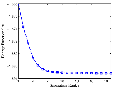
We next demonstrate that the sequence of separated approximations of the form (25) generated by the ARR algorithm results in a non-increasing sequence of π𝜋\pi in 𝒖1subscript𝒖1\bm{u}_{1} and 𝒖2subscript𝒖2\bm{u}_{2}, and a non-decreasing sequence of π𝜋\pi in 𝝀𝝀\bm{\lambda}. In other words, the ARR algorithm iteratively improves the approximation to the saddle point problem (16) unless 𝒖1subscript𝒖1\bm{u}_{1}, 𝒖2subscript𝒖2\bm{u}_{2}, or 𝝀𝝀\bm{\lambda} does not change throughout the iterations. In the latter scenario, either the separation rank r𝑟r needs to be increased or the separated approximation has converged to the solution of (16).

Proposition 1 (Iterative improvement of separated representation).

Let (𝐮1(k),𝐮2(k),𝛌(k))superscriptsubscript𝐮1𝑘superscriptsubscript𝐮2𝑘superscript𝛌𝑘(\bm{u}_{1}^{(k)},\bm{u}_{2}^{(k)},\bm{\lambda}^{(k)}) and (𝐮1(k+1),𝐮2(k+1),𝛌(k+1))superscriptsubscript𝐮1𝑘1superscriptsubscript𝐮2𝑘1superscript𝛌𝑘1(\bm{u}_{1}^{(k+1)},\bm{u}_{2}^{(k+1)},\bm{\lambda}^{(k+1)}) be the rank r𝑟r separated representation of the solution (𝐮1,𝐮2,𝛌)subscript𝐮1subscript𝐮2𝛌(\bm{u}_{1},\bm{u}_{2},\bm{\lambda}) after k𝑘k and k+1𝑘1k+1, respectively, ARR updates (37), (40), and (42). Then,

π(𝒖1(k+1),𝒖2(k+1),𝝀(k))π(𝒖1(k),𝒖2(k),𝝀(k))π(𝒖1(k),𝒖2(k),𝝀(k+1)).𝜋superscriptsubscript𝒖1𝑘1superscriptsubscript𝒖2𝑘1superscript𝝀𝑘𝜋superscriptsubscript𝒖1𝑘superscriptsubscript𝒖2𝑘superscript𝝀𝑘𝜋superscriptsubscript𝒖1𝑘superscriptsubscript𝒖2𝑘superscript𝝀𝑘1\pi(\bm{u}_{1}^{(k+1)},\bm{u}_{2}^{(k+1)},\bm{\lambda}^{(k)})\leq\pi(\bm{u}_{1}^{(k)},\bm{u}_{2}^{(k)},\bm{\lambda}^{(k)})\leq\pi(\bm{u}_{1}^{(k)},\bm{u}_{2}^{(k)},\bm{\lambda}^{(k+1)}). (44)
Proof.

We first note that the updates (40) and (42) along 𝝃1subscript𝝃1\bm{\xi}_{1} and 𝝃2subscript𝝃2\bm{\xi}_{2} directions, respectively, lead only to minimizations of π𝜋\pi, see A.2. Additionally, 𝒖^0,1subscript^𝒖01\hat{\bm{u}}_{0,1} and 𝒖^0,2subscript^𝒖02\hat{\bm{u}}_{0,2} (or equivalently, {𝒖0,1l}l=1rsuperscriptsubscriptsuperscriptsubscript𝒖01𝑙𝑙1𝑟\{\bm{u}_{0,1}^{l}\}_{l=1}^{r} and {𝒖0,2l}l=1rsuperscriptsubscriptsuperscriptsubscript𝒖02𝑙𝑙1𝑟\{\bm{u}_{0,2}^{l}\}_{l=1}^{r}) in (37) are obtained by minimizing π𝜋\pi, thus implying the left inequality in (44). Finally, the right inequality in (44) holds as π𝜋\pi may increase only through the updates 𝝀^0subscript^𝝀0\hat{\bm{\lambda}}_{0} in (37). ∎

The ARR algorithm is summarized in Algorithm 1.

Algorithm 1 Alternating Rayleigh-Ritz (ARR) Algorithm
1:  \bullet Input: target accuracy ϵitalic-ϵ\epsilon
2:  \bullet Output: separation rank r𝑟r, {𝒖0,1l}l=1rsuperscriptsubscriptsuperscriptsubscript𝒖01𝑙𝑙1𝑟\{\bm{u}_{0,1}^{l}\}_{l=1}^{r}, {𝒖0,2l}l=1rsuperscriptsubscriptsuperscriptsubscript𝒖02𝑙𝑙1𝑟\{\bm{u}_{0,2}^{l}\}_{l=1}^{r}, {𝝀0l}l=1rsuperscriptsubscriptsuperscriptsubscript𝝀0𝑙𝑙1𝑟\{\bm{\lambda}_{0}^{l}\}_{l=1}^{r}, {ϕ1l}l=1rsuperscriptsubscriptsuperscriptsubscriptitalic-ϕ1𝑙𝑙1𝑟\{\phi_{1}^{l}\}_{l=1}^{r}, and {ϕ2l}l=1rsuperscriptsubscriptsuperscriptsubscriptitalic-ϕ2𝑙𝑙1𝑟\{\phi_{2}^{l}\}_{l=1}^{r}
3:  \bullet Set r=1𝑟1r=1; (randomly) initialize ϕ11superscriptsubscriptitalic-ϕ11\phi_{1}^{1} and ϕ21superscriptsubscriptitalic-ϕ21\phi_{2}^{1}
4:  while ϵresr>ϵsuperscriptsubscriptitalic-ϵ𝑟𝑒𝑠𝑟italic-ϵ{\epsilon_{res}^{r}}>\epsilon do
5:     while π𝜋\pi changes more than some tolerance tolr𝑡𝑜subscript𝑙𝑟tol_{r} do
6:        \bullet Update {𝒖0,1l}l=1rsuperscriptsubscriptsuperscriptsubscript𝒖01𝑙𝑙1𝑟\{\bm{u}_{0,1}^{l}\}_{l=1}^{r}, {𝒖0,2l}l=1rsuperscriptsubscriptsuperscriptsubscript𝒖02𝑙𝑙1𝑟\{\bm{u}_{0,2}^{l}\}_{l=1}^{r}, and {𝝀0l}l=1rsuperscriptsubscriptsuperscriptsubscript𝝀0𝑙𝑙1𝑟\{\bm{\lambda}_{0}^{l}\}_{l=1}^{r} by solving (37)
7:        \bullet Update {ϕ1l}l=1rsuperscriptsubscriptsuperscriptsubscriptitalic-ϕ1𝑙𝑙1𝑟\{\phi_{1}^{l}\}_{l=1}^{r} by solving (40)
8:        \bullet Update {ϕ2l}l=1rsuperscriptsubscriptsuperscriptsubscriptitalic-ϕ2𝑙𝑙1𝑟\{\phi_{2}^{l}\}_{l=1}^{r} by solving (42)
9:     end while
10:     \bullet Compute the residual error ϵresrsuperscriptsubscriptitalic-ϵ𝑟𝑒𝑠𝑟{\epsilon_{res}^{r}}
11:     \bullet Set r=r+1𝑟𝑟1{r=r+1}; (randomly) initialize ϕ1rsuperscriptsubscriptitalic-ϕ1𝑟\phi_{1}^{r} and ϕ2rsuperscriptsubscriptitalic-ϕ2𝑟\phi_{2}^{r}
12:  end while
Remark 2.

It is worthwhile noting that the ARR algorithm presented here may be interpreted as a variation of the block Gauss-Seidel or multiplicative Schwarz [54] methods.

To complete our discussion on the ARR algorithm we next present an extension of the classical FETI algorithm to solve the saddle point problem (37).

5.2 FETI solution of saddle point problem (37)

We are interested in parallel solution of (37) such that minimal exchange of information between the sub-domain solvers is required. This may be achieved by, for instance, an extension of the classical FETI method for the particular case of problem (37). This is the approach we take in the present study. FETI, one of the widely used DD approaches, was first introduced by Farhat and Roux [24] for the parallel FE solution of second order, self-adjoint elliptic equations. It has also been successfully extended to many other problems; multiple right-hand sides [26], transient problems [21], plate bending problems [23], and non-linear problems [30]. We stress that, for the sake of simplicity, we use the original FETI [24] approach, but with some extensions one may also utilize more recent versions of FETI such as FETI-DP [22].

The FETI method is a non-overlapping DD scheme based on partitioning the computational domain into a number of sub-domains and enforcing the continuity of the solution across the sub-domain interfaces via Lagrange multipliers. In practice, after partitioning the original domain 𝒟𝒟\mathcal{D}, there might be some sub-domains with insufficient Dirichlet boundary conditions resulting in positive semi-definite sub-domain stiffness matrices. These are also known as floating sub-domains. For a partition consisting of two sub-domains 𝒟1subscript𝒟1\mathcal{D}_{1} and 𝒟2subscript𝒟2\mathcal{D}_{2}, we assume that 𝒟2subscript𝒟2\mathcal{D}_{2} has no Dirichlet boundary condition and is a floating sub-domain with symmetric positive semi-definite stiffness matrix 𝑲2(𝝃2)subscript𝑲2subscript𝝃2\bm{K}_{2}(\bm{\xi}_{2}), while 𝒟1subscript𝒟1\mathcal{D}_{1} is non-floating with symmetric positive definite stiffness matrix 𝑲1(𝝃1)subscript𝑲1subscript𝝃1\bm{K}_{1}(\bm{\xi}_{1}). Therefore, the second equation in (37), i.e.,

𝑲^2𝒖^0,2=𝒇^2𝑪^2𝝀^0,subscript^𝑲2subscript^𝒖02subscript^𝒇2subscript^𝑪2subscript^𝝀0\displaystyle\hat{\bm{K}}_{2}\hat{\bm{u}}_{0,2}=\hat{\bm{f}}_{2}-\hat{\bm{C}}_{2}\hat{\bm{\lambda}}_{0}, (45)

is solvable if and only if, [24],

𝑹^2(𝒇^2𝑪^2𝝀^0)=𝟎,subscript^𝑹2subscript^𝒇2subscript^𝑪2subscript^𝝀00\hat{\bm{R}}_{2}\left(\hat{\bm{f}}_{2}-\hat{\bm{C}}_{2}\hat{\bm{\lambda}}_{0}\right)=\bm{0}, (46)

where 𝑹^2subscript^𝑹2\hat{\bm{R}}_{2} spans the null space of 𝑲^2subscript^𝑲2\hat{\bm{K}}_{2}, i.e., range(𝑹^2)=ker(𝑲^2)rangesubscript^𝑹2kersubscript^𝑲2\mathrm{range}(\hat{\bm{R}}_{2})=\mathrm{ker}(\hat{\bm{K}}_{2}). In Section 5.2.1 we will discuss how 𝑹^2subscript^𝑹2\hat{\bm{R}}_{2} is set in our formulation. The solution of (37) can then be written as

(𝑪^1T𝑲^11𝑪^1+𝑪^2T𝑲^2+𝑪^2)𝝀^0=𝑪^1T𝑲^11𝒇^1+𝑪^2T(𝑲^2+𝒇^2+𝑹^2𝜶^0),superscriptsubscript^𝑪1𝑇superscriptsubscript^𝑲11subscript^𝑪1superscriptsubscript^𝑪2𝑇superscriptsubscript^𝑲2subscript^𝑪2subscript^𝝀0superscriptsubscript^𝑪1𝑇superscriptsubscript^𝑲11subscript^𝒇1superscriptsubscript^𝑪2𝑇superscriptsubscript^𝑲2subscript^𝒇2subscript^𝑹2subscript^𝜶0\displaystyle\left(\hat{\bm{C}}_{1}^{T}\hat{\bm{K}}_{1}^{-1}\hat{\bm{C}}_{1}+\hat{\bm{C}}_{2}^{T}\hat{\bm{K}}_{2}^{+}\hat{\bm{C}}_{2}\right)\hat{\bm{\lambda}}_{0}=-\hat{\bm{C}}_{1}^{T}\hat{\bm{K}}_{1}^{-1}\hat{\bm{f}}_{1}+\hat{\bm{C}}_{2}^{T}\left(\hat{\bm{K}}_{2}^{+}\hat{\bm{f}}_{2}+\hat{\bm{R}}_{2}\hat{\bm{\alpha}}_{0}\right),
𝒖^0,1=𝑲^11(𝒇^1𝑪^1𝝀^0),subscript^𝒖01superscriptsubscript^𝑲11subscript^𝒇1subscript^𝑪1subscript^𝝀0\displaystyle\hat{\bm{u}}_{0,1}=\hat{\bm{K}}_{1}^{-1}\left(\hat{\bm{f}}_{1}-\hat{\bm{C}}_{1}\hat{\bm{\lambda}}_{0}\right),
𝒖^0,2=𝑲^2+(𝒇^2𝑪^2𝝀^0)+𝑹^2𝜶^0,subscript^𝒖02superscriptsubscript^𝑲2subscript^𝒇2subscript^𝑪2subscript^𝝀0subscript^𝑹2subscript^𝜶0\displaystyle\hat{\bm{u}}_{0,2}=\hat{\bm{K}}_{2}^{+}\left(\hat{\bm{f}}_{2}-\hat{\bm{C}}_{2}\hat{\bm{\lambda}}_{0}\right)+\hat{\bm{R}}_{2}\hat{\bm{\alpha}}_{0}, (47)

where 𝑲^11superscriptsubscript^𝑲11\hat{\bm{K}}_{1}^{-1} and 𝑲^2+superscriptsubscript^𝑲2\hat{\bm{K}}_{2}^{+} are the inverse and pseudo-inverse of 𝑲^1subscript^𝑲1\hat{\bm{K}}_{1} and 𝑲^2subscript^𝑲2\hat{\bm{K}}_{2}, respectively. Here, 𝜶^0subscript^𝜶0\hat{\bm{\alpha}}_{0} is an unknown vector of coefficients. As it can be seen, there are four unknowns in (5.2) while only three equations are available. The orthogonality condition in (46) is the fourth equation which makes (5.2) determined. We can write the FETI interface problem by combining (46) and the first equation in (5.2) as

[𝑭^I𝑹^2I𝑹^2IT𝟎]{𝝀^𝜶^0}={𝒅^𝒆^},delimited-[]subscript^𝑭𝐼superscriptsubscript^𝑹2𝐼superscriptsubscript^𝑹2superscript𝐼𝑇0^𝝀subscript^𝜶0^𝒅^𝒆\left[\begin{array}[]{cc}\hat{\bm{F}}_{I}&-\hat{\bm{R}}_{2}^{I}\\ -\hat{\bm{R}}_{2}^{I^{T}}&\bm{0}\end{array}\right]\left\{\begin{array}[]{c}\hat{\bm{\lambda}}\\ \hat{\bm{\alpha}}_{0}\end{array}\right\}=\left\{\begin{array}[]{c}\hat{\bm{d}}\\ -\hat{\bm{e}}\end{array}\right\}, (48)

where

𝑭^I=𝑪^1T𝑲^11𝑪^1+𝑪^2T𝑲^2+𝑪^2,subscript^𝑭𝐼superscriptsubscript^𝑪1𝑇superscriptsubscript^𝑲11subscript^𝑪1superscriptsubscript^𝑪2𝑇superscriptsubscript^𝑲2subscript^𝑪2\displaystyle\hat{\bm{F}}_{I}=\hat{\bm{C}}_{1}^{T}\hat{\bm{K}}_{1}^{-1}\hat{\bm{C}}_{1}+\hat{\bm{C}}_{2}^{T}\hat{\bm{K}}_{2}^{+}\hat{\bm{C}}_{2},
𝑹^2I=𝑪^2T𝑹^2,superscriptsubscript^𝑹2𝐼superscriptsubscript^𝑪2𝑇subscript^𝑹2\displaystyle\hat{\bm{R}}_{2}^{I}=\hat{\bm{C}}_{2}^{T}\hat{\bm{R}}_{2},
𝒅^=𝑪^2T𝑲^2+𝒇^2𝑪^1T𝑲^11𝒇^1,^𝒅superscriptsubscript^𝑪2𝑇superscriptsubscript^𝑲2subscript^𝒇2superscriptsubscript^𝑪1𝑇superscriptsubscript^𝑲11subscript^𝒇1\displaystyle\hat{\bm{d}}=\hat{\bm{C}}_{2}^{T}\hat{\bm{K}}_{2}^{+}\hat{\bm{f}}_{2}-\hat{\bm{C}}_{1}^{T}\hat{\bm{K}}_{1}^{-1}\hat{\bm{f}}_{1},
𝒆^=𝑹^2T𝒇^2.^𝒆superscriptsubscript^𝑹2𝑇subscript^𝒇2\displaystyle\hat{\bm{e}}=\hat{\bm{R}}_{2}^{T}\hat{\bm{f}}_{2}. (49)

The solution to (37) can then be obtained by first solving the interface problem (48) for 𝝀^^𝝀\hat{\bm{\lambda}} and 𝜶^0subscript^𝜶0\hat{\bm{\alpha}}_{0} and then by substituting these into the last two equations in (5.2) to compute 𝒖^0,1subscript^𝒖01\hat{\bm{u}}_{0,1} and 𝒖^0,2subscript^𝒖02\hat{\bm{u}}_{0,2}. In order to avoid an explicit assembly of 𝑭^Isubscript^𝑭𝐼\hat{\bm{F}}_{I} in (48), the preconditioned conjugate projected gradient (PCPG) algorithm of [24], which utilizes matrix-vector products, may be extended to compute 𝝀^^𝝀\hat{\bm{\lambda}} in (48). Algorithm 2 summarizes steps of PCPG solver, in which ϵPCPGsubscriptitalic-ϵ𝑃𝐶𝑃𝐺\epsilon_{PCPG} is a stopping criterion, 𝑷^=𝑰𝑹^2I(𝑹^2IT𝑹^2I)1𝑹^2IT^𝑷𝑰superscriptsubscript^𝑹2𝐼superscriptsuperscriptsubscript^𝑹2superscript𝐼𝑇superscriptsubscript^𝑹2𝐼1superscriptsubscript^𝑹2superscript𝐼𝑇\hat{\bm{P}}=\bm{I}-\hat{\bm{R}}_{2}^{I}(\hat{\bm{R}}_{2}^{I^{T}}\hat{\bm{R}}_{2}^{I})^{-1}\hat{\bm{R}}_{2}^{I^{T}} is an orthogonal projection onto the null space of 𝑹^2Isuperscriptsubscript^𝑹2𝐼\hat{\bm{R}}_{2}^{I}, 𝑰𝑰\bm{I} is the identity matrix of size rMI×rMI𝑟subscript𝑀𝐼𝑟subscript𝑀𝐼rM_{I}\times rM_{I}, and 𝑭¯I1superscriptsubscript¯𝑭𝐼1\bar{\bm{F}}_{I}^{-1} is a suitable preconditioner. For a detailed description of the PCPG solver and different choices of preconditioners we refer the interested reader to [53, 37, 58, 52, 27, 12]. In the numerical result of Section 6.2, we have adopted the preconditioner 𝑭¯I1superscriptsubscript¯𝑭𝐼1\bar{\bm{F}}_{I}^{-1} proposed in [37]. An optimal selection or design of 𝑭¯I1superscriptsubscript¯𝑭𝐼1\bar{\bm{F}}_{I}^{-1}, however, requires further study.

After computing 𝝀^^𝝀\hat{\bm{\lambda}}, we obtain 𝜶^0subscript^𝜶0\hat{\bm{\alpha}}_{0} from

𝜶^0=(𝑹^2IT𝑹^2I)1𝑹^2IT(𝑭^I𝝀^𝒅^).subscript^𝜶0superscriptsuperscriptsubscript^𝑹2superscript𝐼𝑇superscriptsubscript^𝑹2𝐼1superscriptsubscript^𝑹2superscript𝐼𝑇subscript^𝑭𝐼^𝝀^𝒅\displaystyle\hat{\bm{\alpha}}_{0}=(\hat{\bm{R}}_{2}^{I^{T}}\hat{\bm{R}}_{2}^{I})^{-1}\hat{\bm{R}}_{2}^{I^{T}}(\hat{\bm{F}}_{I}\hat{\bm{\lambda}}-\hat{\bm{d}}).
Algorithm 2 The FETI PCPG Algorithm
1:  \bullet Initialize 𝝀^0=𝑹^2I(𝑹^2IT𝑹^2I)1𝑹^2T𝒇^2subscript^𝝀0superscriptsubscript^𝑹2𝐼superscriptsuperscriptsubscript^𝑹2superscript𝐼𝑇superscriptsubscript^𝑹2𝐼1superscriptsubscript^𝑹2𝑇subscript^𝒇2\hat{\bm{\lambda}}_{0}=\hat{\bm{R}}_{2}^{I}(\hat{\bm{R}}_{2}^{I^{T}}\hat{\bm{R}}_{2}^{I})^{-1}\hat{\bm{R}}_{2}^{T}\hat{\bm{f}}_{2}, 𝒘0=𝑷^𝒅^𝑷^𝑭^I𝝀^0subscript𝒘0^𝑷^𝒅^𝑷subscript^𝑭𝐼subscript^𝝀0\bm{w}_{0}=\hat{\bm{P}}\hat{\bm{d}}-\hat{\bm{P}}\hat{\bm{F}}_{I}\hat{\bm{\lambda}}_{0}, k=1𝑘1k=1
2:  while 𝒘k1L2/𝒅^L2ϵPCPGsubscriptnormsubscript𝒘𝑘1subscript𝐿2subscriptnorm^𝒅subscript𝐿2subscriptitalic-ϵ𝑃𝐶𝑃𝐺||\bm{w}_{k-1}||_{L_{2}}/||\hat{\bm{d}}||_{L_{2}}\geqslant\epsilon_{PCPG}  do
3:     \bullet 𝒛k1=𝑭¯I1(𝑷^T𝒘k1)subscript𝒛𝑘1superscriptsubscript¯𝑭𝐼1superscript^𝑷𝑇subscript𝒘𝑘1\bm{z}_{k-1}=\bar{\bm{F}}_{I}^{-1}(\hat{\bm{P}}^{T}\bm{w}_{k-1})
4:     \bullet 𝒚k1=𝑷^𝒛k1subscript𝒚𝑘1^𝑷subscript𝒛𝑘1\bm{y}_{k-1}=\hat{\bm{P}}\bm{z}_{k-1}
5:     \bullet sk=𝒚k1T𝒘k1/𝒚k2T𝒘k2subscript𝑠𝑘superscriptsubscript𝒚𝑘1𝑇subscript𝒘𝑘1superscriptsubscript𝒚𝑘2𝑇subscript𝒘𝑘2{s}_{k}=\bm{y}_{k-1}^{T}\bm{w}_{k-1}/\bm{y}_{k-2}^{T}\bm{w}_{k-2}         (s1=0)subscript𝑠10({s}_{1}=0)
6:     \bullet 𝒑k=𝒚k1+sk𝒑k1subscript𝒑𝑘subscript𝒚𝑘1subscript𝑠𝑘subscript𝒑𝑘1\bm{p}_{k}=\bm{y}_{k-1}+{s}_{k}\bm{p}_{k-1}                (𝒑1=𝒚0)subscript𝒑1subscript𝒚0(\bm{p}_{1}=\bm{y}_{0})
7:     \bullet γk=𝒚k1T𝒘k1/𝒑kT𝑭^I𝒑ksubscript𝛾𝑘superscriptsubscript𝒚𝑘1𝑇subscript𝒘𝑘1superscriptsubscript𝒑𝑘𝑇subscript^𝑭𝐼subscript𝒑𝑘{\gamma}_{k}=\bm{y}_{k-1}^{T}\bm{w}_{k-1}/\bm{p}_{k}^{T}\hat{\bm{F}}_{I}\bm{p}_{k}
8:     \bullet 𝝀^k=𝝀^k1+γk𝒑ksubscript^𝝀𝑘subscript^𝝀𝑘1subscript𝛾𝑘subscript𝒑𝑘\hat{\bm{\lambda}}_{k}=\hat{\bm{\lambda}}_{k-1}+{\gamma}_{k}\bm{p}_{k}
9:     \bullet 𝒘k=𝒘k1γk𝑷^𝑭^I𝒑ksubscript𝒘𝑘subscript𝒘𝑘1subscript𝛾𝑘^𝑷subscript^𝑭𝐼subscript𝒑𝑘{\bm{w}}_{k}={\bm{w}}_{k-1}-{\gamma}_{k}\hat{\bm{P}}\hat{\bm{F}}_{I}\bm{p}_{k}
10:  end while

Next, we propose a method to set 𝑹^2subscript^𝑹2\hat{\bm{R}}_{2} which does not require an explicit computation of the null space of 𝑲^2subscript^𝑲2\hat{\bm{K}}_{2}.

5.2.1 Setting 𝑹^2subscript^𝑹2\hat{\bm{R}}_{2}

Since 𝑲^2subscript^𝑲2\hat{\bm{K}}_{2} is not assembled in practice, we cannot obtain 𝑹^2subscript^𝑹2\hat{\bm{R}}_{2} via a direct null space computation of 𝑲^2subscript^𝑲2\hat{\bm{K}}_{2}. For a deterministic problem, rigid body modes of the physical domain span the null space of the stiffness matrix [24]. For three-dimensional problems, the maximum number of rigid body modes is six, while for two-dimensional deterministic problems this number reduces to three. Let 𝑹2subscript𝑹2{\bm{R}}_{2} denote the matrix associated with the rigid body modes of the sub-domain 𝒟2subscript𝒟2\mathcal{D}_{2} computed based on the geometry of 𝒟2subscript𝒟2\mathcal{D}_{2}, see, e.g. [50]. Then 𝑹^2subscript^𝑹2\hat{\bm{R}}_{2} may be set as follows.

Proposition 2.

𝑹^2subscript^𝑹2\hat{\bm{R}}_{2} is an r×r𝑟𝑟r\times r block diagonal matrix whose (l,l)𝑙𝑙(l,l) block, l=1,,r𝑙1𝑟l=1,\cdots,r, is given by

𝑹^2(l,l)=𝑹2.subscript^𝑹2𝑙𝑙subscript𝑹2\hat{\bm{R}}_{2}(l,l)={\bm{R}}_{2}. (50)
Proof.

Since columns of 𝑹2subscript𝑹2{\bm{R}}_{2} are linearly independent, columns of 𝑹^2subscript^𝑹2\hat{\bm{R}}_{2} are also linearly independent as 𝑹^2subscript^𝑹2\hat{\bm{R}}_{2} is block diagonal. On the other hand, as the columns of 𝑹2subscript𝑹2{\bm{R}}_{2} form a basis for the null space of 𝑲2(𝝃)subscript𝑲2𝝃\bm{K}_{2}(\bm{\xi}), we have 𝑲^2(l,l)𝑹2=𝟎subscript^𝑲2𝑙𝑙subscript𝑹20\hat{\bm{K}}_{2}(l,l)\bm{R}_{2}=\bm{0}, l=1,,r𝑙1𝑟l=1,\cdots,r, where 𝑲^2(l,l)subscript^𝑲2𝑙𝑙\hat{\bm{K}}_{2}(l,l) is given in (5.1). Consequently 𝑲^2𝑹^2=𝟎subscript^𝑲2subscript^𝑹20\hat{\bm{K}}_{2}\hat{\bm{R}}_{2}=\bm{0}, which, together with the linear independency of the columns of 𝑹^2subscript^𝑹2\hat{\bm{R}}_{2}, implies range(𝑹^2)=ker(𝑲^2)rangesubscript^𝑹2kersubscript^𝑲2\mathrm{range}(\hat{\bm{R}}_{2})=\mathrm{ker}(\hat{\bm{K}}_{2}). ∎

5.3 Response statistics

In this section, the computation of response statistics based on the separated representation (25) is presented. Let us denote the mean and variance of the separated representation 𝒖ir=l=1r𝒖0,ilϕ1lϕ2lsuperscriptsubscript𝒖𝑖𝑟superscriptsubscript𝑙1𝑟superscriptsubscript𝒖0𝑖𝑙superscriptsubscriptitalic-ϕ1𝑙superscriptsubscriptitalic-ϕ2𝑙\bm{u}_{i}^{r}=\sum_{l=1}^{r}\bm{u}_{0,i}^{l}\phi_{1}^{l}\phi_{2}^{l}, i=1,2𝑖12i=1,2, by 𝔼[𝒖ir]𝔼delimited-[]superscriptsubscript𝒖𝑖𝑟\mathbb{E}[\bm{u}_{i}^{r}] and var[𝒖ir]vardelimited-[]superscriptsubscript𝒖𝑖𝑟\mathrm{var}[\bm{u}_{i}^{r}], respectively. For example, we can approximate the point-wise mean and the second moment of the sub-domain solutions 𝒖isubscript𝒖𝑖\bm{u}_{i} by

𝔼[𝒖ir]=l=1r𝒖0,il𝔼𝝃1[ϕ1l]𝔼𝝃2[ϕ2l],𝔼delimited-[]superscriptsubscript𝒖𝑖𝑟superscriptsubscript𝑙1𝑟superscriptsubscript𝒖0𝑖𝑙subscript𝔼subscript𝝃1delimited-[]superscriptsubscriptitalic-ϕ1𝑙subscript𝔼subscript𝝃2delimited-[]superscriptsubscriptitalic-ϕ2𝑙\displaystyle\mathbb{E}[\bm{u}_{i}^{r}]=\sum_{l=1}^{r}\bm{u}_{0,i}^{l}\mathbb{E}_{\bm{\xi}_{1}}[\phi_{1}^{l}]\mathbb{E}_{\bm{\xi}_{2}}[\phi_{2}^{l}],
𝔼[𝒖ir𝒖ir]=l=1rl=1r(𝒖0,il𝒖0,il)𝔼𝝃1[ϕ1lϕ1l]𝔼𝝃2[ϕ2lϕ2l],𝔼delimited-[]superscriptsubscript𝒖𝑖𝑟superscriptsubscript𝒖𝑖𝑟superscriptsubscript𝑙1𝑟superscriptsubscriptsuperscript𝑙1𝑟superscriptsubscript𝒖0𝑖𝑙superscriptsubscript𝒖0𝑖superscript𝑙subscript𝔼subscript𝝃1delimited-[]superscriptsubscriptitalic-ϕ1𝑙superscriptsubscriptitalic-ϕ1superscript𝑙subscript𝔼subscript𝝃2delimited-[]superscriptsubscriptitalic-ϕ2𝑙superscriptsubscriptitalic-ϕ2superscript𝑙\displaystyle\mathbb{E}[\bm{u}_{i}^{r}\circ\bm{u}_{i}^{r}]=\sum_{l=1}^{r}\sum_{l^{\prime}=1}^{r}(\bm{u}_{0,i}^{l}\circ\bm{u}_{0,i}^{l^{\prime}})\mathbb{E}_{\bm{\xi}_{1}}[\phi_{1}^{l}\phi_{1}^{l^{\prime}}]\mathbb{E}_{\bm{\xi}_{2}}[\phi_{2}^{l}\phi_{2}^{l^{\prime}}], (51)

respectively, where \circ denotes the Hadamard product of two vectors. The variance of 𝒖irsuperscriptsubscript𝒖𝑖𝑟\bm{u}_{i}^{r} can then be obtained from var[𝒖ir]=𝔼[𝒖ir𝒖ir]𝔼[𝒖ir]𝔼[𝒖ir]vardelimited-[]superscriptsubscript𝒖𝑖𝑟𝔼delimited-[]superscriptsubscript𝒖𝑖𝑟superscriptsubscript𝒖𝑖𝑟𝔼delimited-[]superscriptsubscript𝒖𝑖𝑟𝔼delimited-[]superscriptsubscript𝒖𝑖𝑟\mathrm{var}[\bm{u}_{i}^{r}]=\mathbb{E}[\bm{u}_{i}^{r}\circ\bm{u}_{i}^{r}]-\mathbb{E}[\bm{u}_{i}^{r}]\circ\mathbb{E}[\bm{u}_{i}^{r}].

Alternatively, one may generate Monte Carlo estimates of the statistics of 𝒖irsuperscriptsubscript𝒖𝑖𝑟\bm{u}_{i}^{r} by directly sampling the representation (25). We use the latter approach to compute the probability density function of the solution of interest in our numerical experiments.

6 Numerical Examples

In this section, we present two numerical examples for the verification of the proposed stochastic coupling framework. In the first example, we consider a linear elliptic PDE defined on a two-dimensional L-shaped (spatial) domain with random diffusion coefficient. The second example deals with the problem of deformation of a linear elastic cantilever beam with uncertain Young’s modulus. In both cases, the uncertainly is represented by random fields taking statistically independent values on two non-overlapping sub-domains. To study the convergence of the separated representation on the entire domain, the mean and standard deviation (std) error measures

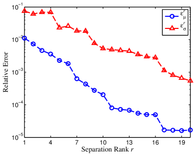
ϵμr=𝔼[𝒖ref]𝔼[𝒖r]L2(M)𝔼[𝒖ref]L2(M)andϵσr=std[𝒖ref]std[𝒖r]L2(M)std[𝒖ref]L2(M)superscriptsubscriptitalic-ϵ𝜇𝑟subscriptnorm𝔼delimited-[]subscript𝒖𝑟𝑒𝑓𝔼delimited-[]superscript𝒖𝑟subscript𝐿2superscript𝑀subscriptnorm𝔼delimited-[]subscript𝒖𝑟𝑒𝑓subscript𝐿2superscript𝑀andsuperscriptsubscriptitalic-ϵ𝜎𝑟subscriptnormstddelimited-[]subscript𝒖𝑟𝑒𝑓stddelimited-[]superscript𝒖𝑟subscript𝐿2superscript𝑀subscriptnormstddelimited-[]subscript𝒖𝑟𝑒𝑓subscript𝐿2superscript𝑀{\epsilon_{\mu}^{r}}=\frac{\big{\|}\mathbb{E}[\bm{u}_{ref}]-\mathbb{E}[\bm{u}^{r}]\big{\|}_{L_{2}(\mathbb{R}^{M})}}{\big{\|}\mathbb{E}[\bm{u}_{ref}]\big{\|}_{L_{2}(\mathbb{R}^{M})}}\;\;\mathrm{and}\;\;{\epsilon_{\sigma}^{r}}=\frac{\big{\|}\mathrm{std}[\bm{u}_{ref}]-\mathrm{std}[\bm{u}^{r}]\big{\|}_{L_{2}(\mathbb{R}^{M})}}{\big{\|}\mathrm{std}[\bm{u}_{ref}]\big{\|}_{L_{2}(\mathbb{R}^{M})}} (52)

are used. Here 𝒖rsuperscript𝒖𝑟\bm{u}^{r} is the rank r𝑟r separated representation of the solution 𝒖𝒖\bm{u} to the coupled problem (16) and 𝒖refsubscript𝒖𝑟𝑒𝑓\bm{u}_{ref} is the solution to the original problem (5). The reference solution 𝒖refsubscript𝒖𝑟𝑒𝑓\bm{u}_{ref} is the PC expansion of 𝒖𝒖\bm{u} constructed with respect to all random inputs 𝝃𝝃\bm{\xi}. The PC coefficients were computed via least-squares regression using sufficiently large numbers of random realizations of 𝒖𝒖\bm{u}.

6.1 Example I: 2D elliptic PDE with random diffusion coefficient

Consider the following elliptic PDE with random diffusion coefficient κ𝜅\kappa,

(κ(𝒙,𝝃)u(𝒙,𝝃))=f(𝒙)𝒙𝒟,formulae-sequence𝜅𝒙𝝃𝑢𝒙𝝃𝑓𝒙𝒙subscript𝒟,\displaystyle-\nabla\cdot\left(\kappa(\bm{x},\bm{\xi})\nabla u(\bm{x},\bm{\xi})\right)=f(\bm{x})\qquad\bm{x}\in\mathcal{D}_{,}
u(𝒙,𝝃)=0𝒙𝒟(D),formulae-sequence𝑢𝒙𝝃0𝒙superscript𝒟𝐷\displaystyle u(\bm{x},\bm{\xi})=0\qquad\qquad\qquad\qquad\qquad\ \ \bm{x}\in\partial\mathcal{D}^{(D)},
u(𝒙,𝝃)𝒏=0𝒙𝒟(N),formulae-sequence𝑢𝒙𝝃𝒏0𝒙superscript𝒟𝑁\displaystyle\nabla u(\bm{x},\bm{\xi})\cdot\bm{n}=0\qquad\qquad\qquad\qquad\ \bm{x}\in\partial\mathcal{D}^{(N)}, (53)

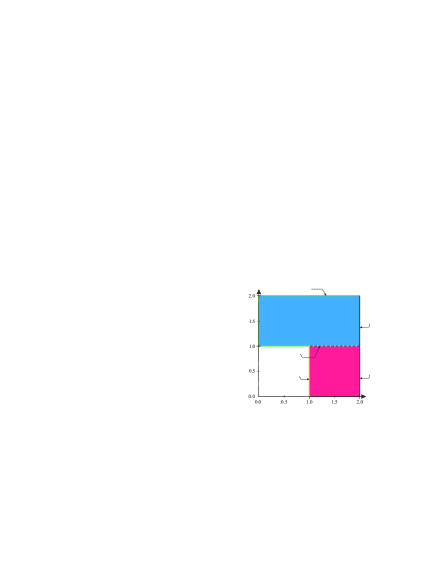
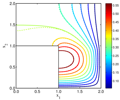
defined over an L-shaped domain 𝒟𝒟\mathcal{D} depicted in Fig. 2. Dirichlet and Neumann boundary conditions are denoted by 𝒟(D)superscript𝒟𝐷\partial\mathcal{D}^{(D)} and 𝒟(N)superscript𝒟𝑁\partial\mathcal{D}^{(N)}, respectively, and 𝒏𝒏\bm{n} is the unit normal vector to 𝒟(N)superscript𝒟𝑁\partial\mathcal{D}^{(N)}.

Refer to caption

𝒟2subscript𝒟2\mathcal{D}_{2}𝒟1subscript𝒟1\mathcal{D}_{1}𝒟1(D)superscriptsubscript𝒟1𝐷\partial\mathcal{D}_{1}^{(D)}𝒟2(D)superscriptsubscript𝒟2𝐷\partial\mathcal{D}_{2}^{(D)}𝒟1(N)superscriptsubscript𝒟1𝑁\partial\mathcal{D}_{1}^{(N)}𝒟2(N)superscriptsubscript𝒟2𝑁\partial\mathcal{D}_{2}^{(N)}ΓIsubscriptΓ𝐼\Gamma_{I}x1subscript𝑥1x_{1}x2subscript𝑥2x_{2}

Figure 2: Geometry of the 2D elliptic problem over an L-shaped domain (𝒟=𝒟1𝒟2𝒟subscript𝒟1subscript𝒟2\mathcal{D}=\mathcal{D}_{1}\cup\mathcal{D}_{2} and 𝒟1𝒟2=subscript𝒟1subscript𝒟2\mathcal{D}_{1}\cap\mathcal{D}_{2}=\emptyset).

We assume 𝒟𝒟\mathcal{D} is composed of two non-overlapping sub-domains 𝒟1subscript𝒟1\mathcal{D}_{1} and 𝒟2subscript𝒟2\mathcal{D}_{2}, i.e., 𝒟=𝒟1𝒟2𝒟subscript𝒟1subscript𝒟2\mathcal{D}=\mathcal{D}_{1}\cup\mathcal{D}_{2} and 𝒟1𝒟2=subscript𝒟1subscript𝒟2\mathcal{D}_{1}\cap\mathcal{D}_{2}=\emptyset on which κ𝜅\kappa and f𝑓f take different values. Specifically, we set

log(κ(𝒙,𝝃)κ0)={G1(𝒙,𝝃1)𝒙𝒟1G2(𝒙,𝝃2)𝒙𝒟2𝜅𝒙𝝃subscript𝜅0casessubscript𝐺1𝒙subscript𝝃1𝒙subscript𝒟1subscript𝐺2𝒙subscript𝝃2𝒙subscript𝒟2\log\left(\kappa(\bm{x},\bm{\xi})-\kappa_{0}\right)=\left\{\begin{array}[]{c}G_{1}(\bm{x},\bm{\xi}_{1})\quad\bm{x}\in\mathcal{D}_{1}\\ G_{2}(\bm{x},\bm{\xi}_{2})\quad\bm{x}\in\mathcal{D}_{2}\end{array}\right. (54)

and

f(𝒙)={10𝒙𝒟10𝒙𝒟2,𝑓𝒙cases10𝒙subscript𝒟10𝒙subscript𝒟2f(\bm{x})=\left\{\begin{array}[]{c}10\quad\bm{x}\in\mathcal{D}_{1}\\ 0\ \ \quad\bm{x}\in\mathcal{D}_{2}\end{array}\right.,

where G1subscript𝐺1G_{1} and G2subscript𝐺2G_{2} are statistically independent Gaussian random fields, and κ0subscript𝜅0\kappa_{0} is a small constant to ensure κ𝜅\kappa is bounded away from zero. Therefore, κ𝜅\kappa in (54) is a (shifted) lognormal random field on sub-domains 𝒟1subscript𝒟1\mathcal{D}_{1} and 𝒟2subscript𝒟2\mathcal{D}_{2}. We represent G1subscript𝐺1G_{1} and G2subscript𝐺2G_{2} by the truncated Karhunen-Loève (KL) expansions

Gi(𝒙,𝝃i)=G¯i+j=1diτi,jgi,j(𝒙)ξi,j,i=1,2,formulae-sequencesubscript𝐺𝑖𝒙subscript𝝃𝑖subscript¯𝐺𝑖superscriptsubscript𝑗1subscript𝑑𝑖subscript𝜏𝑖𝑗subscript𝑔𝑖𝑗𝒙subscript𝜉𝑖𝑗𝑖12G_{i}(\bm{x},\bm{\xi}_{i})=\bar{G}_{i}+\sum_{j=1}^{d_{i}}\sqrt{\tau_{i,j}}g_{i,j}(\bm{x}){\xi}_{i,j},\qquad i=1,2,

where G¯isubscript¯𝐺𝑖\bar{G}_{i} is the mean of Gisubscript𝐺𝑖G_{i}, and {ξ1,j}j=1d1superscriptsubscriptsubscript𝜉1𝑗𝑗1subscript𝑑1\left\{\xi_{1,j}\right\}_{j=1}^{d_{1}} and {ξ2,j}j=1d2superscriptsubscriptsubscript𝜉2𝑗𝑗1subscript𝑑2\left\{\xi_{2,j}\right\}_{j=1}^{d_{2}} are i.i.d. standard Gaussian random variables. Additionally, {τi,j}j=1disuperscriptsubscriptsubscript𝜏𝑖𝑗𝑗1subscript𝑑𝑖\left\{\tau_{i,j}\right\}_{j=1}^{d_{i}} and {gi,j(𝒙)}j=1disuperscriptsubscriptsubscript𝑔𝑖𝑗𝒙𝑗1subscript𝑑𝑖\left\{g_{i,j}(\bm{x})\right\}_{j=1}^{d_{i}} are, respectively, disubscript𝑑𝑖d_{i} largest eigenvalues and the corresponding eigenfunctions of the Gaussian covariance kernel

Ci(𝒙1,𝒙2)=σi2exp(𝒙1𝒙222li2),𝒙1,𝒙2𝒟i.formulae-sequencesubscript𝐶𝑖subscript𝒙1subscript𝒙2superscriptsubscript𝜎𝑖2expsuperscriptsubscriptnormsubscript𝒙1subscript𝒙222superscriptsubscript𝑙𝑖2subscript𝒙1subscript𝒙2subscript𝒟𝑖C_{i}(\bm{x}_{1},\bm{x}_{2})=\sigma_{i}^{2}\mathrm{exp}{\left(-\frac{\|\bm{x}_{1}-\bm{x}_{2}\|_{2}^{2}}{l_{i}^{2}}\right)},\qquad\bm{x}_{1},\bm{x}_{2}\in\mathcal{D}_{i}. (55)

Here, σisubscript𝜎𝑖\sigma_{i} controls the variability of Gisubscript𝐺𝑖G_{i} and lisubscript𝑙𝑖l_{i} is the correlation length of Gisubscript𝐺𝑖G_{i}. To exactly compute the expectations involving 𝑲1(𝝃1)subscript𝑲1subscript𝝃1\bm{K}_{1}(\bm{\xi}_{1}) and 𝑲2(𝝃2)subscript𝑲2subscript𝝃2\bm{K}_{2}(\bm{\xi}_{2}) in (5.1), (5.1), and (5.1), we decompose κ(𝒙,𝝃)𝜅𝒙𝝃\kappa(\bm{x},\bm{\xi}), separately on each sub-domain, into Hermite polynomial chaos of order 2pi2subscript𝑝𝑖2p_{i}, i.e., κ(𝒙,𝝃i)=𝒋di,2piκ𝒋,i(𝒙)ψ𝒋(𝝃i)𝜅𝒙subscript𝝃𝑖subscript𝒋subscriptsubscript𝑑𝑖2subscript𝑝𝑖subscript𝜅𝒋𝑖𝒙subscript𝜓𝒋subscript𝝃𝑖\kappa(\bm{x},\bm{\xi}_{i})=\sum_{\bm{j}\in\mathscr{I}_{d_{i},2p_{i}}}\kappa_{\bm{j},i}(\bm{x})\psi_{\bm{j}}(\bm{\xi}_{i}), 𝒙𝒟i𝒙subscript𝒟𝑖\bm{x}\in\mathcal{D}_{i}. Here, pisubscript𝑝𝑖p_{i} is the order of the PC expansion of the stochastic functions {ϕil(𝝃i)}superscriptsubscriptitalic-ϕ𝑖𝑙subscript𝝃𝑖\{\phi_{i}^{l}(\bm{\xi}_{i})\} in (5.1). For the case of lognormal κ(𝒙,𝝃i)𝜅𝒙subscript𝝃𝑖\kappa(\bm{x},\bm{\xi}_{i}), the expansion coefficients {κ𝒋,i(𝒙)}𝒋di,2pisubscriptsubscript𝜅𝒋𝑖𝒙𝒋subscriptsubscript𝑑𝑖2subscript𝑝𝑖\{\kappa_{\bm{j},i}(\bm{x})\}_{\bm{j}\in\mathscr{I}_{d_{i},2p_{i}}} are available analytically, see [59] or B.

Table 1 summarizes the parameter values involved in the representation of κ𝜅\kappa.

Table 1: Assumed parameters for the PC representation of κ𝜅\kappa in (54).
d1subscript𝑑1d_{1} d2subscript𝑑2d_{2} p1subscript𝑝1p_{1} p2subscript𝑝2p_{2} lc,1subscript𝑙𝑐1l_{c,1} lc,2subscript𝑙𝑐2l_{c,2} G¯¯𝐺\bar{G} σ1subscript𝜎1\sigma_{1} σ2subscript𝜎2\sigma_{2} κ0subscript𝜅0\kappa_{0}
4 6 3 3 2/3 1/3 1 1/2121/2 1/2121/2 0.28
Refer to caption Refer to caption
(a) (b)
Figure 3: Energy functional π𝜋\pi (a) and relative errors in mean and standard deviation (b) as a function of the separation rank r𝑟r for the L-shaped problem. The errors are evaluated from (52).

The FE discretization of (6.1) on each sub-domain is done using the FEniCS package [39]. In particular, we use linear triangle elements with a uniform mesh sizes h1=h2=1/20subscript1subscript2120h_{1}=h_{2}=1/20 along x1subscript𝑥1x_{1} and x2subscript𝑥2x_{2}.

Refer to caption Refer to caption
(a) (b)
Refer to caption Refer to caption
(c) (d)
Figure 4: Contours of the solution mean and standard deviation obtained with separated representation (solid line) and the reference solution (dotted line) for the L-shaped problem. (a) Mean for r=1𝑟1r=1; (b) Standard deviation for r=1𝑟1r=1; (c) Mean for r=20𝑟20r=20; (d) Standard deviation for r=20𝑟20r=20.
Refer to caption
Figure 5: PDF of u(1.0,0.5)𝑢1.00.5u(1.0,0.5) for the L-shaped problem. A comparison between the rank r𝑟r separated representation and the reference solution.
Refer to caption Refer to caption
(a) (b)
Figure 6: PDFs of the normalized ϕ1rsuperscriptsubscriptitalic-ϕ1𝑟\phi_{1}^{r} and ϕ2rsuperscriptsubscriptitalic-ϕ2𝑟\phi_{2}^{r} in the separated representation of the solution to the L-shaped problem. (a) PDF of the normalized ϕ1rsuperscriptsubscriptitalic-ϕ1𝑟\phi_{1}^{r}, r=1,3,7,12𝑟13712r=1,3,7,12; (b) PDF of the normalized ϕ2rsuperscriptsubscriptitalic-ϕ2𝑟\phi_{2}^{r}, r=1,3,7,12𝑟13712r=1,3,7,12. Each ϕirsuperscriptsubscriptitalic-ϕ𝑖𝑟\phi_{i}^{r} is normalized such that it has unit second moment. The PDF of ϕ21superscriptsubscriptitalic-ϕ21\phi_{2}^{1} is not fully shown here.
Refer to caption
Figure 7: PDFs of the normalized stochastic basis functions ϕ1rϕ2rsuperscriptsubscriptitalic-ϕ1𝑟superscriptsubscriptitalic-ϕ2𝑟\phi_{1}^{r}\phi_{2}^{r}, r=1,3,7,12𝑟13712r=1,3,7,12, for the L-shaped problem. Here each basis function is normalized to have unit second moment.

To demonstrate convergence of the separated representation of the solution u𝑢u to (6.1), we increase the separation rank r𝑟r up to r=20𝑟20r=20. Alternatively, we may prescribe a target accuracy ϵitalic-ϵ\epsilon for the residual norm ϵresrsuperscriptsubscriptitalic-ϵ𝑟𝑒𝑠𝑟\epsilon_{res}^{r} in (27) and identify the corresponding separation rank r𝑟r. In the latter approach, the solution refinement is achieved by decreasing ϵitalic-ϵ\epsilon.

Fig. 3(a) shows the values of the energy functional π𝜋\pi with respect to increments in the separation rank r𝑟r. While this is not generally the case, here an increase in r𝑟r leads to a monotonic reduction in π𝜋\pi. Fig. 3(b) presents the mean and standard deviation errors ϵμrsuperscriptsubscriptitalic-ϵ𝜇𝑟\epsilon_{\mu}^{r} and ϵσrsuperscriptsubscriptitalic-ϵ𝜎𝑟\epsilon_{\sigma}^{r}, respectively, as defined in (52). As can be observed from this figure, there is not monotonicity in the reduction of mean and standard deviation errors as a function of r𝑟r.

In Figs. 4(a)-(b) we display the contours of the solution mean and standard deviation obtained from the separated representation with r=1𝑟1r=1 as well as the reference solution. While approximation of the solution mean may be relatively accurate, the standard deviation has not yet converged with r=1𝑟1r=1. By increasing the separation rank to r=20𝑟20r=20, however, the approximation of these quantities improves considerably as can be observed from Figs. 4(c)-(d).

In Fig. 5, the probability density function (PDF) of the separated representation of solution at (x1,x2)=(1.0,0.5)subscript𝑥1subscript𝑥21.00.5(x_{1},x_{2})=(1.0,0.5) is compared to that of the reference solution. For the case of small separation rank, r=1𝑟1r=1, there is a notable difference between the two PDFs. However, this disagreement reduces considerably as the separation rank is increased to r=20𝑟20r=20.

As discussed in Section 5, the stochastic functions {ϕ1l}l=1rsuperscriptsubscriptsuperscriptsubscriptitalic-ϕ1𝑙𝑙1𝑟\{\phi_{1}^{l}\}_{l=1}^{r} and {ϕ2l}l=1rsuperscriptsubscriptsuperscriptsubscriptitalic-ϕ2𝑙𝑙1𝑟\{\phi_{2}^{l}\}_{l=1}^{r} are not fixed a priori and are computed by iteratively solving for the saddle point of π𝜋\pi. Therefore, their representation is problem-dependent. Fig. 6 presents the PDFs of ϕ1rsuperscriptsubscriptitalic-ϕ1𝑟\phi_{1}^{r} and ϕ2rsuperscriptsubscriptitalic-ϕ2𝑟\phi_{2}^{r} when r=1,3,7,12𝑟13712r=1,3,7,12. As it can be observed, these stochastic functions differ from each other and are not identically distributed. The actual stochastic basis functions in (25) are products of these functions, i.e., ϕ1rϕ2rsuperscriptsubscriptitalic-ϕ1𝑟superscriptsubscriptitalic-ϕ2𝑟\phi_{1}^{r}\phi_{2}^{r}. Fig. 7 shows the PDFs of a number of these basis functions. We note that these basis functions are generally different from the PC basis functions.

6.2 Example II: 2D stochastic linear elasticity

For the second numerical example, we consider the linear elasticity problem,

𝝈(𝒖(𝒙,𝝃))=𝟎𝒙𝒟,formulae-sequence𝝈𝒖𝒙𝝃0𝒙subscript𝒟,\displaystyle-\nabla\cdot\bm{\sigma}\left(\bm{u}(\bm{x},\bm{\xi})\right)=\bm{0}\qquad\qquad\bm{x}\in\mathcal{D}_{,}
𝒖(𝒙,𝝃)=𝟎𝒙𝒟(D),formulae-sequence𝒖𝒙𝝃0𝒙superscript𝒟𝐷\displaystyle\bm{u}(\bm{x},\bm{\xi})=\bm{0}\quad\qquad\qquad\qquad\ \ \ \bm{x}\in\partial\mathcal{D}^{(D)},
𝝈(𝒖(𝒙,𝝃))𝒏=𝒕(𝒙)𝒙𝒟(N),formulae-sequence𝝈𝒖𝒙𝝃𝒏𝒕𝒙𝒙superscript𝒟𝑁\displaystyle\bm{\sigma}\left(\bm{u}(\bm{x},\bm{\xi})\right)\bm{n}=\bm{t}(\bm{x})\qquad\qquad\,\bm{x}\in\partial\mathcal{D}^{(N)}, (56)

describing the deformation of the cantilever beam shown in Fig. 8. Here, 𝒖𝒖\bm{u} denotes the displacement vector field, 𝝈𝝈\bm{\sigma} is the stress tensor, 𝒏𝒏\bm{n} is the unit normal vector to the boundary, and 𝒕𝒕\bm{t} is the traction vector. We assume that 𝒕=(0,0.1)𝒕00.1\bm{t}=(0,-0.1) on the edge corresponding to x2=1.0subscript𝑥21.0x_{2}=1.0 and 𝒕=(0,0)𝒕00\bm{t}=(0,0) elsewhere. The stress tensor 𝝈𝝈\bm{\sigma} is related to the strain tensor 𝒆=(𝒖+𝒖T)/2𝒆𝒖superscript𝒖𝑇2\bm{e}=\left(\nabla\bm{u}+{\nabla\bm{u}}^{T}\right)/2 via the isotropic linear elastic stress-strain relation

Refer to caption

𝒟1subscript𝒟1\mathcal{D}_{1}𝒟2subscript𝒟2\mathcal{D}_{2}ΓIsubscriptΓ𝐼\Gamma_{I}clamped end𝒕𝒕\bm{t}x1subscript𝑥1x_{1}x2subscript𝑥2x_{2}

Figure 8: Geometry of the 2D cantilever beam composed of two non-overlapping sub-domains 𝒟1subscript𝒟1\mathcal{D}_{1} and 𝒟2subscript𝒟2\mathcal{D}_{2}. Young’s moduli of the sub-domain materials are statistically independent random fields.
𝝈=E1+ν(𝒆+ν12νtr(𝒆)𝑰),𝝈𝐸1𝜈𝒆𝜈12𝜈tr𝒆𝑰\bm{\sigma}=\frac{E}{1+\nu}\left(\bm{e}+\frac{\nu}{1-2\nu}\ \mathrm{tr}(\bm{e})\bm{I}\right),

where ν=0.3𝜈0.3\nu=0.3 is the Poisson’s ratio. Here, tr()tr\mathrm{tr}(\cdot) denotes the trace operator of a tensor and 𝑰𝑰\bm{I} is the identity tensor of order two. The Young’s modulus E(𝒙,𝝃)𝐸𝒙𝝃E(\bm{x},\bm{\xi}) is the source of uncertainty in (6.2) and is assumed to take statistically independent values over sub-domains 𝒟1subscript𝒟1\mathcal{D}_{1} and 𝒟2subscript𝒟2\mathcal{D}_{2} shown in Fig. 8. Specifically,

E(𝒙,𝝃)={E1(𝒙,𝝃1)𝒙𝒟1E2(𝒙,𝝃2)𝒙𝒟2,𝐸𝒙𝝃casessubscript𝐸1𝒙subscript𝝃1𝒙subscript𝒟1subscript𝐸2𝒙subscript𝝃2𝒙subscript𝒟2E(\bm{x},\bm{\xi})=\left\{\begin{array}[]{c}E_{1}(\bm{x},\bm{\xi}_{1})\quad\bm{x}\in\mathcal{D}_{1}\\ E_{2}(\bm{x},\bm{\xi}_{2})\quad\bm{x}\in\mathcal{D}_{2}\end{array}\right., (57)

where each Ei(𝒙,𝝃i)subscript𝐸𝑖𝒙subscript𝝃𝑖E_{i}(\bm{x},\bm{\xi}_{i}), i=1,2𝑖12i=1,2, is represented by the series

Ei(𝒙,𝝃i)=E¯i+j=1diτi,jgi,j(𝒙)ξi,j,𝒙𝒟i.formulae-sequencesubscript𝐸𝑖𝒙subscript𝝃𝑖subscript¯𝐸𝑖superscriptsubscript𝑗1subscript𝑑𝑖subscript𝜏𝑖𝑗subscript𝑔𝑖𝑗𝒙subscript𝜉𝑖𝑗𝒙subscript𝒟𝑖E_{i}(\bm{x},\bm{\xi}_{i})=\bar{E}_{i}+\sum_{j=1}^{d_{i}}\sqrt{\tau_{i,j}}g_{i,j}(\bm{x})\xi_{i,j},\qquad\bm{x}\in\mathcal{D}_{i}. (58)

Here, {τi,j}j=1disuperscriptsubscriptsubscript𝜏𝑖𝑗𝑗1subscript𝑑𝑖\left\{\tau_{i,j}\right\}_{j=1}^{d_{i}} and {gi,j(𝒙)}j=1disuperscriptsubscriptsubscript𝑔𝑖𝑗𝒙𝑗1subscript𝑑𝑖\left\{g_{i,j}(\bm{x})\right\}_{j=1}^{d_{i}} are disubscript𝑑𝑖d_{i} largest eigenvalues and the corresponding eigenfunctions of the Gaussian covariance kernel given in (55). We assume that {ξ1,j}j=1d1superscriptsubscriptsubscript𝜉1𝑗𝑗1subscript𝑑1\left\{\xi_{1,j}\right\}_{j=1}^{d_{1}} and {ξ2,j}j=1d2superscriptsubscriptsubscript𝜉2𝑗𝑗1subscript𝑑2\left\{\xi_{2,j}\right\}_{j=1}^{d_{2}} are i.i.d. uniform random variables U(1,1)𝑈11U(-1,1). The list of parameters used in the analyses of this example is given in Table 2. These choices ensure that all realizations of E𝐸E are strictly positive on 𝒟𝒟\mathcal{D}.

Table 2: Assumed parameters for the description of Young’s modulus E𝐸E in (57).
d1subscript𝑑1d_{1} d2subscript𝑑2d_{2} ν𝜈\nu lc,1subscript𝑙𝑐1l_{c,1} lc,2subscript𝑙𝑐2l_{c,2} E¯1subscript¯𝐸1\bar{E}_{1} E¯2subscript¯𝐸2\bar{E}_{2} σ1subscript𝜎1\sigma_{1} σ2subscript𝜎2\sigma_{2}
9 11 0.3 2/3 1/3 100 100 35 35

Similar to the L-shaped problem, FE discretizations are done via the FEniCS project [39] and by using linear triangle elements with a uniform grid size h1=h2=1/10subscript1subscript2110h_{1}=h_{2}=1/10 along x1subscript𝑥1x_{1} and x2subscript𝑥2x_{2} directions. Legendre PC expansions of {ϕ1l}l=1rsuperscriptsubscriptsuperscriptsubscriptitalic-ϕ1𝑙𝑙1𝑟\{\phi_{1}^{l}\}_{l=1}^{r} and {ϕ2l}l=1rsuperscriptsubscriptsuperscriptsubscriptitalic-ϕ2𝑙𝑙1𝑟\{\phi_{2}^{l}\}_{l=1}^{r} with degree p=3𝑝3p=3 were found sufficient for the solution of update equations (40) and (42), respectively.

We note that in the present test case, 𝒟2subscript𝒟2\mathcal{D}_{2} is a floating sub-domain with no Dirichlet boundary conditions; therefore, the PCPG solver described in Section 5.2 is applied to compute the vectors of Lagrange multipliers {𝝀0l}l=1rsuperscriptsubscriptsuperscriptsubscript𝝀0𝑙𝑙1𝑟\{\bm{\lambda}_{0}^{l}\}_{l=1}^{r} in (37). We refer to Algorithm 2 for the implementation details of the PCPG solver. In our computations, we have considered ϵPCPG=108subscriptitalic-ϵ𝑃𝐶𝑃𝐺superscript108\epsilon_{PCPG}=10^{-8} as the stopping criterion for the PCPG solver. The condition number of 𝑭I^^subscript𝑭𝐼\hat{\bm{F}_{I}} determines the number of PCPG iterations and generally increases as a function of the separation rank r𝑟r, hence asking for a preconditioner. Selection of an effective preconditioner 𝑭¯I1superscriptsubscript¯𝑭𝐼1\bar{\bm{F}}_{I}^{-1}, however, is generally a non-trivial task in the FETI approach. Among several existing choices, e.g., [53, 37, 58, 52, 27, 12], we found the preconditioner of [37],

𝑭¯I1=(𝑪^1T𝑪^1+𝑪^2T𝑪^2)1(𝑪^1T𝑲^1𝑪^1+𝑪^2T𝑲^2𝑪^2)(𝑪^1T𝑪^1+𝑪^2T𝑪^2)1,superscriptsubscript¯𝑭𝐼1superscriptsubscriptsuperscriptbold-^𝑪𝑇1subscriptbold-^𝑪1subscriptsuperscriptbold-^𝑪𝑇2subscriptbold-^𝑪21subscriptsuperscriptbold-^𝑪𝑇1subscriptbold-^𝑲1subscriptbold-^𝑪1subscriptsuperscriptbold-^𝑪𝑇2subscriptbold-^𝑲2subscriptbold-^𝑪2superscriptsubscriptsuperscriptbold-^𝑪𝑇1subscriptbold-^𝑪1subscriptsuperscriptbold-^𝑪𝑇2subscriptbold-^𝑪21\bar{\bm{F}}_{I}^{-1}=\left(\bm{\hat{C}}^{T}_{1}\bm{\hat{C}}_{1}+\bm{\hat{C}}^{T}_{2}\bm{\hat{C}}_{2}\right)^{-1}\left(\bm{\hat{C}}^{T}_{1}\bm{\hat{K}}_{1}\bm{\hat{C}}_{1}+\bm{\hat{C}}^{T}_{2}\bm{\hat{K}}_{2}\bm{\hat{C}}_{2}\right)\left(\bm{\hat{C}}^{T}_{1}\bm{\hat{C}}_{1}+\bm{\hat{C}}^{T}_{2}\bm{\hat{C}}_{2}\right)^{-1}, (59)

particularly effective for our purpose.
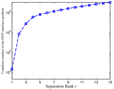
Refer to caption Refer to caption
(a) (b)
Figure 9: Convergence properties of the PCPG algorithm used for the beam problem. (a) Condition number of 𝑭^Isubscript^𝑭𝐼\hat{\bm{F}}_{I} vs. the separation rank; (b) Number of the iterations required for the PCPG algorithm to converge with and without preconditioning vs. the separation rank.

In Fig. 9(a), we show the dependence of the condition number of 𝑭I^^subscript𝑭𝐼\hat{\bm{F}_{I}} on r𝑟r for the present example. A rapid increase in the condition number of 𝑭I^^subscript𝑭𝐼\hat{\bm{F}_{I}} can be observed when r𝑟r is increased. Fig. 9(b) displays the number of PCPG iterations required to reach ϵPCPG=108subscriptitalic-ϵ𝑃𝐶𝑃𝐺superscript108\epsilon_{PCPG}=10^{-8} with the preconditioner (59) and when no preconditioner is used, i.e., 𝑭¯I1=𝑰superscriptsubscript¯𝑭𝐼1𝑰\bar{\bm{F}}_{I}^{-1}=\bm{I}. We observe that the choice of preconditioner (59) makes the convergence of the PCPG solver almost independent of r𝑟r. This is particularly crucial when one is dealing with problems in which r𝑟r is large. However, we note that further analysis is needed to confirm the effectiveness of (59).

Fig. 10 illustrates the convergence of the separated representation. Similar to the L-shaped problem, increasing the separation rank r𝑟r results in a monotonic descries of the energy functional π𝜋\pi, see Fig. 10(a). The relative mean and standard deviation errors ϵμrsuperscriptsubscriptitalic-ϵ𝜇𝑟\epsilon_{\mu}^{r} and ϵσrsuperscriptsubscriptitalic-ϵ𝜎𝑟\epsilon_{\sigma}^{r} of the displacement are computed from (27) and are plotted against r𝑟r in Fig. 10(b).

Refer to caption Refer to caption
(a) (b)
Figure 10: Energy functional π𝜋\pi (a) and relative errors in mean and standard deviation of the displacement (b) as a function of the separation rank r𝑟r for the beam problem. The errors are evaluated from (52).

In Fig. 11, we display the contours of the mean and standard deviation of the vertical displacement obtained from the separated representation, and compare them with those of the reference solution. The mean is captured fairly accurately with a rank one approximation. While for r=1𝑟1r=1 a considerable deviation from the standard deviation of the reference solution is observed, the rank r=15𝑟15r=15 approximation agrees well with the reference solution (Fig. 11(b) and Fig. 11(d)). Despite the high-dimensionality of the solution, i.e., d=20𝑑20d=20, we note that we only require a low separation rank, r=15𝑟15r=15, to accurately approximate the solution mean and standard deviation.

(a) Refer to caption
(b) Refer to caption
(c) Refer to caption
(d) Refer to caption
Figure 11: Contours of the mean and standard deviation of vertical displacement obtained with separated representation (solid line) and the reference solution (dotted line) for the beam problem. (a) Mean for r=1𝑟1r=1; (b) Standard deviation for r=1𝑟1r=1; (c) Mean for r=15𝑟15r=15; (d) Standard deviation for r=15𝑟15r=15.

Fig. 12 compares the PDFs of the separated approximation of the total displacement at (x1,x2)=(5.0,0.0)subscript𝑥1subscript𝑥25.00.0(x_{1},x_{2})=(5.0,0.0), when r=1𝑟1r=1 and r=15𝑟15r=15, to the PDF of the corresponding reference solution. An almost identical agreement between these PDFs is observed when r=15𝑟15r=15.

Refer to caption
Figure 12: PDF of the total displacement at (x1,x2)=(5.0,0.0)subscript𝑥1subscript𝑥25.00.0(x_{1},x_{2})=(5.0,0.0). A comparison between the separated approximation and the reference solution.
Refer to caption Refer to caption
(a) (b)
Figure 13: PDFs of the normalized stochastic functions ϕ1rsuperscriptsubscriptitalic-ϕ1𝑟\phi_{1}^{r} and ϕ2rsuperscriptsubscriptitalic-ϕ2𝑟\phi_{2}^{r}, r=1,3,7,12𝑟13712r=1,3,7,12, for the beam problem. The normalized ϕ1rsuperscriptsubscriptitalic-ϕ1𝑟\phi_{1}^{r} and ϕ2rsuperscriptsubscriptitalic-ϕ2𝑟\phi_{2}^{r} have unit second moment. (a) PDFs of the normalized ϕ1rsuperscriptsubscriptitalic-ϕ1𝑟\phi_{1}^{r}; (b) PDFs of the normalized ϕ2rsuperscriptsubscriptitalic-ϕ2𝑟\phi_{2}^{r}. PDFs of ϕ17superscriptsubscriptitalic-ϕ17\phi_{1}^{7}, ϕ21superscriptsubscriptitalic-ϕ21\phi_{2}^{1}, and ϕ23superscriptsubscriptitalic-ϕ23\phi_{2}^{3} are not shown completely.
Refer to caption
Figure 14: PDFs of the normalized stochastic basis functions ϕ1rϕ2rsuperscriptsubscriptitalic-ϕ1𝑟superscriptsubscriptitalic-ϕ2𝑟\phi_{1}^{r}\phi_{2}^{r}, r=1,3,7,12𝑟13712r=1,3,7,12, for the beam problem. Each ϕ1rϕ2rsuperscriptsubscriptitalic-ϕ1𝑟superscriptsubscriptitalic-ϕ2𝑟\phi_{1}^{r}\phi_{2}^{r} has unit second moment.

To demonstrate that the stochastic functions ϕ1rsuperscriptsubscriptitalic-ϕ1𝑟\phi_{1}^{r} and ϕ2rsuperscriptsubscriptitalic-ϕ2𝑟\phi_{2}^{r} in (25) depend on the problem at hand, we present the PDFs of these quantities, for r=1,3,7,12𝑟13712r=1,3,7,12, in Fig. 13. As it can be seen, these PDFs are different from those of the L-shaped problem. Additionally, Fig. 14 reports the PDF of the stochastic basis functions ϕ1rϕ2rsuperscriptsubscriptitalic-ϕ1𝑟superscriptsubscriptitalic-ϕ2𝑟\phi_{1}^{r}\phi_{2}^{r} for the above r𝑟r values.

7 Conclusion

We have developed a computational framework for the propagation of uncertainty through coupled domain problems. The proposed approach hinges on the construction of a solution-adaptive stochastic basis that is of separated form with respect to the random inputs characterizing the uncertainty in each sub-domain. Such a separated construction of stochastic basis is achieved through a sequence of approximations with respect to the dimensionality, i.e., number of random inputs, of each individual sub-domain and not the combined dimensionality. This leads to a partitioned treatment of the stochastic space and, consequently, a higher scalability of the method as compared with standard uncertainty propagation approaches, such as those based on direct polynomial chaos expansions. For situations where the cardinality of the separated basis – here referred to as the separation rank – is small, the proposed approach provides a reduced order representation of the coupled field solution.

The deterministic coefficients associated with each separated stochastic basis capture the spatial variability of the solution and are computed via the standard finite element tearing and interconnecting (FETI) approach. Therefore, the method achieves a high level of parallelism while requiring no intrusion in each sub-domain solver. Although our present formulation of domain coupling is based on the standard FETI approach, we foresee no major technical difficulties in employing more advanced domain coupling schemes.

The performance of the proposed framework was explored through its application to two linear elliptic PDEs with high-dimensional random inputs. Both problems were defined on physical domains consisting of two coupled sub-domains with independent sources of uncertainty. In both cases, despite the high-dimensionality of the random inputs, accurate estimations of the solution statistics were achieved with relatively low separation ranks, thus demonstrating the effectiveness of the present approach.

The stochastic expansion of this study based on the separated representations may also be applied to other coupled problems, such as fluid structure interaction (FSI), involving uncertainty. However, different numerical strategies for the construction of the separated basis may be required.

Acknowledgements

The authors are indebted to the fruitful discussions they had with Prof. K.C. Park and Prof. Kurt Maute from University of Colorado, Boulder.

AD gratefully acknowledges the financial support of the Department of Energy under Advanced Scientific Computing Research Early Career Research Award DE-SC0006402. MH’s work was supported by the National Science Foundation grant CMMI-1201207. The work of HGM and RN has been partially supported by the Deutsche Forschungsgemeinschaft (DFG) through the SFB 880.

\appendixpage\addappheadtotoc

Appendix A

A.1 Linear system (37) for 𝒖0,1lsuperscriptsubscript𝒖01𝑙\bm{u}_{0,1}^{l}, 𝒖0,2lsuperscriptsubscript𝒖02𝑙\bm{u}_{0,2}^{l}, and 𝝀0lsuperscriptsubscript𝝀0𝑙\bm{\lambda}_{0}^{l} updates

We assume all unknowns are fixed except the vector 𝒖0,1lsuperscriptsubscript𝒖01𝑙\bm{u}_{0,1}^{l}. Taking the derivative of π𝜋\pi in (6) with respect to 𝒖0,1lsuperscriptsubscript𝒖01𝑙\bm{u}_{0,1}^{l}, l=1,,r𝑙1𝑟l=1,\dots,r, leads to the following linear system

l=1r(𝔼[ϕ1lϕ2l𝑲1ϕ1lϕ2l]𝒖0,1l𝔼[ϕ1lϕ2lϕ1lϕ2l]𝑪1𝝀0l)=𝔼[ϕ1lϕ2l𝒇1],l=1,,r.formulae-sequencesuperscriptsubscriptsuperscript𝑙1𝑟𝔼delimited-[]superscriptsubscriptitalic-ϕ1𝑙superscriptsubscriptitalic-ϕ2𝑙subscript𝑲1superscriptsubscriptitalic-ϕ1superscript𝑙superscriptsubscriptitalic-ϕ2superscript𝑙superscriptsubscript𝒖01superscript𝑙𝔼delimited-[]superscriptsubscriptitalic-ϕ1𝑙superscriptsubscriptitalic-ϕ2𝑙superscriptsubscriptitalic-ϕ1superscript𝑙superscriptsubscriptitalic-ϕ2superscript𝑙subscript𝑪1superscriptsubscript𝝀0superscript𝑙𝔼delimited-[]superscriptsubscriptitalic-ϕ1𝑙superscriptsubscriptitalic-ϕ2𝑙subscript𝒇1𝑙1𝑟\sum_{l^{\prime}=1}^{r}\left(\mathbb{E}\left[\phi_{1}^{l}\phi_{2}^{l}\bm{K}_{1}\phi_{1}^{l^{\prime}}\phi_{2}^{l^{\prime}}\right]\bm{u}_{0,1}^{l^{\prime}}-\mathbb{E}\left[\phi_{1}^{l}\phi_{2}^{l}\phi_{1}^{l^{\prime}}\phi_{2}^{l^{\prime}}\right]\bm{C}_{1}\bm{\lambda}_{0}^{l^{\prime}}\right)=\mathbb{E}\left[\phi_{1}^{l}\phi_{2}^{l}\bm{f}_{1}\right],\quad l=1,\dots,r. (60)

Similarly, the 𝒖0,2lsuperscriptsubscript𝒖02𝑙\bm{u}_{0,2}^{l} updates are performed through

l=1r(𝔼[ϕ1lϕ2l𝑲2ϕ1lϕ2l]𝒖0,2l+𝔼[ϕ1lϕ2lϕ1lϕ2l]𝑪2𝝀0l)=𝔼[ϕ1lϕ2l𝒇2],l=1,,r.formulae-sequencesuperscriptsubscriptsuperscript𝑙1𝑟𝔼delimited-[]superscriptsubscriptitalic-ϕ1𝑙superscriptsubscriptitalic-ϕ2𝑙subscript𝑲2superscriptsubscriptitalic-ϕ1superscript𝑙superscriptsubscriptitalic-ϕ2superscript𝑙superscriptsubscript𝒖02superscript𝑙𝔼delimited-[]superscriptsubscriptitalic-ϕ1𝑙superscriptsubscriptitalic-ϕ2𝑙superscriptsubscriptitalic-ϕ1superscript𝑙superscriptsubscriptitalic-ϕ2superscript𝑙subscript𝑪2superscriptsubscript𝝀0superscript𝑙𝔼delimited-[]superscriptsubscriptitalic-ϕ1𝑙superscriptsubscriptitalic-ϕ2𝑙subscript𝒇2𝑙1𝑟\sum_{l^{\prime}=1}^{r}\left(\mathbb{E}\left[\phi_{1}^{l}\phi_{2}^{l}\bm{K}_{2}\phi_{1}^{l^{\prime}}\phi_{2}^{l^{\prime}}\right]\bm{u}_{0,2}^{l^{\prime}}+\mathbb{E}\left[\phi_{1}^{l}\phi_{2}^{l}\phi_{1}^{l^{\prime}}\phi_{2}^{l^{\prime}}\right]\bm{C}_{2}\bm{\lambda}_{0}^{l^{\prime}}\right)=\mathbb{E}\left[\phi_{1}^{l}\phi_{2}^{l}\bm{f}_{2}\right],\quad l=1,\dots,r. (61)

The derivative of π𝜋\pi with respect to deterministic vector 𝝀0lsuperscriptsubscript𝝀0𝑙\bm{\lambda}_{0}^{l} of the Lagrange multipliers satisfies

l=1r(𝔼[ϕ1lϕ2lϕ1lϕ2l]𝑪2T𝒖0,2l𝔼[ϕ1lϕ2lϕ1lϕ2l]𝑪1T𝒖0,1l)=𝟎,l=1,,r.formulae-sequencesuperscriptsubscriptsuperscript𝑙1𝑟𝔼delimited-[]superscriptsubscriptitalic-ϕ1𝑙superscriptsubscriptitalic-ϕ2𝑙superscriptsubscriptitalic-ϕ1superscript𝑙superscriptsubscriptitalic-ϕ2superscript𝑙superscriptsubscript𝑪2𝑇superscriptsubscript𝒖02superscript𝑙𝔼delimited-[]superscriptsubscriptitalic-ϕ1𝑙superscriptsubscriptitalic-ϕ2𝑙superscriptsubscriptitalic-ϕ1superscript𝑙superscriptsubscriptitalic-ϕ2superscript𝑙superscriptsubscript𝑪1𝑇superscriptsubscript𝒖01superscript𝑙0𝑙1𝑟\sum_{l^{\prime}=1}^{r}\left(\mathbb{E}\left[\phi_{1}^{l}\phi_{2}^{l}\phi_{1}^{l^{\prime}}\phi_{2}^{l^{\prime}}\right]\bm{C}_{2}^{T}\bm{u}_{0,2}^{l^{\prime}}-\mathbb{E}\left[\phi_{1}^{l}\phi_{2}^{l}\phi_{1}^{l^{\prime}}\phi_{2}^{l^{\prime}}\right]\bm{C}_{1}^{T}\bm{u}_{0,1}^{l^{\prime}}\right)=\bm{0},\quad l=1,\dots,r. (62)

Putting (60), (61), and (62) together results in the linear system of (37) for 𝒖0,1lsuperscriptsubscript𝒖01𝑙\bm{u}_{0,1}^{l}, 𝒖0,2lsuperscriptsubscript𝒖02𝑙\bm{u}_{0,2}^{l}, and 𝝀0lsuperscriptsubscript𝝀0𝑙\bm{\lambda}_{0}^{l} updates.

A.2 Linear system (42) for ϕ1l(𝝃1)superscriptsubscriptitalic-ϕ1𝑙subscript𝝃1\phi_{1}^{l}(\bm{\xi}_{1}) updates

We first remind that in ϕ1l(𝝃1)superscriptsubscriptitalic-ϕ1𝑙subscript𝝃1\phi_{1}^{l}(\bm{\xi}_{1}) updates the vectors 𝒖0,1lsuperscriptsubscript𝒖01𝑙\bm{u}_{0,1}^{l}, 𝒖0,2lsuperscriptsubscript𝒖02𝑙\bm{u}_{0,2}^{l}, and 𝝀0lsuperscriptsubscript𝝀0𝑙\bm{\lambda}_{0}^{l} are fixed at their current values obtained from (37). As the solution to (37) satisfies the constraints in (62), the term 𝔼[𝝀T(𝑪2T𝒖2𝑪1T𝒖1)]𝔼delimited-[]superscript𝝀𝑇superscriptsubscript𝑪2𝑇subscript𝒖2superscriptsubscript𝑪1𝑇subscript𝒖1\mathbb{E}\left[\bm{\lambda}^{T}\left(\bm{C}_{2}^{T}\bm{u}_{2}-\bm{C}_{1}^{T}\bm{u}_{1}\right)\right] in (6) corresponding to the the interface condition vanishes for any {ϕ1l(𝝃1)}l=1rsuperscriptsubscriptsuperscriptsubscriptitalic-ϕ1𝑙subscript𝝃1𝑙1𝑟\{\phi_{1}^{l}(\bm{\xi}_{1})\}_{l=1}^{r} and {ϕ2l(𝝃2)}l=1rsuperscriptsubscriptsuperscriptsubscriptitalic-ϕ2𝑙subscript𝝃2𝑙1𝑟\{\phi_{2}^{l}(\bm{\xi}_{2})\}_{l=1}^{r}. Therefore, the ϕ1l(𝝃1)superscriptsubscriptitalic-ϕ1𝑙subscript𝝃1\phi_{1}^{l}(\bm{\xi}_{1}) updates correspond to minimization of π𝜋\pi. More precisely, plugging the separated representation (25) into condition (39), we arrive at

(l=1r𝒖l0,1Tϕ2l(𝝃2)𝑲1(𝝃1)𝒖0,1lϕ1l(𝝃1)ϕ2l(𝝃2))δϕ1l(𝝃1)ρ1(𝝃1)d𝝃1ρ2(𝝃2)d𝝃2superscriptsubscriptsuperscript𝑙1𝑟subscriptsuperscriptsuperscript𝒖𝑙𝑇01superscriptsubscriptitalic-ϕ2𝑙subscript𝝃2subscript𝑲1subscript𝝃1superscriptsubscript𝒖01superscript𝑙superscriptsubscriptitalic-ϕ1superscript𝑙subscript𝝃1superscriptsubscriptitalic-ϕ2superscript𝑙subscript𝝃2𝛿superscriptsubscriptitalic-ϕ1𝑙subscript𝝃1subscript𝜌1subscript𝝃1differential-dsubscript𝝃1subscript𝜌2subscript𝝃2differential-dsubscript𝝃2\displaystyle\int\int\left(\sum_{l^{\prime}=1}^{r}{\bm{u}^{l}}^{T}_{0,1}\phi_{2}^{l}(\bm{\xi}_{2})\bm{K}_{1}(\bm{\xi}_{1})\bm{u}_{0,1}^{l^{\prime}}\phi_{1}^{l^{\prime}}(\bm{\xi}_{1})\phi_{2}^{l^{\prime}}(\bm{\xi}_{2})\right)\delta\phi_{1}^{l}(\bm{\xi}_{1})\rho_{1}(\bm{\xi}_{1})\mathrm{d}\bm{\xi}_{1}\rho_{2}(\bm{\xi}_{2})\mathrm{d}\bm{\xi}_{2}
+(l=1r𝒖l0,2Tϕ2l(𝝃2)𝑲2(𝝃2)𝒖0,2lϕ1l(𝝃1)ϕ2l(𝝃2))δϕ1l(𝝃1)ρ1(𝝃1)d𝝃1ρ2(𝝃2)d𝝃2superscriptsubscriptsuperscript𝑙1𝑟subscriptsuperscriptsuperscript𝒖𝑙𝑇02superscriptsubscriptitalic-ϕ2𝑙subscript𝝃2subscript𝑲2subscript𝝃2superscriptsubscript𝒖02superscript𝑙superscriptsubscriptitalic-ϕ1superscript𝑙subscript𝝃1superscriptsubscriptitalic-ϕ2superscript𝑙subscript𝝃2𝛿superscriptsubscriptitalic-ϕ1𝑙subscript𝝃1subscript𝜌1subscript𝝃1differential-dsubscript𝝃1subscript𝜌2subscript𝝃2differential-dsubscript𝝃2\displaystyle+\int\int\left(\sum_{l^{\prime}=1}^{r}{\bm{u}^{l}}^{T}_{0,2}\phi_{2}^{l}(\bm{\xi}_{2})\bm{K}_{2}(\bm{\xi}_{2})\bm{u}_{0,2}^{l^{\prime}}\phi_{1}^{l^{\prime}}(\bm{\xi}_{1})\phi_{2}^{l^{\prime}}(\bm{\xi}_{2})\right)\delta\phi_{1}^{l}(\bm{\xi}_{1})\rho_{1}(\bm{\xi}_{1})\mathrm{d}\bm{\xi}_{1}\rho_{2}(\bm{\xi}_{2})\mathrm{d}\bm{\xi}_{2}
=(𝒖l0,1T𝒇1ϕ2l(𝝃2)+𝒖l0,2T𝒇2ϕ2l(𝝃2))δϕ1l(𝝃1)ρ1(𝝃1)d𝝃1ρ2(𝝃2)d𝝃2,δϕ1l(𝝃1),absentsubscriptsuperscriptsuperscript𝒖𝑙𝑇01subscript𝒇1superscriptsubscriptitalic-ϕ2𝑙subscript𝝃2subscriptsuperscriptsuperscript𝒖𝑙𝑇02subscript𝒇2superscriptsubscriptitalic-ϕ2𝑙subscript𝝃2𝛿superscriptsubscriptitalic-ϕ1𝑙subscript𝝃1subscript𝜌1subscript𝝃1differential-dsubscript𝝃1subscript𝜌2subscript𝝃2differential-dsubscript𝝃2for-all𝛿superscriptsubscriptitalic-ϕ1𝑙subscript𝝃1\displaystyle=\int\int\left({\bm{u}^{l}}^{T}_{0,1}\bm{f}_{1}\phi_{2}^{l}(\bm{\xi}_{2})+{\bm{u}^{l}}^{T}_{0,2}\bm{f}_{2}\phi_{2}^{l}(\bm{\xi}_{2})\right)\delta\phi_{1}^{l}(\bm{\xi}_{1})\rho_{1}(\bm{\xi}_{1})\mathrm{d}\bm{\xi}_{1}\rho_{2}(\bm{\xi}_{2})\mathrm{d}\bm{\xi}_{2},\quad\forall\ \delta\phi_{1}^{l}(\bm{\xi}_{1}),

where ρ1(𝝃1)subscript𝜌1subscript𝝃1\rho_{1}(\bm{\xi}_{1}) and ρ2(𝝃2)subscript𝜌2subscript𝝃2\rho_{2}(\bm{\xi}_{2}) are the joint probability density functions of 𝝃1subscript𝝃1\bm{\xi}_{1} and 𝝃2subscript𝝃2\bm{\xi}_{2}, respectively. One can rewrite (A.2) as

(l=1r𝒖l0,1T𝑲1(𝝃1)𝒖0,1lϕ1l(𝝃1)𝔼𝝃2[ϕ2lϕ2l])δϕ1l(𝝃1)ρ1(𝝃1)d𝝃1superscriptsubscriptsuperscript𝑙1𝑟subscriptsuperscriptsuperscript𝒖𝑙𝑇01subscript𝑲1subscript𝝃1superscriptsubscript𝒖01superscript𝑙superscriptsubscriptitalic-ϕ1superscript𝑙subscript𝝃1subscript𝔼subscript𝝃2delimited-[]superscriptsubscriptitalic-ϕ2𝑙superscriptsubscriptitalic-ϕ2superscript𝑙𝛿superscriptsubscriptitalic-ϕ1𝑙subscript𝝃1subscript𝜌1subscript𝝃1differential-dsubscript𝝃1\displaystyle\int\left(\sum_{l^{\prime}=1}^{r}{\bm{u}^{l}}^{T}_{0,1}\bm{K}_{1}(\bm{\xi}_{1})\bm{u}_{0,1}^{l^{\prime}}\phi_{1}^{l^{\prime}}(\bm{\xi}_{1})\mathbb{E}_{\bm{\xi}_{2}}\left[\phi_{2}^{l}\phi_{2}^{l^{\prime}}\right]\right)\delta\phi_{1}^{l}(\bm{\xi}_{1})\rho_{1}(\bm{\xi}_{1})\mathrm{d}\bm{\xi}_{1}
+(l=1r𝒖l0,2T𝔼𝝃2[𝑲2ϕ2lϕ2l]𝒖0,2lϕ1l(𝝃1))δϕ1l(𝝃1)ρ1(𝝃1)d𝝃1superscriptsubscriptsuperscript𝑙1𝑟subscriptsuperscriptsuperscript𝒖𝑙𝑇02subscript𝔼subscript𝝃2delimited-[]subscript𝑲2superscriptsubscriptitalic-ϕ2𝑙superscriptsubscriptitalic-ϕ2superscript𝑙superscriptsubscript𝒖02superscript𝑙superscriptsubscriptitalic-ϕ1superscript𝑙subscript𝝃1𝛿superscriptsubscriptitalic-ϕ1𝑙subscript𝝃1subscript𝜌1subscript𝝃1differential-dsubscript𝝃1\displaystyle+\int\left(\sum_{l^{\prime}=1}^{r}{\bm{u}^{l}}^{T}_{0,2}\mathbb{E}_{\bm{\xi}_{2}}\left[\bm{K}_{2}\phi_{2}^{l}\phi_{2}^{l^{\prime}}\right]\bm{u}_{0,2}^{l^{\prime}}\phi_{1}^{l^{\prime}}(\bm{\xi}_{1})\right)\delta\phi_{1}^{l}(\bm{\xi}_{1})\rho_{1}(\bm{\xi}_{1})\mathrm{d}\bm{\xi}_{1}
=(𝒖l0,1T𝒇1𝔼𝝃2[ϕ2l]+𝒖l0,2T𝒇2𝔼𝝃2[ϕ2l])δϕ1l(𝝃1)ρ1(𝝃1)d𝝃1,δϕ1l(𝝃1),absentsubscriptsuperscriptsuperscript𝒖𝑙𝑇01subscript𝒇1subscript𝔼subscript𝝃2delimited-[]superscriptsubscriptitalic-ϕ2𝑙subscriptsuperscriptsuperscript𝒖𝑙𝑇02subscript𝒇2subscript𝔼subscript𝝃2delimited-[]superscriptsubscriptitalic-ϕ2𝑙𝛿superscriptsubscriptitalic-ϕ1𝑙subscript𝝃1subscript𝜌1subscript𝝃1differential-dsubscript𝝃1for-all𝛿superscriptsubscriptitalic-ϕ1𝑙subscript𝝃1\displaystyle=\int\left({\bm{u}^{l}}^{T}_{0,1}\bm{f}_{1}\mathbb{E}_{\bm{\xi}_{2}}\left[\phi_{2}^{l}\right]+{\bm{u}^{l}}^{T}_{0,2}\bm{f}_{2}\mathbb{E}_{\bm{\xi}_{2}}\left[\phi_{2}^{l}\right]\right)\delta\phi_{1}^{l}(\bm{\xi}_{1})\rho_{1}(\bm{\xi}_{1})\mathrm{d}\bm{\xi}_{1},\quad\forall\ \delta\phi_{1}^{l}(\bm{\xi}_{1}),

which, if the integrands are continuous, is equivalent to

l=1r𝒖l0,1T𝑲1(𝝃1)𝒖0,1lϕ1l(𝝃1)𝔼𝝃2[ϕ2lϕ2l]+l=1r𝒖l0,2T𝔼𝝃2[𝑲2ϕ2lϕ2l]𝒖0,2lϕ1l(𝝃1)superscriptsubscriptsuperscript𝑙1𝑟subscriptsuperscriptsuperscript𝒖𝑙𝑇01subscript𝑲1subscript𝝃1superscriptsubscript𝒖01superscript𝑙superscriptsubscriptitalic-ϕ1superscript𝑙subscript𝝃1subscript𝔼subscript𝝃2delimited-[]superscriptsubscriptitalic-ϕ2𝑙superscriptsubscriptitalic-ϕ2superscript𝑙superscriptsubscriptsuperscript𝑙1𝑟subscriptsuperscriptsuperscript𝒖𝑙𝑇02subscript𝔼subscript𝝃2delimited-[]subscript𝑲2superscriptsubscriptitalic-ϕ2𝑙superscriptsubscriptitalic-ϕ2superscript𝑙superscriptsubscript𝒖02superscript𝑙superscriptsubscriptitalic-ϕ1superscript𝑙subscript𝝃1\displaystyle\sum_{l^{\prime}=1}^{r}{\bm{u}^{l}}^{T}_{0,1}\bm{K}_{1}(\bm{\xi}_{1})\bm{u}_{0,1}^{l^{\prime}}\phi_{1}^{l^{\prime}}(\bm{\xi}_{1})\mathbb{E}_{\bm{\xi}_{2}}\left[\phi_{2}^{l}\phi_{2}^{l^{\prime}}\right]+\sum_{l^{\prime}=1}^{r}{\bm{u}^{l}}^{T}_{0,2}\mathbb{E}_{\bm{\xi}_{2}}\left[\bm{K}_{2}\phi_{2}^{l}\phi_{2}^{l^{\prime}}\right]\bm{u}_{0,2}^{l^{\prime}}\phi_{1}^{l^{\prime}}(\bm{\xi}_{1})
=𝒖l0,1T𝒇1𝔼𝝃2[ϕ2l]+𝒖l0,2T𝒇2𝔼𝝃2[ϕ2l],l=1,,r.formulae-sequenceabsentsubscriptsuperscriptsuperscript𝒖𝑙𝑇01subscript𝒇1subscript𝔼subscript𝝃2delimited-[]superscriptsubscriptitalic-ϕ2𝑙subscriptsuperscriptsuperscript𝒖𝑙𝑇02subscript𝒇2subscript𝔼subscript𝝃2delimited-[]superscriptsubscriptitalic-ϕ2𝑙𝑙1𝑟\displaystyle={\bm{u}^{l}}^{T}_{0,1}\bm{f}_{1}\mathbb{E}_{\bm{\xi}_{2}}\left[\phi_{2}^{l}\right]+{\bm{u}^{l}}^{T}_{0,2}\bm{f}_{2}\mathbb{E}_{\bm{\xi}_{2}}\left[\phi_{2}^{l}\right],\qquad l=1,\dots,r. (64)

It is straightforward to check that (40) – with its components given in (5.1) – is the matrix representation of (A.2). A similar approach can be used to derive (42).

Appendix B

Let κ(𝒙,𝝃)=exp(G(𝒙,𝝃))𝜅𝒙𝝃𝐺𝒙𝝃\kappa(\bm{x},\bm{\xi})=\exp(G(\bm{x},\bm{\xi})) be a lognormal random field, where G(𝒙,𝝃)𝐺𝒙𝝃G(\bm{x},\bm{\xi}) is a Gaussian random field given by the Karhunen-Loève expansion G=G¯+j=1dτjgj(𝒙)ξj𝐺¯𝐺superscriptsubscript𝑗1𝑑subscript𝜏𝑗subscript𝑔𝑗𝒙subscript𝜉𝑗G=\bar{G}+\sum_{j=1}^{d}\sqrt{\tau_{j}}g_{j}(\bm{x})\xi_{j}. Here, G¯¯𝐺\bar{G} is the mean of G𝐺G, {τj}j=1disuperscriptsubscriptsubscript𝜏𝑗𝑗1subscript𝑑𝑖\left\{\tau_{j}\right\}_{j=1}^{d_{i}} and {gj(𝒙)}j=1disuperscriptsubscriptsubscript𝑔𝑗𝒙𝑗1subscript𝑑𝑖\left\{g_{j}(\bm{x})\right\}_{j=1}^{d_{i}} are, respectively, d𝑑d largest eigenvalues and the corresponding eigenfunctions of the covariance function of G𝐺G, and {ξj}j=1dsuperscriptsubscriptsubscript𝜉𝑗𝑗1𝑑\{\xi_{j}\}_{j=1}^{d} are i.i.d. normal Gaussian random variables.

Following [59], the coefficients κ𝒊(𝒙)subscript𝜅𝒊𝒙{\kappa}_{\bm{i}}(\bm{x}) in the Hermite polynomial chaos expansion κ(𝒙,𝝃)𝒋d,pκ𝒋(𝒙)ψ𝒋(𝝃)𝜅𝒙𝝃subscript𝒋subscript𝑑𝑝subscript𝜅𝒋𝒙subscript𝜓𝒋𝝃\kappa(\bm{x},\bm{\xi})\approx\sum_{\bm{j}\in\mathscr{I}_{d,p}}\kappa_{\bm{j}}(\bm{x})\psi_{\bm{j}}(\bm{\xi}) can be computed by

κ𝒊(𝒙)=κ¯𝒊!j=1d[τjgj(𝒙)]ij,subscript𝜅𝒊𝒙¯𝜅𝒊superscriptsubscriptproduct𝑗1𝑑superscriptdelimited-[]subscript𝜏𝑗subscript𝑔𝑗𝒙subscript𝑖𝑗{\kappa}_{\bm{i}}(\bm{x})=\frac{\bar{\kappa}}{\sqrt{\bm{i}!}}\prod_{j=1}^{d}\left[\sqrt{\tau_{j}}g_{j}(\bm{x})\right]^{i_{j}}, (65)

where κ¯=exp[G¯+var[G]2]¯𝜅expdelimited-[]¯𝐺vardelimited-[]𝐺2\bar{\kappa}=\mathrm{exp}\left[\bar{G}+\frac{\mathrm{var}[G]}{2}\right], and 𝒊!=j=1dij!𝒊superscriptsubscriptproduct𝑗1𝑑subscript𝑖𝑗\sqrt{\bm{i}!}=\prod_{j=1}^{d}i_{j}!.

References

References

  • A. Falcó and Nouy [2012] A. Falcó, A., Nouy, A., 2012. Proper generalized decomposition for nonlinear convex problems in tensor banach spaces. Numerische Mathematik 121, 503–530.
  • A. Toselli [2005] A. Toselli, O.B.W., 2005. Domain Decomposition Methods, Algorithms and Theory. Springer, Berlin.
  • Arnst et al. [2012] Arnst, M., Ghanem, R., Phipps, E., Red-Horse, J., 2012. Reduced chaos expansions with random coefficients in reduced-dimensional stochastic modeling of coupled problems. arXiv preprint arXiv:1207.0910 .
  • Babuška et al. [2007] Babuška, I., Nobile, F., Tempone, R., 2007. A stochastic collocation method for elliptic partial differential equations with random input data. SIAM Journal on Numerical Analysis 45, 1005–1034.
  • Beylkin and Mohlenkamp [2002] Beylkin, G., Mohlenkamp, M., 2002. Numerical operator calculus in higher dimensions. Proceedings of the National Academy of Science 99, 10246–10251.
  • Bieri [2011] Bieri, M., 2011. A sparse composite collocation finite element method for elliptic SPDEs. SIAM Journal on Numerical Analysis 49, 2277–2301.
  • Bieri et al. [2009] Bieri, M., Andreev, R., Schwab, C., 2009. Sparse tensor discretization of elliptic SPDEs. SIAM Journal on Scientific Computing 31, 4281–4304.
  • Bieri and Schwab [2009] Bieri, M., Schwab, C., 2009. Sparse high order FEM for elliptic sPDEs. Computer Methods in Applied Mechanics and Engineering 198, 1149–1170.
  • Cai [1993] Cai, X.C., 1993. Some nonoverlapping domain decomposition methods. SIAM Journal on Scientific Computing 14, 239–247.
  • Cameron and Martin [1947] Cameron, R., Martin, W., 1947. The orthogonal development of non-linear functionals in series of fourier-hermite functionals. The Annals of Mathematics 48, 385–392.
  • Chan and Mathew [1990] Chan, T.F., Mathew, T.P., 1990. Domain decomposition algorithms. Third International Symposium on Domain Decomposition Methods for Partial Differential Equations, T. F. Chan, R. Glowinski, J. Periaux, and O. B. Widlund, eds., SIAM, Philadelphia .
  • Charmpis and Papadrakakis [2002] Charmpis, D.C., Papadrakakis, M., 2002. Enhancing the performance of the FETI method with preconditioning techniques implemented on clusters of networked computers. Computational Mechanics 30, 12–28.
  • Chevreuil et al. [2013] Chevreuil, M., Nouy, A., Safatly, E., 2013. A multiscale method with patch for the solution of stochastic partial differential equations with localized uncertainties. Computer Methods in Applied Mechanics and Engineering 255, 255–274.
  • Chinesta et al. [2011] Chinesta, F., Ammar, A., Leygue, A., Keunings, R., 2011. An overview of the proper generalized decomposition with applications in computational rheology. Journal of NonNewtonian Fluid Mechanics 166, 578–592.
  • Cottereau et al. [2011] Cottereau, R., Clouteau, D., Dhia, H.B., Zaccardi, C., 2011. A stochastic-deterministic coupling method for continuum mechanics. Computer Methods in Applied Mechanics and Engineering 200, 3280–3288.
  • Dohrmann [2003] Dohrmann, C.R., 2003. A preconditioner for substructuring based on constrained energy minimization. SIAM Journal on Scientific Computing 25, 246–258.
  • Doostan et al. [2007] Doostan, A., Ghanem, R., Red-Horse, J., 2007. Stochastic model reduction for chaos representations. Computer Methods in Applied Mechanics and Engineering 196, 3951–3966.
  • Doostan and Iaccarino [2009] Doostan, A., Iaccarino, G., 2009. A least-squares approximation of partial differential equations with high-dimensional random inputs. Journal of Computational Physics 228, 4332–4345.
  • Doostan and Owhadi [2011] Doostan, A., Owhadi, H., 2011. A non-adapted sparse approximation of PDEs with stochastic inputs. Journal of Computational Physics 230, 3015–3034.
  • Doostan et al. [2013] Doostan, A., Validi, A., Iaccarino, G., 2013. Non-intrusive low-rank separated approximation of high-dimensional stochastic models. Computer Methods in Applied Mechanics and Engineering In press.
  • Farhat et al. [1995] Farhat, C., Chen, P.S., Mandel, J., 1995. A scalable Lagrange multiplier based domain decomposition method for time-dependent problems. International Journal for Numerical Methods in Engineering 38, 3831–3853.
  • Farhat et al. [2001] Farhat, C., Lesoinne, M., LeTallec, P., Pierson, K., Rixen, D., 2001. FETI-DP: a dual-primal unified FETI method–part i: a faster alternative to the two-level FETI method. International Journal for Numerical Methods in Engineering 50, 1523–1544.
  • Farhat and Mandel [1998] Farhat, C., Mandel, J., 1998. The two-level FETI method for static and dynamic plate problems—part i: An optimal iterative solver for biharmonic systems. Computer Methods in Applied Mechanics and Engineering 155, 129–152.
  • Farhat and Roux [1991] Farhat, C., Roux, F., 1991. A method of finite element tearing and interconnecting and its parallel solution algorithm. International Journal for Numerical Methods in Engineering 32, 1205–1227.
  • Foo and Karniadakis [2010] Foo, J., Karniadakis, G., 2010. Multi-element probabilistic collocation method in high dimensions. Journal of Computational Physics 229, 1536–1557.
  • Franca and Macedo [1998] Franca, L., Macedo, A., 1998. A two-level finite element method and its application to the Helmholtz equation. International Journal for Numerical Methods in Engineering 43, 23–32.
  • Galvis and Sarkis [2010] Galvis, J., Sarkis, M., 2010. FETI and BDD preconditioners for Stokes-Mortar-Darcy systems. Commun. Appl. Math. Comput. Sci 5, 1–30.
  • Gao and Hesthaven [2010] Gao, Z., Hesthaven, J., 2010. On anova expansions and strategies for choosing the anchor point. Applied Mathematics and Computation 217, 3274–3285.
  • Gao and Hesthaven [2011] Gao, Z., Hesthaven, J., 2011. Efficient solution of ordinary differential equations with high-dimensional parametrized uncertainty. Communications in Computational Physics 10, 253.
  • Geradin et al. [1997] Geradin, M., Coulon, D., Delsemme, J., 1997. Parallelization of the SAMCEF finite element software through domain decomposition and FETI algorithm. International Journal of Supercomputer Applications 11, 286–298.
  • Ghanem [1999] Ghanem, R., 1999. Higher order sensitivity of heat conduction problems to random data using the spectral stochastic finite element method. ASME Journal of Heat Transfer 121, 290–299.
  • [32] Ghanem, R., Spanos, P., . Stochastic Finite Elements: A Spectral Approach. Springer Verlag, Berlin.
  • Ghosh et al. [2009] Ghosh, D., Avery, P., Farhat, C., 2009. A FETI-preconditioned congugate gradient method for large-scale stochastic finite element problems. International Journal For Numerical Methods In Engineering 80, 914–931.
  • Gosselet and Rey [2006] Gosselet, P., Rey, C., 2006. Non-overlapping domain decomposition methods in structural mechanics. Archives of Computational Methods in Engineering 13, 515–572.
  • Hackbusch [2012] Hackbusch, W., 2012. Tensor spaces and numerical tensor calculus. volume 42. Springer.
  • Khoromskij and Schwab [2011] Khoromskij, B., Schwab, C., 2011. Tensor-structured Galerkin approximation of parametric and stochastic elliptic PDEs. SIAM Journal on Scientific Computing 33, 364–385.
  • Klawonn and Widlund [2001] Klawonn, A., Widlund, O., 2001. FETI and Neumann-Neumann iterative substructuring methods: Connections and new results. Communications on Pure and Applied Mathematics 54, 57–90.
  • LeTallec et al. [1991] LeTallec, P., Roeck, T.D., Vidrascu, M., 1991. Domain decomposition methods for large linearly elliptic three-dimensional problems. Journal of Computational and Applied Mathematics 34, 93–117.
  • Logg et al. [2012] Logg, A., Mardal, K.A., Wells, G., 2012. Automated Solution of Differential Equations by the Finite Element Method. Springer.
  • Ma and Zabaras [2009] Ma, X., Zabaras, N., 2009. An adaptive hierarchical sparse grid collocation algorithm for the solution of stochastic differential equations. Journal of Computational Physics 228, 3084–3113.
  • Maitre and Knio [2010] Maitre, O.L., Knio, O., 2010. Spectral Methods for Uncertainty Quantification with Applications to Computational Fluid Dynamics. Springer.
  • Maitre et al. [2004] Maitre, O.L., Knio, O., Najm, H., Ghanem, R., 2004. Uncertainty propagation using Wiener-Haar expansions. Journal of Computational Physics 197, 28–57.
  • Mathelin and Hussaini [2003] Mathelin, L., Hussaini, M., 2003. A Stochastic Collocation Algorithm for Uncertainty Analysis. Technical Report NAS 1.26:212153; NASA/CR-2003-212153. NASA Langley Research Center.
  • Matthies [2008] Matthies, H.G., 2008. Stochastic finite elements: Computational approaches to stochastic partial differential equations. Z. Angew. Math. Mech. 88, 849–873.
  • Najm [2009] Najm, H., 2009. Uncertainty quantification and polynomial chaos techniques in computational fluid dynamics. Annual Reviews 41, 35–52.
  • Nobile et al. [2008] Nobile, F., Tempone, R., Webster, C., 2008. An anisotropic sparse grid stochastic collocation method for partial differential equations with random input data. SIAM Journal on Numerical Analysis 46, 2411–2442.
  • Nouy [2007] Nouy, A., 2007. A generalized spectral decomposition technique to solve a class of linear stochastic partial differential equations. Computer Methods in Applied Mechanics and Engineering 196, 4521–4537.
  • Nouy [2008] Nouy, A., 2008. Generalized spectral decomposition method for solving stochastic finite element equations: Invariant subspace problem and dedicated algorithms. Computer Methods in Applied Mechanics and Engineering 197, 4718–4736.
  • Nouy [2010] Nouy, A., 2010. Proper generalized decompositions and separated representations for the numerical solution of high dimensional stochastic problems. Archives of Computational Methods in Engineering 17, 403–434.
  • Park and Felippa [1998] Park, K.C., Felippa, C.A., 1998. A variational framework for solution method developments in structural mechanics. Journal of Applied Mechanics 56/1, 242–249.
  • Quarteroni and Valli [1999] Quarteroni, A., Valli, A., 1999. Domain decomposition methods for partial differential equations. volume 10. Clarendon Press Oxford.
  • Rapetti and Toselli [2001] Rapetti, F., Toselli, A., 2001. A FETI preconditioner for two dimensional edge element approximations of Maxwell’s equations on nonmatching grids. SIAM Journal on Scientific Computing 23, 92–108.
  • Rixen et al. [1999] Rixen, D.J., Farhat, C., Tezaur, R., Mandel, J., 1999. Theoretical comparison of the FETI and algebraically partitioned FETI methods, and performance comparisons with a direct sparse solver. International Journal for Numerical Methods in Engineering 46, 501–533.
  • Smith et al. [2004] Smith, B., Bjorstad, P., Gropp, W., 2004. Domain decomposition. Cambridge University Press.
  • Soize and Ghanem [2009] Soize, C., Ghanem, R.G., 2009. Reduced chaos decomposition with random coefficients of vector-valued random variables and random fields. Computer Methods in Applied Mechanics and Engineering 198, 1926–1934.
  • Subber and Sarkar [2012] Subber, W., Sarkar, A., 2012. Domain decomposition method of stochastic pdes: a two-level scalable preconditioner. Journal of Physics: Conference Series 341, 012033.
  • Todor and Schwab [2007] Todor, R.A., Schwab, C., 2007. Convergence rates for sparse chaos approximations of elliptic problems with stochastic coefficients. IMA Journal of Numerical Analysis 27, 232–261.
  • Toselli and Klawonn [1999] Toselli, A., Klawonn, A., 1999. A FETI Domain Decomposition Method For Maxwell’s Equations With Discontinuous Coefficients In Two Dimensions. Technical Report. Courant Institute, New York University.
  • Ullmann [2008] Ullmann, E., 2008. Solution Strategies for Stochastic Finite Element Discretizations. Ph.D. thesis. Technische Universität Bergakademie Freiberg.
  • Wiener [1938] Wiener, N., 1938. The homogeneous chaos. Amer. J. Math 60, 897–936.
  • Xiu [2009] Xiu, D., 2009. Fast numerical methods for stochastic computations: A review. Communications in Computational Physics 5, 242–272.
  • Xiu [2010] Xiu, D., 2010. Numerical Methods for Stochastic Computations: A Spectral Method Approach. Princeton University Press.
  • Xiu and Hesthaven [2005] Xiu, D., Hesthaven, J., 2005. High-order collocation methods for differential equations with random inputs. SIAM Journal on Scientific Computing 27, 1118–1139.
  • Xiu and Karniadakis [2002] Xiu, D., Karniadakis, G., 2002. The Wiener-Askey polynomial chaos for stochastic differential equations. SIAM Joural on Scientific Computing 24, 619–644.
  • Xiu and Karniadakis [2003] Xiu, D., Karniadakis, G., 2003. Modeling uncertainty in flow simulations via generalized polynomial chaos. Journal of Computational Physics 187, 137–167.
  • Xu and Zou [1998] Xu, J., Zou, J., 1998. Some nonoverlapping domain decomposition methods. SIAM Review. 40, 857–914.
  • Zhang et al. [2009] Zhang, Z., Choi, M., Karniadakis, G.E., 2009. Anchor points matter in anova decomposition, in: Spectral and Higher Order Methods for Partial Differential Equations, Lecture Notes in Computational Science and Engineering, pp. 347–355.