Continuous-Time Random Walk with multi-step memory: An application to market dynamics

Abstract

A novel version of the Continuous-Time Random Walk (CTRW) model with memory is developed. This memory means the dependence between arbitrary number of successive jumps of the process, while waiting times between jumps are considered as i.i.d. random variables. The dependence was found by analysis of empirical histograms for the stochastic process of a single share price on a market within the high frequency time scale, and justified theoretically by considering bid-ask bounce mechanism containing some delay characteristic for any double-auction market. Our model turns out to be exactly analytically solvable, which enables a direct comparison of its predictions with their empirical counterparts, for instance, with empirical velocity autocorrelation function. Thus this paper significantly extends the capabilities of the CTRW formalism.

1 Introduction

The dynamics of many complex systems, not only in natural but also in socio-economical sciences, is usually represented by stochastic time series. These series are often composed of elementary random spatio-temporal events, which may show some dependences and correlations as well as apparent universal structures barabasi2005 ; vazquez2007 ; yamasaki2005 ; nakamura2007 ; vazquez2006 ; perello2006 . By this elementary event we understand a ”spatial” jump, $r$, of a stochastic process preceded by waiting (interevent or pausing) time, $\tau$, both being stochastic variables.

Such a two-phase stochastic process, named Continuous-Time Random Walk (CTRW), was introduced in the physical context of dispersive transport and diffusion by Montroll and Weiss montroll1965 and applied successfully to description of a photocurrent relaxation in amorphous films SM ; pfister1978 ; shlesinger1984 ; weiss1994 ; bouchaud1990 (and ref. therein) and in OLED ones gill1972 ; campbell1997 .

The CTRW formalism was applied for example, for diffusion in probabilistic fractal structures such as percolation clusters ben2000 and for fractional diffusion hilfer1999 . The CTRW with broad waiting time distribution was applied, e.g., for diffusion in chaotic systems geisel1995 . The CTRW formalism, containing broad spatial jump distribution explained superdiffusion (Lévy flights or walks) klafter1995 observed in domains of rotating flows or weakly turbulent flow weeks1995 ; weeks1998 . The CTRW found innumerable applications in many other fields: hydrogen diffusion in nanostructure compounds hempelmann1999 , nearly constant dielectric loss in disordered ionic conductors dieterich2009 subsurface tracer diffusion scher2002 , electron transfer nelson1999 , aging of glasses EB ; MB , transport in porous media margolin2000 , diffusion of epicenters of earthquakes aftershocks helmstetter2002 , cardiological rhythms iyengar1996 , search models lomholt2008 , human travel hufnagel2006 and even financial markets f6 ; kutner2002 ; scalas2006 ; perello2008 ; kasprzak2010 . Today, the CTRW provides an unified description for both enhanced and dispersive diffusion kutner1999a ; kutner1999b ; metzler2000 ; metzler2004 - the list of its applications is still growing (cf. arXivEPJB ).

Nearly three and a half decades ago the versions of the CTRW formalism containing the backward or forward correlations between jump directions were developed haus1987 (and refs. therein). Soon, the first application of the former version of the formalism, as in the case of concentrated lattice gas, was performed for the study of the tracer diffusion coefficient kehr1981 . The study was directly inspired by hydrogen diffusion in transition metals springer1972 ; kutner1977 and ionic conductivity in super-ionic conductors salamon1979 . As a result, for lattices of low coordination numbers or networks with low average nodes’ degrees, the description of the tracer diffusion in concentrated lattice gas requires an extension of the CTRW formalism to take into account the dependences over several subsequent jumps kutner1985 . This can occur because the vacancy left behind the tracer particle after its jump favorizes the return of the tracer to the origin, even after several jumps. The CTRW formalism with memory appeared also in other contexts montero2007 ; montero2011 , but up to now, still limited only to the dependence over two subsequent jumps as its extension to the case of memory (or dependence) over three or more subsequent jumps was too complicated for the theoretical derivation.

This work extends the field of applications of the CTRW formalism by including memory ranging over two jumps behind the current jump. In other words, in this work the dependence between three subsequent jumps is considered resulting in an exact analytical solution. Such an approach is useful not only for study of one dimensional random walk but also can be useful in higher dimensions for different kinds of lattices and networks.

Furthermore, we applied our CTRW formalism to the subtle description of the high-frequency price dynamics driven by the microscopic mechanism of bid-ask bounce phenomena. One reason in favor of CTRW formalisms is that they provide a generic formula for the first and second order time-dependent statistics in terms of two auxiliary spatial, $h(r)$, and temporal, $\psi(\tau)$, distributions that can be obtained directly from empirical histograms.

The paper is organized as follows: in Sec. 2 we present the motivation of our work. In Sec. 3 we define the proper stochastic process which is solved in the Sec. 4. In Sec. 5 the novel model is compared with our previous model gubiec2 and in Sec. 6 the comparison with empirical data was made. Section 7 contains our concluding remarks.

2 Direct motivation

There are few (considered below) direct reasons supplied, for instance, by the financial markets, which pushed us to include the two-step memory into the Continuous-Time Random Walk formalism in a generic way.

If we record for simplicity only successive share price jumps and not time intervals (waiting-times) between them, we obtain the so-called “event-time” series. The event-time dependent autocorrelation functions of price changes obtained on this basis were already widely considered dacorogna2001 ; tsay . The shape of these autocorrelation functions, that is, their dependence on event-time is universal in the sense that the shape is independent of the market and stock analyzed and for each considered event-time series we get the distinctly negative value of lag-1 autocorrelation function, while almost vanishing values for lag-2, lag-3, $\ldots$. For this reason, the shape of this autocorrelation function can be considered as a stylized fact.

The significant correlation between two successive price jumps stimulated both Montero and Masoliver montero2007 as well as authors of the present work gubiec2 to describe the stochastic process of the single stock price as a CTRW with one step backward memory, in which current value of the increment depends only on the previous one. Such a dependence is caused in finance by the bid-ask bounce phenomenon roll ; dacorogna2001 . Previously we assumed for simplicity gubiec2 that dependence between current price jump and the second one before the current price jump can be neglected as corresponding correlation vanishes. However, in the present work the mentioned above dependence is taken into account as we observed, herein, that even vanishing of the correlation does not imply the lack of dependence – this is a key obervation which initialized the present work.

We remind that by basing on the empirical histogram of the two consecutive price jumps (compare diagrams in Fig. 1 in ref. gubiec2 and the analogous one in Fig. 1a in the present work), we proposed a formula which describes dependence (herein of the backward form) between two consecutive (lag-1) jumps, $r_{n},r_{n-1}$, by the joint two-variable pdf

$$h(r_{n},r_{n-1}) = (1-\epsilon)h(r_{n})h(r_{n-1})$$ (1)

$$+ \epsilon\ \delta(r_{n}+r_{n-1})h(r_{n-1}),$$

or equivalently by the conditional pdf

$$h(r_{n}\mid r_{n-1})=(1-\epsilon)h(r_{n})+\epsilon\ \delta(r_{n}+r_{n-1}),$$ (2)

where $h(x)$ is an even function as no drift is present herein and $0\leq\epsilon\leq 1$ is a constant weight, which can be estimated either from the histogram or from the lag-1 autocorrelation function of consecutive jumps of the process. Apparently, only the second term in Eqs. (1) and (2) describes dependence (herein of the backward type) between $r_{n}$ and $r_{n-1}$ variables. Furthermore, above formulas imply a dependence between $r_{n}$ and $r_{n-2}$ jumps, expressed in the two-variable pdf

$$h_{2}(r_{n},r_{n-2}) = \int\limits^{\infty}_{-\infty}dr_{n-1}h(r_{n}\mid r_{n-1})h(r_{n-1},r_{n-2})=$$ (3)

$$= (1-\epsilon^{2})h(r_{n})h(r_{n-2})$$

$$+ \epsilon^{2}\ \delta(r_{n}-r_{n-2})h(r_{n-2}),$$

which gives a significant, positive correlation between $r_{n}$ and $r_{n-2}$ equals $\epsilon^{2}$.

The generalization of Eq. (3) for the dependence between any two jumps is straightforward

$$h_{k}(r_{n},r_{n-k}) = \int\limits^{\infty}_{-\infty}dr_{n-1}\ldots\int\limits^{\infty}_{-\infty}dr_{n-k+1}h(r_{n}\mid r_{n-1})$$ (4)

$$\times h(r_{n-1}\mid r_{n-2})\ldots h(r_{n-k+1},r_{n-k})=$$

$$= (1-\epsilon^{k})h(r_{n})h(r_{n-k})$$

$$+ \epsilon^{k}\ \delta(r_{n}-(-1)^{k}r_{n-k})h(r_{n-k}),$$

$$k=2,3,\ldots.$$

where $k$ is the number of steps in the event time. Hence, the autocorrelation function of jumps in the event time is simply

$$c(k)=\frac{1}{\mu_{2}}\int\limits^{\infty}_{-\infty}dr_{n}\int\limits^{\infty}_{-\infty}dr_{n-k}r_{n}r_{n-k}h_{k}(r_{n},r_{n-k})=(-\epsilon)^{k},$$

(5)

where the second moment $\mu_{2}=\int\limits^{\infty}_{-\infty}dx\ x^{2}\ h(x)$. However, relation (5) is not observed in empirical data as empirical autocorrelation function decreases to zero much quicker.

In principle, the empirical autocorrelation function between jumps cannot be reproduced if one assumes that (i) only two successive jumps are dependent and (ii) this dependence is described by the symmetric distribution function $h(r_{n},r_{n-1})=h(r_{n-1},r_{n})$, although the latter is justified by the empirical representation of $h(r_{n},r_{n-1})$ shown in Figure 1a. As a consequence of assumption (i) the correlation between $r_{n}$ and $r_{n-2}$ is always greater than zero (see Appendix A for detailed derivation), which essentially disagrees with empirical data shown in Figure 1b. Indeed, this disagreement is one of the main inspirations to consider the CTRW model with longer memory, where each current jump of the process depends on the two previous jumps, supplying an exact analytical solution.

3 Definition of the model

Let us begin with the analysis of the empirical histogram presenting dependence between the current price jump and the second one before the current jump. This histogram, which is a statistical realization of the function $h_{2}(r_{n},r_{n-2})$, is shown in Figure 1b.

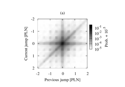
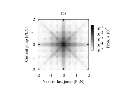
Figure 1: Empirical normalized histograms of different kinds of two price jumps dependences: (a) for the current price jump and the preceding price jump, (b) for the current price jump and the second one before the current price jump or next-to-last jump. The larger logarithm of the joint probability is visualized by more intense grayness. To avoid singularity of the logarithmic scale, all probabilities are increased by small insignificant number $10^{-5}$.

Observed antisymmetric dependence between $r_{n}$ and $r_{n-2}$ can be considered as a generic empirical example of two random variables which are dependent but uncorrelated. Besides a sharp central cross, it contains both a “diagonal” and an “anti-diagonal”. These diagonals and anti-diagonals correspond to the case, where the current price jump and the second one before the current price jump have the same length but might have the same or the opposite signs.

Apparently, Eq. (3) is able to reproduce only the diagonal of the histogram. To reproduce both diagonal and anti-diagonal we ave to extend Eq. (3) into the form

$$h_{2}(r_{n},r_{n-2}) = (1-2\zeta)h(r_{n})h(r_{n-2})$$

$$+ \zeta\ \delta(r_{n}-r_{n-2})h(r_{n-2})$$

$$+ \zeta\ \delta(r_{n}+r_{n-2})h(r_{n-2}),\quad 0\leq\zeta\leq 1,$$

essential for further considerations, where the second and third terms represent diagonal an anti-diagonal, respectively. These terms, together with the first term, make distribution $h_{2}(r_{n},r_{n-2})$ well normalized quantity. To obtain a vanishing correlation between $r_{n}$ and $r_{n-2}$ we assumed weights of the diagonal and anti-diagonal equal and denoted by $\zeta$. Now, we can construct the three-variable pdf of three consecutive price jumps. For simplicity, instead of notation ($r_{n},r_{n-1},r_{n-2}$) we use ($r_{3},r_{2},r_{1}$).

The three-variables pdf, $h(r_{3},r_{2},r_{1})$, should obey the following constrains concerning the marginal distributions:

• Firstly, distribution $h(r_{3},r_{2},r_{1})$ integrated over any two of the three variables should reproduce, for the third variable, a single price jump distribution – the same for all three cases. The analogical constrain for two variables pdf is already satisfied by Eq. (1).

• Secondly, distribution $h(r_{3},r_{2},r_{1})$ integrated over variable $r_{1}$ should reproduce two-variables pdf, $h(r_{3},r_{2})$, in the form of Eq. (1). The same pdf $h(r_{3},r_{2},r_{1})$ integrated over variable $r_{3}$ should also reproduce two-variables pdf, $h(r_{2},r_{1})$, again in the form of Eq. (1).

• However, pdf $h(r_{3},r_{2},r_{1})$ integrated over variable $r_{2}$ should give pdf $h_{2}(r_{3},r_{1})$ in the form of Eq. (LABEL:eq:h2).

Hence, we propose a key formula for $h(r_{3},r_{2},r_{1})$ in the form

$$h(r_{3},r_{2},r_{1}) = (1-2\epsilon)h(r_{3})h(r_{2})h(r_{1})$$ (7)

$$+ \zeta\delta(r_{3}+r_{2})\delta(r_{2}+r_{1})h(r_{1})$$

$$+ (\epsilon-\zeta)\delta(r_{3}+r_{2})h(r_{2})h(r_{1})$$

$$+ (\epsilon-\zeta)\delta(r_{2}+r_{1})h(r_{3})h(r_{1})+$$

$$+ \zeta\delta(r_{3}+r_{1})h(r_{2})h(r_{1}),$$

which satisfies all constrains mentioned above. Obviously, this form is not a unique pdf but it is the simplest one which uses only two parameters ($\epsilon$ and $\zeta$), where additionally each term has clear interpretation.

It is worth to mention that all terms shown on the right-hand side of Eq. (7), except the last one, are present, with slightly modified pre-factors, in the simple product of distributions $h(r_{3}\mid r_{2})$ and $h(r_{2},r_{1})$ defined by Eqs. (1) and (2), respectively. The only new term is the last one, proportional to $\delta(r_{3}+r_{1})h(r_{2})$. This term describes the case, where price jump $r_{1}$ is followed by the second, independent price jump $r_{2}$ and the third price jump $r_{3}=-r_{1}$ which has the same length as jump $r_{1}$ but the opposite sign. The adding of such a term is due to the bid-ask bounce phenomena with delay present herein. We explain what is meant by the name ‘bid-ask bounce with delay’ by using a characteristic scenario given below.

Let us consider a continuous-time double auction market organized by the order book system dacorogna2001 ; ohara1995 ; hasbrouck2006 ; campbell2012 . Let buy and sell orders be sorted according to the corresponding price limit. The gap between buy order with the highest price limit and sell order with the lowest price limit is called the bid-ask spread dacorogna2001 ; ohara1995 ; hasbrouck2006 ; campbell2012 . In our previous paper gubiec2 we analyzed, as a typical example, a series of orders which lead to the bouncing of the price between lower and higher border of the bid-ask spread. To justify the form of Eq. (1), we argued that if the price increases from the lower border of the bid-ask spread to some possibly new value of the higher border, the two cases are possible.

In the first case, an appropriate sell order occurs, with probability $\epsilon$, and the price goes back to the vicinity of the previous price. This results in two consecutive price jumps of approximately the same length but opposite signs. In the second case, if other type of the order arrived, it leads to the elimination of the system memory present in the bid-ask spread. As a result, the subsequent price jump can be considered in this case as independent of the previous jump and appears with probability $1-\epsilon$. These two cases can be formally expressed by the two variable pdf just in the form given by Eq. (1). However, as we argued in the previous section, one-step memory CTRW formalism is not able to properly describe the high frequency stock market dynamics.

Fortunately, from the second case considered above, we are able to extract the subsequent case, leading eventually to the two-step memory. That is, if after the first price jump the executable small volume buy order appeared, the price jump (initiated by this buy order) will also be small or even equals zero. In such a case, the memory of the system is still present in the bid-ask spread, because its lower border still did not move, in fact. Hence, the backward jump to the lower border is still possible with the price jump of approximately the same length as the second to last price jump, but with opposite sign. Analogous dependence can be present for longer series of consecutive jumps but with systematically decreasing order. We emphasize that we do not assume that subsequent orders are independent, so our model even describes a situation where memory is present in the order flow lillo2004

By means of pdf, the term describing such a case (of the two-step memory) can be approximated by the term proportional to $\delta(r_{3}+r_{1})\delta(r_{2})h(r_{1})$. The first Dirac’s delta is responsible for the situation where the current jump $r_{3}$ repeats the second one, $r_{1}$, before the current price jump, but with the opposite sign (i.e. $r_{3}=-r_{1}$). The second Dirac’s delta gives the zero-length mid price jump $r_{2}$. However, to obey all three constrains (a) - (c) on marginal distributions of $h(r_{3},r_{2},r_{1})$, we were forced to use instead of two deltas, the last term based on the product $\delta(r_{3}+r_{1})h(r_{2})h(r_{1})$. Let us remind that single jump distribution $h(r_{2})$ is strongly concentrated at the vicinity of $r_{2}$ equals zero. Taking this term into account with appropriate weight, we thus completed our basic Eq. (7).

In our model the jumps of the process are not independent, as a current jump depends on two preceding jumps. Hence, the conditional pdf of the jump length $r_{3}$, under the condition of previous jumps $r_{2}$ and $r_{1}$, can be obtained from Eq. (7) by dividing of its both sides by $h(r_{2},r_{1})$ given by Eq. (1). This leads to the useful conditional pdf

$$h(r_{3}\mid r_{2},r_{1}) = \left(1-\delta_{r_{2},-r_{1}}\right)$$

$$\times \left(\frac{1-2\epsilon}{1-\epsilon}\ h(r_{3})+\frac{\zeta}{1-\epsilon}\ \delta(r_{3}+r_{1})\right)$$

$$+ \left(1-\delta_{r_{2},-r_{1}}\right)\frac{\epsilon-\zeta}{1-\epsilon}\ \delta(r_{3}+r_{2})$$

$$+ \delta_{r_{2},-r_{1}}\left(\frac{\epsilon-\zeta}{\epsilon}\ h(r_{3})+\frac{\zeta}{\epsilon}\ \delta(r_{3}+r_{2})\right),$$

where the following dependences between Dirac’s delta and Kronecker’s delta were used

$$\left(1-\delta_{x,-y}\right)\delta(x+y) = 0,$$

$$\delta_{x,-y}\delta(x+y) = \delta(x+y).$$

As we precisely defined dependences between consecutive jumps, we can introduce a stochastic process and derive the analytical forms of the most significant quantities such as the propagator and velocity autocorrelation function of the process.

Notably, Eqs. (7) and (LABEL:two:hh) have generic character, which does not limit them to the local dynamics of share price only.

4 Solution

The high-frequency share price time series can be considered as a single realization or trajectory of a jump stochastic process. The trajectory of such a process is a step-way function consisting of waiting times $\tau_{n}$ prior to the sudden jump increment of a price $r_{n}$. Hence, the single trajectory can be defined in time and space by the series of subsequent temporary points

$$\tau_{1},r_{1};\tau_{2},r_{2};\ldots;\tau_{n},r_{n}$$

and the process can be described by the conditional probability density

$$\rho(r_{n},\tau_{n}\,|\,r_{n-1},\tau_{n-1};r_{n-2},\tau_{n-2};\,\dots\,;r_{2},\tau_{2};r_{1},\tau_{1})$$

. This is the probability density of jump increment $r_{n}$ after waiting time $\tau_{n}$, conditioned by the whole history $(\tau_{1},r_{1};\tau_{2},r_{2};\ldots;\tau_{n-1},r_{n-1})$. To construct theoretical model, we have to make the following simplifying assumptions:

• the process is stationary, ergodic and homogeneous in space (price) variable. In the case of financial market, we neglect the influence of the so-called lunch effect, which is the non-stationarity resulting as a daily stable pattern of investors’ activity;

• all waiting times between successive changes of the process, $\tau_{n}$, are i.i.d. random variables with distribution $\psi(\tau_{n})$ having finite average. In case of infinite average the process is non-ergodic bel2005 ; burov2010 ;

• each jump increment $r_{n}$ of the process depends only on two previous jump increments $r_{n-1},r_{n-2}$ in the form given by Eq. (LABEL:two:hh).

The approximations given above can be summarized in the form of a factorized distribution,

$$\rho ( r_{n},\tau_{n}\,|\,r_{n-1},\tau_{n-1};r_{n-2},\tau_{n-2};\,\dots\,;r_{2},\tau_{2};r_{1},\tau_{1})$$ (9)

$$\approx h(r_{n}\,|\,r_{n-1},r_{n-2})\,\psi(\tau_{n}).$$

Equation (9) gives the recipe for the infinitely long trajectory but, as the process is homogeneous and stationary, we can arbitrary choose the origin for the time and space axes. Since we analyze the trajectories starting at some arbitrary time $t=0$ at origin, we have to take into account that the first jump of the process after time $t=0$ depends on the two previous jumps, that we call $r_{0}$ and $r_{-1}$. This can be solved by weighting the trajectories by $h(r_{0},r_{-1})$, where $h$ is given by Eq. (1) even for $n=0$.

Furthermore, we cannot use the same waiting-time distribution for the first jump as for other jumps. This is because jump increment $r_{0}$ might occur at any time before $t=0$. Therefore, we can average over all possible time intervals $\tau^{\prime}$ between the instant of jump increment $r_{0}$ and the time origin $t=0$. Such an averaging was proposed in haus1987 and leads to the distribution

$$\psi_{1}(\tau) = \frac{\int\limits^{\infty}_{0}d\tau^{\prime}\psi(\tau+\tau^{\prime})}{\int\limits^{\infty}_{0}d\tau^{\prime\prime}\int\limits^{\infty}_{0}d\tau^{\prime}\psi(\tau^{\prime}+\tau^{\prime\prime})}$$ (10)

$$\Leftrightarrow \tilde{\psi}_{1}(s)=\frac{1}{\langle\tau\rangle}\frac{1-\tilde{\psi}(s)}{s},$$

where expected (mean) waiting-time is

$$\langle\tau\rangle=\int^{\infty}_{0}\tau\ \psi(\tau)d\tau<\infty$$

. The denominator in the first equation in Eq. (10) is required for the normalization. The only continuous case where $\psi_{1}(\tau)=\psi(\tau)$ is an exponential waiting-time distribution of a Poisson process.

The aim of this section is to derive the conditional probability density, $P\left(X,t\right)$, to find value $X$ of the process at time $t$, at condition that the process initial value was assumed as the origin. Further in the text we call this probability the soft stochastic propagator, in contrast to the sharp one, which we define below. The derivation of the propagator consists of few steps described in the following paragraphs, which extends the corresponding derivation of the canonical CTRW formalism.

The intermediate very useful quantity describing the stochastic process is the sharp, $n$-step propagator

$$Q_{n}\left(X,r_{n},r_{n-1};t\right),n=1,2,\ldots$$

. This propagator is defined as the probability density that the process, which had initially (at $t=0$) the original value ($X=0$), makes its $(n-1)^{th}$ jump by $r_{n-1}$ from $X-r_{n}-r_{n-1}$ to $X-r_{n}$ (at any time) and makes its $n$-th jump by increment $r_{n}$ from $X-r_{n}$ to $X$ exactly at time $t$. The key expression needed for exact solution of the process is given by the recursion relation

$$Q_{n}\left(X,r_{n},r_{n-1};t\right)=\int\limits_{0}^{t}d\tau\,\psi(\tau)\int\limits^{\infty}_{-\infty}dr_{n-2}$$

$$\times \ h(r_{n}\mid r_{n-1},r_{n-2})Q_{n-1}\left(X-r_{n},r_{n-1},r_{n-2};t-\tau\right),$$

$$n = 3,4,$$ (11)

Equation (11) relates two successive sharp propagators by the spatio-tempotral convolution. This equation is valid only for $n\geq 3$ and should be completed by propagators $Q_{1}$ and $Q_{2}$ calculated directly from their definitions (cf. Ref. gubiec2 ).

We define sharp summarized (infinite-many step) propagator $Q\left(X,t\right)$ as follows,

$$Q\left(X,t\right)\stackrel{{\scriptstyle\rm def.}}{{=}}Q_{1}\left(X;t\right)+Q_{2}\left(X;t\right)$$ (12)

$$+ \sum\limits_{n=3}^{\infty}\int\limits^{\infty}_{-\infty}dr_{n}\int\limits^{\infty}_{-\infty}dr_{n-1}Q_{n}\left(X,r_{n},r_{n-1};t\right).$$

Finally, to obtain the soft stochastic propagator, $P\left(X,t\right)$, we use the relation between soft and sharp propagators, which is much easier to consider in the Fourier-Laplace domain

$$\hat{\tilde{P}}(k,s)=\tilde{\Psi}_{1}(s)+\tilde{\Psi}(s)\hat{\tilde{Q}}(k;s),$$ (13)

where $\tilde{O}$ means the Laplace, and $\hat{O}$ Fourier transform of $O$. Sojourn probabilities (in time and Laplace domains) are defined by the corresponding waiting-time distribution

$$\Psi(\tau)=\int\limits_{\tau}^{\infty}\psi(\tau^{\prime})d\tau^{\prime}\Leftrightarrow\tilde{\Psi}(s)=\frac{1-\tilde{\psi}(s)}{s},$$ (14)

wherein $\Psi_{1}(\tau)$ is defined anologously.

To find an explicit form of Eq. (13) the procedure was developed analogous to that for the one-step memory model gubiec2 , although much more tedious (see Appendix B for details). Hence, the Laplace transform of the velocity autocorrelation function (VAF) is given by

$$\tilde{C}(s)=\frac{s^{2}}{2}\left<\tilde{X}^{2}\right>(s)=\frac{\mu_{2}}{2\left\langle\tau\right\rangle}\frac{N(\tilde{\psi},\zeta,\epsilon)}{D(\tilde{\psi},\zeta,\epsilon)},$$ (15)

while numerator, $N(\tilde{\psi},\zeta,\epsilon)$, and denominator, $D(\tilde{\psi},\zeta,\epsilon)$, are defined as follows

$$N(\tilde{\psi},\zeta,\epsilon) = \tilde{\psi}^{3}\zeta\left(\zeta-\epsilon^{2}\right)+\tilde{\psi}^{2}\epsilon\zeta(2(\epsilon-1)\epsilon-\zeta+1)$$

$$+ \tilde{\psi}(1-\epsilon)^{2}\left(2\epsilon^{2}-\zeta\right)-(1-\epsilon)^{2}\epsilon,$$

$$D(\tilde{\psi},\zeta,\epsilon) = \tilde{\psi}^{3}\zeta\left(\zeta-\epsilon^{2}\right)+\tilde{\psi}^{2}\epsilon\zeta(\zeta-2\epsilon+1)$$ (16)

$$+ \tilde{\psi}\zeta(1-\epsilon)^{2}+(1-\epsilon)^{2}\epsilon,$$

where the relation between the stochastic propagator in the Fourier and Laplace domains and the corresponding mean-square displacement was used herein.

As we are interested in a closed form of the VAF in time domain, we find both expressions in Eq. (16) as too complicated to perform the inverse Laplace transformation of Eq. (15), even for simple forms of $\tilde{\psi}(s)$. To keep our model self-consistent (that is, Eq. (LABEL:eq:h2) being an extension of Eq. (3)), we assume

$$\zeta=\epsilon^{2}.$$ (17)

Our estimation of parameter $\zeta$, based on the empirical data, gives this parameter almost equals $\epsilon^{2}$. Hence, relation (17) simplifies both expressions in Eq. (16) eliminating the residual fluctuations of the order of $\zeta-\epsilon^{2}$. Eq. (15) is simplified now into the more useful (formally) quite different forms,

$$\tilde{C}(s) = \frac{\mu_{2}}{2\left\langle\tau\right\rangle}\frac{1-\epsilon\tilde{\psi}(s)-\epsilon^{2}\tilde{\psi}^{2}(s)}{1+\epsilon\tilde{\psi}(s)+\epsilon^{2}\tilde{\psi}^{2}(s)}=\frac{\mu_{2}}{2\left\langle\tau\right\rangle}$$

$$\times \left[1-2\left(\frac{j}{j-1}\ \frac{\epsilon\tilde{\psi}(s)}{\epsilon\tilde{\psi}(s)-j}+\frac{-1}{j-1}\ \frac{\epsilon\tilde{\psi}(s)}{\epsilon\tilde{\psi}(s)-\bar{j}}\right)\right],$$

where root $j=-\frac{1}{2}+i\frac{\sqrt{3}}{2}$ and $\bar{O}$ means a complex conjugate of $O$.

It is worth mentioning that we can obtain power spectra of our process from Eq. (LABEL:rown:regularC) directly by using Wiener-Khinchin theorem kubo . The normalized VAF is given, in time domain, by expression

$$C^{\,n}(t) = \delta(t)-2\epsilon\mathcal{L}^{-1}_{t}\left(\lambda\frac{\tilde{\psi}(s)}{\epsilon\tilde{\psi}(s)-j}+\bar{\lambda}\frac{\tilde{\psi}(s)}{\epsilon\tilde{\psi}(s)-\bar{j}}\right),$$

where ${\cal L}_{t}^{-1}\{\ldots\}$ is an inverse Laplace transform and $\lambda=\frac{j}{j-1}=\frac{1}{2}-i\frac{\sqrt{3}}{6}$. Apparently, the above obtained VAF uses solely the quantities ($\tilde{\psi}(s)$ and parameter $\epsilon$) analogous to that of the one-step memory model gubiec2 .

Moreover, the very regular form of Eq. (LABEL:rown:regularC) and the corresponding result for the model containing the one-step memory backward enables to formulate the conjecture concerning the memory through arbitrary number of steps

$$\tilde{C}(s) = \frac{\mu_{2}}{2\left\langle\tau\right\rangle}\frac{2-\sum_{j=0}^{n}\epsilon^{j}\tilde{\psi}^{j}(s)}{\sum_{j=0}^{n}\epsilon^{j}\tilde{\psi}^{j}(s)}$$

$$= \frac{\mu_{2}}{2\left\langle\tau\right\rangle}\frac{1-2\epsilon\tilde{\psi}(s)+(\epsilon\tilde{\psi}(s))^{n+1}}{1-(\epsilon\tilde{\psi}(s))^{n+1}},\;n=1,2,\ldots,$$

where three terms in denominator of the first equality in Eq. (LABEL:rown:regularC) are treated, herein, as initial terms of a geometric series (accordingly, the numerator is treated). Apparently, for infinite many steps backward, $(n\rightarrow\infty)$, this equation gives the following result,

$$\tilde{C}(s) = \frac{\mu_{2}}{2\left\langle\tau\right\rangle}\frac{2-\sum_{j=0}^{\infty}\epsilon^{j}\tilde{\psi}^{j}(s)}{\sum_{j=0}^{\infty}\epsilon^{j}\tilde{\psi}^{j}(s)}=\frac{\mu_{2}}{2\left\langle\tau\right\rangle}[1-2\epsilon\tilde{\psi}(s)].$$

very useful for our further considerations.

This is a significant issue that the evolution of $\tilde{C}(s)$ is govern in Eqs. (LABEL:rown:regularCmany) and (LABEL:rown:regularCinf) solely by $\tilde{\psi}(s)$. For instance, a multifractality can be directly considered using Eq. (LABEL:rown:regularCinf) if $\psi(t)$ would be conducted in the form of properly suited superstatistics perello2008 ; kasprzak2010 . However, analysis of anomalous diffusion requires, herein, resignation from stationarity. Lack of stationarity, which would appear here, results from the initial situation and not with how the process itself evolves. Therefore, there are no major obstacles to build a non-stationary formalism CTRW containing memory through infinite-many steps. These concepts define research environment in which ergodicity as well as the Bernoulli law of large numbers and hence the Wiener-Khintchine theorem would be broken while central limit theorem should be extened to the Lévy-Khintchine theorem of the canonical representation of stable laws. However, this is already a subject of a separate work.

5 Comparison of the models

In Sec. 2 we discussed selected properties of the one-step memory model and compared them with well known properties of empirical data. Observed disagreement served as inspiration for development of the two- and infinite-step memory model solved in the previous section, where the latter model is based on our conjuction. In the presnt section we study the difference between one-, two-, and infinite-step memory models by using so much significant characteristic as autocorrelation function.

Let us begin with the analysis of the autocorrelation function in the event time. The dependence between any two jumps of the process within the one-step memory model is given by Eq. (4). This dependence results in autocorrelation expressed by Eq. (5). However, in the case of the two-step memory model, the analogous dependence for $k\geq 1$ is a bit more complicated. Fortunately, we obtain autocorrelation functions in the event time solely to $k=4$. These functions are compared in Tab. 1 with the corresponding results for one-step memory model calculated from Eq. (5).

Table 1: Comparison of the two-step memory model with the one-step memory model. Subsequent five values of the event-time autocorrelation function are presented. Apparently, the two-step memory model gives $c(2)=0$ as required by empirical data.

	$c(0)$	$c(1)$	$c(2)$	$c(3)$	$c(4)$
one-step memory	$1$	$-\epsilon$	$\epsilon^{2}$	$-\epsilon^{3}$	$\epsilon^{4}$
two-step memory	$1$	$-\epsilon$	$0$	$\epsilon^{3}$	$-\epsilon^{4}$
empirical data	$1$	$-\epsilon$	$0.0$	$0.0$	$0.0$

It’s worth recalling that empirical lack of the correlation for $k\geq 2$ is considered as a stylized fact in high frequency empirical financial data. As we assumed during the construction of the model, the current version gives $c(2)=0$. Apparently, for $k\geq 3$ both models give autocorrelation functions of the same orders, which for empirical values of $\epsilon$ are negligibly small quantities (see also Sec. 6).

The particularly useful way to visualize the role of the two- and infinite many step memory models is to compare the corresponding velocity autocorrelation functions in a real time. We perform the inverse Laplace transformation in Eqs. (LABEL:two:C) and (LABEL:rown:regularCinf) for the simplest possible exponential waiting-time distribution to highlight the generic difference between the models. We assume

$$\psi(t)=\frac{1}{\left\langle\tau\right\rangle}e^{-t/\left\langle\tau\right\rangle},$$ (22)

where $\left\langle\tau\right\rangle$ is an average of interevent time. Notably, this is solely waiting-time distribution obeying the equality $\psi_{1}(t)=\psi(t)$ for the first step. In the frame of one-step memory model this WTD leads to the normalized VAF in the form (cf. Eq. (23) in gubiec2 )

$$C^{\,n}(t)=\delta(t)-\frac{2\epsilon}{\left\langle\tau\right\rangle}e^{-(1+\epsilon)t/\left\langle\tau\right\rangle}.$$ (23)

Analogously, by substituting Eq. (22) into Eq. (LABEL:two:C) we obtain for the two-step memory model

$$C^{\,n}(t)=\delta(t)-\frac{2\epsilon}{\left\langle\tau\right\rangle}e^{-(1+\epsilon/2)t/\left\langle\tau\right\rangle}\frac{2}{\sqrt{3}}\cos\left(\frac{\sqrt{3}\epsilon}{2}\frac{t}{\left\langle\tau\right\rangle}+\frac{\pi}{6}\right).$$

(24)

It can be easily proved that for $\epsilon\ll 1$ the VAF given by Eq. (24) reduces into Eq. (23). This reduction was expected as within approximation given by Eq. (17) the difference between both models is of the order of $\epsilon^{2}$.

Furthermore, combining the conjecture given by Eq. (LABEL:rown:regularCinf) and the exponential WTD defined by Eq. (22) we easily obtain

$$C^{\,n}(t)=\delta(t)-\frac{2\epsilon}{\left\langle\tau\right\rangle}e^{-\epsilon t/\left\langle\tau\right\rangle}.$$ (25)

The predictions given by Eqs. (23) – (25) for three different values of $\epsilon$ are shown in Fig. 2.

Figure 2: Comparison of velocity autocorrelation functions for one-, two-, and infinite many steps memory models for three different values of parameter $\epsilon=0.05,0.5,0.95$. All curves are based on exponential waiting time distribution given by Eq. (22). For better visualization, the result for $\epsilon=0.05$ was shifted up by $1$, while result for $\epsilon=0.5$ up by $0.5$. For the same reason, all results are deprived of the Dirac’s delta.

As expected, for time $t\gg\left\langle\tau\right\rangle$ the autocorrelations vanish within all three models, while initially autocorrelations begin their evolution from the same value. For the intermediate time, more steps of memory taken into account in the model lead to a strengthen of the VAF. Besides, the increase of parameter $\epsilon$ increases the difference between autrocorrelation functions.

6 Comparison with empirical data

The satisfactory comparison of predicted autocorrelation functions with empirical ones requires gubiec2 :

• the use of sufficiently realistic waiting time distribution $\tilde{\psi}(s)$,

• determination of values of our basic parameter $\epsilon$ from the separate fit to the corresponding empirical histograms, and

• the use of sufficiently effective method of VAF estimation for unevenly spaced elements of time-series (as interevent time intervals have random lengths).

Useful form of waiting-time distribution is a superposition (or weighted sum) of two exponential distributions gubiec2

$$\psi(t) = \frac{w}{\tau_{1}}e^{-t/\tau_{1}}+\frac{1-w}{\tau_{2}}e^{-t/\tau_{2}}$$ (26)

$$\Leftrightarrow \tilde{\psi}(s)=\frac{w}{1+s\tau_{1}}+\frac{1-w}{1+s\tau_{2}},$$

where $0\leq w\leq 1$ is the weight, while $\tau_{1}$ and $\tau_{2}$ are the corresponding (partial) relaxation times. Apparently, this waiting time pdf has sufficiently simple (for the analytical calculations) closed form after the Laplace transformation. Such a form can be easily and satisfactory fitted to the empirical histogram of waiting times (cf. Fig. 4 in ref. gubiec2 ). Besides, this WTD makes the inverse Laplace transformation present in Eq. (LABEL:two:C) an analytically solvable. Finally, we obtain VAF in the useful form

$$C^{n}(t) = \delta(t)-2\epsilon\Big{[}\lambda\left(A_{1}(j)\,e^{-\eta_{1}(j)\,t}+A_{2}(j)\,e^{-\eta_{2}(j)\,t}\right)$$ (27)

$$+ \bar{\lambda}\left(A_{1}(\bar{j})\,e^{-\eta_{1}(\bar{j})\,t}+A_{2}(\bar{j})\,e^{-\eta_{2}(\bar{j})\,t}\right)\Big{]},$$

where

$$\eta_{1,2}(j) = \frac{1}{2j}\left[j(\omega_{1}+\omega_{2})+\epsilon\upsilon\pm\gamma_{1,2}(j)\right],$$

$$\gamma_{1,2}(j) = \sqrt{\left(j(\omega_{1}+\omega_{2})+\epsilon\upsilon\right)^{2}-4j(j+\epsilon)\omega_{1}\omega_{2}},$$

$$A_{1}(j) = \frac{\omega_{1}\omega_{2}-\eta_{1}\upsilon}{j\;(\eta_{2}-\eta_{1})},$$

$$A_{2}(j) = \frac{\omega_{1}\omega_{2}-\eta_{2}\upsilon}{j\;(\eta_{1}-\eta_{2})},$$

$$\omega_{1} = 1/\tau_{1},$$

$$\omega_{2} = 1/\tau_{2},$$

$$\upsilon = w\;\omega_{1}+(1-w)\;\omega_{2}.$$ (28)

Apparently, above given VAF is a nontrivial because it contains the complex prefactors and exponents, which makes its interpretation a more complicated.

Notably, all required parameters $\tau_{1},\tau_{2},w$ and $\epsilon$ are estimated by the separate empirical data without exploiting the empirical VAF. This is a basic result for further considerations. That is, to find parameter $\epsilon$ only set of empirical jump increments are sufficient to have, while for the estimation of remaining parameters only set of empirical waiting times is required and available. We obtained a very promising comparison of our theoretical VAF with its empirical counterpart because this is not a fit as no free parameters were left to make it.

The comparison of our theoretical predictions with the corresponding empirical VAFs is shown in Fig. 3.

Figure 3: Comparison of three normalized autocorrelation functions of price velocity, for instance, for the PGNIG company (from the fuel and energy sector) quoted on the Warsaw Stock Exchange: (i) the empirical one (small black squares), (ii) the theoretical VAF (dotted curve) derived in Ref. gubiec2 for the one-step memory model, (iii) the theoretical VAF (dashed curve) for the two-step memory model, and (iv) the theoretical VAF (solid curve) for the infinite many-step memory model. All models use the waiting time distribution in the form of the weighted sum of two exponential distributions given by Eq. (26). All parameters were fitted to separate data records, so both theoretical curves have no free parameters to fit to the empirical VAF (notably, the required method of determination of the empirical VAF was thoroughly considered in ref. gubiec2 ).

The improved agreement provided by the two- and infinite many step memory models in comparison with the one-step memory model is well seen. However, still small but distinct systematic deviations exist even for the infinite many step memory model (especially for the initial time).

7 Concluding remarks

Hithertoo, only one step backward memory was considered analytically. In the present paper we developed the version of the CTRW formalism which contains memory over two steps backward or dependence between three consecutive jumps of the process. This extended dependence was studied, herein, independently on whether the second order correlations in the system exist or not, which significantly extends the capability of the CTRW formalism. Such an approach suggests that several already existing results could be improved if one step backward memory model used there, would be changed by two step backward memory model.

There are two results which can be considered as an achievement of our work:

• the derivation of the analitycal closed formula for the propagator containing the two-step memory (cf. Eq. (13)), which is a significant extension of the corresponding one from our previous paper (cf. Eq. (17) in Ref. gubiec2 ), without increasing the number of free parameters and functions,

• the conjugtion which enabled derivation of the velocity autocorrelation function containing infinite many step memory, keeping the model still analytically solvable – the solution is even simpler than for those with finite-step memory.

By using propagator (13) we obtained the velocity autocorrelation of the process which was compared with its empirical counterpart (analogously as it was performed in gubiec2 , cf. plot in Fig. 3 in the present paper) strongly improving the agreement.

The approach presented in this work brings a new approach to random walks with memory, because shows that even in the case of a finite diffusion coefficient the dependence through infinitely many steps play an important role in the CTRW formalism, making the VAF much more realistic. However, still presence of a distinct deficit of correlations suggest that perhaps dependence between interevent times should be somehow coupled with a multi-step memory – this is still a challenge.

Appendix A Proof

Below we prove that $c(2)$ is always larger than 0 if only two successive jumps are dependent.

$$c(2) = \frac{1}{\mu_{2}}\int\limits^{\infty}_{-\infty}dr_{n}\int\limits^{\infty}_{-\infty}dr_{n-1}\int\limits^{\infty}_{-\infty}dr_{n-2}\ r_{n}\ r_{n-2}$$ (29)

$$\times h(r_{n}\mid r_{n-1})\ h(r_{n-1},r_{n-2})$$

$$= \frac{1}{\mu_{2}}\int\limits^{\infty}_{-\infty}dr_{n-1}\ h(r_{n-1})\int\limits^{\infty}_{-\infty}dr_{n}\ r_{n}\ h(r_{n}\mid r_{n-1})$$

$$\times \int\limits^{\infty}_{-\infty}dr_{n-2}\ r_{n-2}\ h(r_{n-2}\mid r_{n-1})$$

$$= \frac{1}{\mu_{2}}\int\limits^{\infty}_{-\infty}dr_{n-1}\ h(r_{n-1})$$

$$\times \left(\int\limits^{\infty}_{-\infty}dr_{n}\ r_{n}\ h(r_{n}\mid r_{n-1})\right)^{2}>0.$$

Appendix B Detailed derivation

In this appendix we present detailed procedure of obtaining the propagator of out 2-step memory CTRW model. Let us start with the generalization of the pdf of three consecutive jumps $h(r_{3},r_{2},r_{1})$ given by Eq. (7). Our 2-step memory model is coherent with the 1-step memory model presented in gubiec2 only at the level of two-variable pdfs $h(r_{3},r_{2})$ and $h(r_{2},r_{1})$. Dependance $h_{2}(r_{3},r_{1})$ present in 2-step memory model give by (LABEL:eq:h2) is irreducible to the form obtained within 1-step memory model (3). To obtain such a reducibility we propose to add another, formal parameter $\theta$ in $h(r_{3},r_{2},r_{1})$ form:

$$h(r_{3},r_{2},r_{1}) = (1-2\epsilon+\theta)h(r_{1})h(r_{2})h(r_{3})$$ (30)

$$+ \zeta\delta(r_{3}+r_{2})\delta(r_{2}+r_{1})h(r_{1})$$

$$+ (\zeta-\theta)\delta(r_{3}+r_{1})h(r_{2})h(r_{1})$$

$$+ (\epsilon-\zeta)\delta(r_{2}+r_{1})h(r_{3})h(r_{1})$$

$$+ (\epsilon-\zeta)\delta(r_{3}+r_{2})h(r_{2})h(r_{1}).$$

As a result, for $\theta=0$ Eq. (30) reduces to the form of (7) and for $\theta=\zeta=\epsilon^{2}$ we obtain 1-step memory model.

For simpler notation let us introduce variable:

$$A = \left(\frac{1-2\epsilon+\theta}{1-\epsilon}\right),$$ (31)

$$B = \left(\frac{\zeta-\theta}{1-\epsilon}\right),$$ (32)

$$C = \left(\frac{\epsilon-\zeta}{1-\epsilon}\right),$$ (33)

$$D = \left(\frac{\epsilon-\zeta}{\epsilon}\right),$$ (34)

$$E = \left(\frac{\zeta}{\epsilon}\right).$$ (35)

Conditional pdf $h(r_{3}\mid r_{2},r_{1})$ can be now expressed in the form

$$h(r_{3}\mid r_{2},r_{1}) = \left(1-\delta_{r_{2},-r_{1}}\right)\Big{[}Ah(r_{3})+B\delta(r_{3}+r_{1})$$ (36)

$$+ C\delta(r_{3}+r_{2})\Big{]}+$$

$$+ \delta_{r_{2},-r_{1}}\left[Dh(r_{3})+E\delta(r_{3}+r_{2})\right].$$

The key relation needed for exact solution of the propagator is given by Eq. (11) which we recall below

$$Q_{n}\left(X,r_{n},r_{n-1};t\right) = \int\limits_{0}^{t}dt^{\prime}\psi(t^{\prime})$$

$$\times \int\limits^{\infty}_{-\infty}dr_{n-2}h(r_{n}\mid r_{n-1},r_{n-2})$$

$$\times Q_{n-1}\left(X-r_{n},r_{n-1},r_{n-2};t-t^{\prime}\right),$$

(37)

For the simplicity of notation let us introduce a notation

$$\tilde{Q}_{n}\left(r_{n},r_{n-1}\right) \equiv \int\limits_{0}^{\infty}dt\,\int\limits^{\infty}_{-\infty}dXe^{ikX}\,e^{-st}\,$$ (38)

$$\times Q_{n}\left(X,r_{n},r_{n-1};t\right),$$

where we omit an explicit depandance on varaibles $k$ and $s$.

The key relation (37) in Fourier–Laplace space and with notation defined above, takes the form:

$$\tilde{Q}_{n}\left(r_{n},r_{n-1}\right) = \tilde{\psi}(s)e^{ikr_{n}}\,\int\limits^{\infty}_{-\infty}dr_{n-2}\ h(r_{n}\mid r_{n-1},r_{n-2})$$ (39)

$$\times \tilde{Q}_{n-1}\left(r_{n-1},r_{n-2}\right).$$

As previously, to obtain more intuitive notation we change variables ($r_{n},r_{n-1},r_{n-2}$) to ($r_{3},r_{2},r_{1}$), what gives

$$\frac{1}{\tilde{\psi}(s)}\tilde{Q}_{n}\left(r_{3},r_{2}\right) = e^{ikr_{3}}\,\int\limits^{\infty}_{-\infty}dr_{1}\ h(r_{3}\mid r_{2},r_{1})$$ (40)

$$\times \tilde{Q}_{n-1}\left(r_{2},r_{1}\right).$$

The method which will allow us to solve equation (40), for the given form of $\ h(r_{3}\mid r_{2},r_{1})$ in (36), is to seperate sharp propagator $\tilde{Q}_{n}\left(r_{3},r_{2}\right)$ into two parts: singular and regular given accordingly by :

$$\tilde{Q}^{R}_{n}\left(r_{2},r_{1}\right)=\left(1-\delta_{r_{2},-r_{1}}\right)\tilde{Q}_{n}\left(r_{2},r_{1}\right),$$ (41)

$$\tilde{Q}^{S}_{n}\left(r_{2}\right)=\int\limits^{\infty}_{-\infty}dr_{1}\delta_{r_{2},-r_{1}}\tilde{Q}_{n}\left(r_{2},r_{1}\right).$$ (42)

With the quantities above we can restore $\tilde{Q}_{n}\left(r_{3},r_{2}\right)$, using relation

$$\tilde{Q}_{n}\left(r_{2},r_{1}\right)=\tilde{Q}^{R}_{n}\left(r_{2},r_{1}\right)+\delta(r_{2}+r_{1})\tilde{Q}^{S}_{n}\left(r_{2}\right).$$ (43)

Next, we transform relation (40) substituting $h$ with its exact form (36) and using definitions (41) i (42):

$$e^{-ikr_{3}}\,\frac{\tilde{Q}_{n}\left(r_{3},r_{2}\right)}{\tilde{\psi}(s)}=\tilde{Q}^{S}_{n-1}\left(r_{2}\right)\left[Dh(r_{3})+E\delta(r_{3}+r_{2})\right]$$ (44)

$$+ B\tilde{Q}^{R}_{n-1}\left(r_{2},-r_{3}\right)$$

$$+ \int\limits^{\infty}_{-\infty}dr_{1}\tilde{Q}^{R}_{n-1}\left(r_{2},r_{1}\right)\left[Ah(r_{3})+C\delta(r_{3}+r_{2})\right].$$

The RHS of (44) contains only regular and singular propagators, while on the LHS we still have full propagator $\tilde{Q}_{n}\left(r_{3},r_{2}\right)$. Our aim is to obtain recurance relation between regular and singular propagator.

Let us multiply both sides of the equation above by $\left(1-\delta_{r_{3},-r_{2}}\right)$

$$e^{-ikr_{3}}\,\left(1-\delta_{r_{3},-r_{2}}\right)\frac{\tilde{Q}_{n}\left(r_{3},r_{2}\right)}{\tilde{\psi}(s)}=\tilde{Q}^{S}_{n-1}\left(r_{2}\right)$$ (45)

$$\times \left(1-\delta_{r_{3},-r_{2}}\right)Dh(r_{3})$$

$$+ B\left(1-\delta_{r_{3},-r_{2}}\right)\tilde{Q}^{R}_{n-1}\left(r_{2},-r_{3}\right)+\left(1-\delta_{r_{3},-r_{2}}\right)$$

$$\times Ah(r_{3})\int\limits^{\infty}_{-\infty}dr_{1}\tilde{Q}^{R}_{n-1}\left(r_{2},r_{1}\right),$$

as a result the term containing $\left(1-\delta_{r_{3},-r_{2}}\right)\delta(r_{3}+r_{2})$ disappear. Afterwards, we multiply both sides by $\delta_{r_{3},-r_{2}}$, what leads to

$$e^{-ikr_{3}}\,\frac{1}{\tilde{\psi}(s)}\delta_{r_{3},-r_{2}}\tilde{Q}_{n}\left(r_{3},r_{2}\right)=\tilde{Q}^{S}_{n-1}\left(r_{2}\right)$$

$$\times \left[D\delta_{r_{3},-r_{2}}h(r_{3})+E\delta(r_{3}+r_{2})\right]+B\delta_{r_{3},-r_{2}}\tilde{Q}^{R}_{n-1}\left(r_{2},-r_{3}\right)$$

$$+ \int\limits^{\infty}_{-\infty}dr_{1}\tilde{Q}^{R}_{n-1}\left(r_{2},r_{1}\right)\left[A\delta_{r_{3},-r_{2}}h(r_{3})+C\delta(r_{3}+r_{2})\right].$$

(46)

Now we rewrite relations (45) and (46) in terms of new variables integrating the latter over $r_{2}$

$$e^{-ikr_{3}}\,\frac{\tilde{Q}^{R}_{n}\left(r_{3},r_{2}\right)}{\tilde{\psi}(s)} = Dh(r_{3})\tilde{Q}^{S}_{n-1}\left(r_{2}\right)+B\tilde{Q}^{R}_{n-1}\left(r_{2},-r_{3}\right)$$ (47)

$$+ Ah(r_{3})\int\limits^{\infty}_{-\infty}dr_{1}\tilde{Q}^{R}_{n-1}\left(r_{2},r_{1}\right),$$

$$e^{-ikr_{3}}\,\frac{\tilde{Q}^{S}_{n}\left(r_{3}\right)}{\tilde{\psi}(s)}=E\tilde{Q}^{S}_{n-1}\left(-r_{3}\right)+C\int\limits^{\infty}_{-\infty}dr_{1}\tilde{Q}^{R}_{n-1}\left(-r_{3},r_{1}\right).$$ (48)

As a result we obtained system of two recurrence equations on regular and singular sharp propagators. In order to solve the equations above let us introduce additional functions

$$\textbf{R}_{n}(b,a) = \Re\int\limits^{\infty}_{-\infty}dr_{3}e^{ibkr_{3}}\,\int\limits^{\infty}_{-\infty}dr_{2}e^{iakr_{2}}\,\tilde{Q}^{R}_{n}\left(r_{3},r_{2}\right),$$

$$\textbf{S}_{n}(a) = \Re\int\limits^{\infty}_{-\infty}dre^{iakr}\,\tilde{Q}^{S}_{n}\left(r\right),$$ (50)

$$H(a) = \Re\int\limits^{\infty}_{-\infty}dxe^{iakx}\,h(x),$$ (51)

where operator $\Re$ giver the real part of the complex number. Due to the definition the following properties are satisfied

$$\textbf{R}_{n}(b,a) = \textbf{R}_{n}(-b,a)=\textbf{R}_{n}(b,-a)=\textbf{R}_{n}(-b,-a),$$

$$\textbf{S}_{n}(a) = \textbf{S}_{n}(-a),$$

$$H(a) = H(-a),$$ (52)

or simply the functions are even in all their parameters.

Acting on both sides of Eq. (47) with the operator

$$\Re\int\limits^{\infty}_{-\infty}dr_{3}e^{ibkr_{3}}\,\int\limits^{\infty}_{-\infty}dr_{2}e^{iakr_{2}}\,,$$

on Eq. (48) with operator

$$\Re\int\limits^{\infty}_{-\infty}dr_{3}e^{iakr_{3}}\,$$

and using definitions (LABEL:A:defR) i (50) we obtain

$$\frac{\textbf{R}_{n}(b-1,a)}{\tilde{\psi}(s)} = D\ H(b)\ \textbf{S}_{n-1}(a)+B\ \textbf{R}_{n-1}(a,-b)$$

$$+ A\ H(b)\ \textbf{R}_{n-1}(a,0),$$

$$\frac{\textbf{S}_{n}(b-1)}{\tilde{\psi}(s)} = E\ \textbf{S}_{n-1}(-b)+C\ \textbf{R}_{n-1}(-b,0).$$ (53)

Notably, by basing on (12) in Fourier–Laplace domain, Eq. (43) and definitions (LABEL:A:defR), (50) we obtain

$$\tilde{Q}_{n}\left(k,s\right) = \int\limits^{\infty}_{-\infty}dr_{2}\int\limits^{\infty}_{-\infty}dr_{1}\ \tilde{Q}_{n}\left(k,r_{2},r_{1};s\right)$$ (54)

$$= \int\limits^{\infty}_{-\infty}dr_{2}\int\limits^{\infty}_{-\infty}dr_{1}\ \tilde{Q}^{R}_{n}\left(r_{2},r_{1}\right)+\int\limits^{\infty}_{-\infty}dr_{2}\ \tilde{Q}^{S}_{n}\left(r_{2}\right)$$

$$= \textbf{R}_{n}(0,0)+\textbf{S}_{n}(0).$$

Apparently, the sharp propagator $\tilde{Q}_{n}\left(k,s\right)$ can be expressed by functions $\textbf{R}_{n}$ and $\textbf{S}_{n}$ with all arguments equal to zero. Hence, our aim is to obtain $\textbf{R}_{n}$ and $\textbf{S}_{n}$ with all arguments equal to zero from the recurrance relationns (B) and (53). Let us start with analysis of (B) in four cases, using properties (52):

$$\left(\begin{array}[]{c}a=0\\ b=0\end{array}\right)\,\Rightarrow\frac{\textbf{R}_{n}(1,0)}{\tilde{\psi}(s)} = D\ H(0)\ \textbf{S}_{n-1}(0)+B\ \textbf{R}_{n-1}(0,0)$$

$$+ A\ H(0)\ \textbf{R}_{n-1}(0,0),$$

$$\left(\begin{array}[]{c}a=0\\ b=1\end{array}\right)\,\Rightarrow\frac{\textbf{R}_{n}(0,0)}{\tilde{\psi}(s)} = D\ H(1)\ \textbf{S}_{n-1}(0)+B\ \textbf{R}_{n-1}(0,1)$$

$$+ A\ H(1)\ \textbf{R}_{n-1}(0,0),$$

$$\left(\begin{array}[]{c}a=1\\ b=0\end{array}\right)\,\Rightarrow\frac{\textbf{R}_{n}(1,1)}{\tilde{\psi}(s)} = D\ H(0)\ \textbf{S}_{n-1}(1)+B\ \textbf{R}_{n-1}(1,0)$$

$$+ A\ H(0)\ \textbf{R}_{n-1}(1,0),$$

$$\left(\begin{array}[]{c}a=1\\ b=1\end{array}\right)\,\Rightarrow\frac{\textbf{R}_{n}(0,1)}{\tilde{\psi}(s)} = D\ H(1)\ \textbf{S}_{n-1}(1)+B\ \textbf{R}_{n-1}(1,1)$$ (60)

$$+ A\ H(1)\ \textbf{R}_{n-1}(1,0).$$ (61)

At this place it is resonalble to redefine factors $A,B,C,D,E$ to remove $\tilde{\psi}(s)$ from the relation, what gives

$$A= \tilde{\psi}(s)\left(\frac{1-2\epsilon+\theta}{1-\epsilon}\right),$$

$$B= \tilde{\psi}(s)\left(\frac{\zeta-\theta}{1-\epsilon}\right),$$

$$C= \tilde{\psi}(s)\left(\frac{\epsilon-\zeta}{1-\epsilon}\right),$$

$$D= \tilde{\psi}(s)\left(\frac{\epsilon-\zeta}{\epsilon}\right),$$

$$E= \tilde{\psi}(s)\left(\frac{\zeta}{\epsilon}\right).$$ (62)

After few linear operations on the system of equations (61) we obtain an expression

$$B^{3}\textbf{R}_{n-3}(1,0) = B^{3}D\ H(0)\ \textbf{S}_{n-4}(0)+B^{4}\ \textbf{R}_{n-4}(0,0)$$

$$+ B^{3}A\ H(0)\ \textbf{R}_{n-4}(0,0),$$

$$\textbf{R}_{n}(0,0) = D\ H(1)\ \textbf{S}_{n-1}(0)+B\ \textbf{R}_{n-1}(0,1)$$

$$+ A\ H(1)\ \textbf{R}_{n-1}(0,0),$$

$$B^{2}\textbf{R}_{n-2}(1,1) = B^{2}D\ H(0)\ \textbf{S}_{n-3}(1)+B^{3}\ \textbf{R}_{n-3}(1,0)$$

$$+ B^{2}A\ H(0)\ \textbf{R}_{n-3}(1,0),$$

$$B\textbf{R}_{n-1}(0,1) = BD\ H(1)\ \textbf{S}_{n-2}(1)+B^{2}\ \textbf{R}_{n-2}(1,1)$$

$$+ BA\ H(1)\ \textbf{R}_{n-2}(1,0).$$

Summation of both sides of given above equations gives

$$\textbf{R}_{n}(0,0) = B^{3}D\ H(0)\ \textbf{S}_{n-4}(0)+B^{4}\ \textbf{R}_{n-4}(0,0)$$ (63)

$$+ B^{3}A\ H(0)\ \textbf{R}_{n-4}(0,0)+D\ H(1)\ \textbf{S}_{n-1}(0)$$

$$+ A\ H(1)\ \textbf{R}_{n-1}(0,0)+B^{2}D\ H(0)\ \textbf{S}_{n-3}(1)$$

$$+ B^{2}A\ H(0)\ \textbf{R}_{n-3}(1,0)+BD\ H(1)\ \textbf{S}_{n-2}(1)$$

$$+ BA\ H(1)\ \textbf{R}_{n-2}(1,0).$$

On the RHS of (63) two components signed by $\textbf{R}_{n-3}(1,0)$ and $\textbf{R}_{n-2}(1,0)$ are still present. They can be once more expressed (with help of (61)) by using

$$B^{2}A\ H(0)\textbf{R}_{n-3}(1,0) = AB^{2}D\ H^{2}(0)\ \textbf{S}_{n-4}(0)$$

$$+ AB^{3}\ H(0)\textbf{R}_{n-4}(0,0)$$

$$+ A^{2}B^{2}\ H^{2}(0)\ \textbf{R}_{n-4}(0,0),$$

and

$$BA\ H(1)\textbf{R}_{n-2}(1,0) = ABD\ H(0)\ H(1)\ \textbf{S}_{n-3}(0)$$

$$+ AB^{2}\ H(1)\textbf{R}_{n-3}(0,0)$$

$$+ A^{2}B\ H(0)\ H(1)\ \textbf{R}_{n-3}(0,0).$$

Using relation $H(0)=1$ and substituting above two expressions to Eq. (63) we obtain

$$\textbf{R}_{n}(0,0) = A\ H(1)\ \textbf{R}_{n-1}(0,0)+B^{2}(A+B)^{2}\ \textbf{R}_{n-4}(0,0)$$ (64)

$$+ AB(A+B)\ H(1)\textbf{R}_{n-3}(0,0)+AB^{2}D\ \textbf{S}_{n-4}(0)$$

$$+ ABD\ H(1)\ \textbf{S}_{n-3}(0)+DB^{3}\ \textbf{S}_{n-4}(0)+$$

$$+ D\ H(1)\ \textbf{S}_{n-1}(0)+DB^{2}\ \textbf{S}_{n-3}(1)$$

$$+ DB\ H(1)\ \textbf{S}_{n-2}(1).$$

where function R occurs with argument equal to zero. We still have the function S with the argument equal one. We can express it differently using relation (53) for $b=0$, what gives

$$\textbf{S}_{n}(1) = E\ \textbf{S}_{n-1}(0)+C\ \textbf{R}_{n-1}(0,0).$$ (65)

Hence

$$DB^{2}\textbf{S}_{n-3}(1) = DB^{2}E\ \textbf{S}_{n-4}(0)$$

$$+ DB^{2}C\ \textbf{R}_{n-4}(0,0),$$

$$DB\ H(1)\ \textbf{S}_{n-2}(1) = DBE\ H(1)\ \textbf{S}_{n-3}(0)$$

$$+ DBC\ H(1)\ \textbf{R}_{n-3}(0,0),$$

what substituted to Eq. (64) gives

$$\textbf{R}_{n}(0,0) = A\ H(1)\ \textbf{R}_{n-1}(0,0)+D\ H(1)\ \textbf{S}_{n-1}(0)$$ (66)

$$+ \left[B^{2}(A+B)^{2}+DB^{2}C\right]\textbf{R}_{n-4}(0,0)$$

$$+ \left[AB(A+B)+DBC\right]\ H(1)\textbf{R}_{n-3}(0,0)$$

$$+ DB^{2}\left(A+B+E\right)\textbf{S}_{n-4}(0)$$

$$+ BD\left(A+E\right)H(1)\ \textbf{S}_{n-3}(0),$$

which is the final form with functions R i S with arguments equal zero

To obtain second recurrence relation we rewrite (53) to the form

$$\textbf{S}_{n}(b-1) = E\ \textbf{S}_{n-1}(-b)+C\ \textbf{R}_{n-1}(-b,0).$$

For $b=1$ it gives

$$\textbf{S}_{n}(0) = E\ \textbf{S}_{n-1}(1)+C\ \textbf{R}_{n-1}(1,0),$$

where the term containing $\textbf{S}_{n-1}(1)$ is obtained from (65). It lead to

$$\textbf{S}_{n}(0) = E\ \left(E\ \textbf{S}_{n-2}(0)+C\ \textbf{R}_{n-2}(0,0)\right)+C\ \textbf{R}_{n-1}(1,0).$$

The term containing $\textbf{R}_{n-1}(1,0)$, as previously can be expressed from (61)

$$\textbf{R}_{n-1}(1,0)=D\ \textbf{S}_{n-2}(0)+(B+A)\ \textbf{R}_{n-2}(0,0),$$

what gives the final form of the second recurrence relation

$$\textbf{S}_{n}(0)=(E^{2}+CD)\textbf{S}_{n-2}(0)+C(A+B+E)\ \textbf{R}_{n-2}(0,0).$$ (67)

Now we introduce additional quantities to simplify the notation

$$\textbf{S}_{n} \equiv \textbf{S}_{n}(0),$$ (68)

$$\textbf{R}_{n} \equiv \textbf{R}_{n}(0,0),$$ (69)

S $$= \sum\limits_{n=1}^{\infty}\textbf{S}_{n},$$ (70)

R $$= \sum\limits_{n=1}^{\infty}\textbf{R}_{n}.$$ (71)

Now we perform summation of Eq. (67) from $n=3$ to $\infty$ and a similar summation of Eq. (66) from $n=5$ to $\infty$

$$\left(\textbf{S}-\textbf{S}_{1}-\textbf{S}_{2}\right) = (E^{2}+CD)\textbf{S}$$

$$+ C(A+B+E)\ \textbf{R},$$

$$\left(\textbf{R}-\textbf{R}_{1}-\textbf{R}_{2}-\textbf{R}_{3}-\textbf{R}_{4}\right)$$

$$= A\ H(1)\ \left(\textbf{R}-\textbf{R}_{1}-\textbf{R}_{2}-\textbf{R}_{3}\right)$$

$$+ D\ H(1)\ \left(\textbf{S}-\textbf{S}_{1}-\textbf{S}_{2}-\textbf{S}_{3}\right)$$

$$+ \left[B^{2}(A+B)^{2}+DB^{2}C\right]\textbf{R}$$

$$+ \left[AB(A+B)+DBC\right]\ H(1)\left(\textbf{R}-\textbf{R}_{1}\right)$$

$$+ DB^{2}\left(A+B+E\right)\textbf{S}+BD\left(A+E\right)H(1)\ \left(\textbf{S}-\textbf{S}_{1}\right).$$

By using $\hat{h}=\hat{h}(k)=H(1)$ we find the above given expressions as equivalent to

$$0 = \textbf{S}_{1}+\textbf{S}_{2}+(E^{2}+CD-1)\textbf{S}+C(A+B+E)\textbf{R},$$

$$0 = \textbf{R}\left[-1+A\ \hat{h}+B^{2}(A+B)^{2}+DB^{2}C\right]$$ (72)

$$+ \textbf{R}\left[\left(AB(A+B)+DBC\right)\ \hat{h}\right]$$

$$+ \textbf{S}\left[D\ \hat{h}+DB^{2}\left(A+B+E\right)+BD\left(A+E\right)\hat{h}\right]$$

$$+ \textbf{R}_{1}+\textbf{R}_{2}+\textbf{R}_{3}+\textbf{R}_{4}$$

$$+ A\ \left(-\textbf{R}_{1}-\textbf{R}_{2}-\textbf{R}_{3}\right)\hat{h}$$

$$+ \left[AB(A+B)+DBC\right]\left(-\textbf{R}_{1}\right)\hat{h}$$

$$+ D\ \left(-\textbf{S}_{1}-\textbf{S}_{2}-\textbf{S}_{3}\right)\hat{h}+BD\left(A+E\right)\left(-\textbf{S}_{1}\right)\hat{h}.$$

If we obtain explicitly the forms of $\textbf{R}_{1},\textbf{R}_{2},\textbf{R}_{3},\textbf{R}_{4},\textbf{S}_{1},\textbf{S}_{2},\textbf{S}_{3}$ we are able to reduce the problem of finding the sharp propagator to the problem of solving system of two equations (72) with two variables R i S.

In order to obtain explicit forms of $\textbf{R}_{1},\textbf{R}_{2},\textbf{R}_{3},\textbf{R}_{4},\textbf{S}_{1},\textbf{S}_{2},\textbf{S}_{3}$ we start with explicit form of first four propagators $Q$ calculated directly from the definition and presented in Fourier-Laplace space

$$\frac{\tilde{Q}_{1}\left(k,s\right)}{\tilde{\psi}_{1}(s)} = \int\limits^{\infty}_{-\infty}d\xi_{0}\int\limits^{\infty}_{-\infty}dXe^{ikX}h(X,\xi_{0}),$$

$$\frac{\tilde{Q}_{2}\left(k,s\right)}{\tilde{\psi}_{1}(s)\tilde{\psi}(s)} = \int\limits^{\infty}_{-\infty}dr_{1}\int\limits^{\infty}_{-\infty}dXe^{ikX}e^{ikr_{1}}\ h(X,r_{1}),$$

$$\frac{\tilde{Q}_{3}\left(k,s\right)}{\tilde{\psi}_{1}(s)\tilde{\psi}^{2}(s)} = \int\limits^{\infty}_{-\infty}dr_{1}\int\limits^{\infty}_{-\infty}dr_{2}\int\limits^{\infty}_{-\infty}dXe^{ikX}$$

$$e^{ikr_{1}}e^{ikr_{2}}h(X,r_{2},r_{1}),$$

$$\frac{\tilde{Q}_{4}\left(k,s\right)}{\tilde{\psi}_{1}(s)\tilde{\psi}^{3}(s)} = \int\limits^{\infty}_{-\infty}dr_{1}\int\limits^{\infty}_{-\infty}dr_{2}\int\limits^{\infty}_{-\infty}dr_{3}\int\limits^{\infty}_{-\infty}dXe^{ikX}$$

$$e^{ikr_{1}}e^{ikr_{2}}e^{ikr_{3}}\ h(X\mid r_{3},r_{2})h(r_{3},r_{2},r_{1}).$$

On the basis of Eqs. (68) and (69), (LABEL:A:defR) and (50) as well as (41) and (42) with help of Eq. (38) we obtain

$$\frac{\textbf{S}_{1}}{\tilde{\psi}_{1}(s)} = \epsilon\hat{h},$$

$$\frac{\textbf{R}_{1}}{\tilde{\psi}_{1}(s)} = (1-\epsilon)\hat{h},$$

$$\frac{\textbf{S}_{2}}{\tilde{\psi}_{1}(s)\tilde{\psi}(s)} = \epsilon,$$

$$\frac{\textbf{R}_{2}}{\tilde{\psi}_{1}(s)\tilde{\psi}(s)} = (1-\epsilon)\hat{h}^{2},$$

$$\frac{\textbf{S}_{3}}{\tilde{\psi}_{1}(s)\tilde{\psi}^{2}(s)} = \epsilon\hat{h},$$

$$\frac{\textbf{R}_{3}}{\tilde{\psi}_{1}(s)\tilde{\psi}^{2}(s)} = (1-2\epsilon+\theta)\hat{h}^{3}+(\epsilon-\theta)\hat{h},$$

$$\frac{\textbf{R}_{4}}{\tilde{\psi}_{1}(s)\tilde{\psi}^{3}(s)} = A(1-2\epsilon+\theta)\hat{h}^{4}+B(\zeta-\theta)$$

$$+ \quad\hat{h}^{2}\left[B(1-2\epsilon+\theta)+D\zeta+A(\zeta-\theta)\right]$$

$$+ \quad\hat{h}^{2}(A+B+D)(\epsilon-\zeta).$$

Substituiting the above given equations into (72) and basing on (12), (54), (70) and (71) we get

$$\tilde{Q}(k,s)=\textbf{R}+\textbf{S}=\tilde{\psi}_{1}\frac{N_{1}}{D_{1}}$$ (73)

where

$$N_{1} = -(\epsilon-1)\tilde{\psi}^{3}(\zeta-\theta)$$

$$\times \left[\hat{h}^{2}\left(\epsilon^{2}-\zeta\right)\left(\epsilon^{2}(\zeta-\theta+1)-\zeta\right)-(\epsilon-1)^{2}\epsilon^{2}(\zeta-\theta)\right]$$

$$+ (\epsilon-1)^{3}\epsilon^{2}\tilde{\psi}\left[\left(\hat{h}^{2}-1\right)\epsilon^{2}+\hat{h}^{2}(-\theta)+\epsilon\right]$$

$$- \hat{h}(\epsilon-1)^{3}\tilde{\psi}^{2}\left(\epsilon^{2}(\theta-2\zeta)+\zeta^{2}\right)$$

$$- \hat{h}(\epsilon-1)^{4}\epsilon^{2}-\hat{h}\tilde{\psi}^{4}\left(\epsilon^{2}-\zeta\right)(\zeta-\theta)$$

$$\times \left[\epsilon^{3}+\epsilon^{2}(-\zeta+\theta-1)+\epsilon\zeta(\zeta-\theta-1)+\zeta\right]$$

$$+ \tilde{\psi}^{5}\left(\epsilon^{2}-\zeta\right)^{2}(\zeta-\theta)^{2}$$

and

$$D_{1} = \hat{h}(\epsilon-1)\tilde{\psi}^{5}\left(\epsilon^{2}-\zeta\right)(\zeta-\theta)\left[\epsilon^{2}+\zeta(\zeta-\theta-1)\right]$$

$$+ \hat{h}(\epsilon-1)^{3}\epsilon^{2}\tilde{\psi}(2\epsilon-\theta-1)$$

$$- \hat{h}(\epsilon-1)\tilde{\psi}^{3}$$

$$\times \left[\epsilon^{4}(3\zeta-2\theta)+2\epsilon^{3}\left(\zeta^{2}-2\zeta(\theta+1)+\theta^{2}+\theta\right)\right]$$

$$+ \hat{h}(\epsilon-1)\tilde{\psi}^{3}$$

$$\times \epsilon^{2}\left[(\zeta+1)\theta^{2}-2\zeta(\zeta+2)\theta+\zeta(\zeta(\zeta+4)-2)+\theta\right]$$

$$- \hat{h}(\epsilon-1)\tilde{\psi}^{3}$$

$$\times 2\epsilon\zeta^{2}+\zeta^{2}(\zeta-\theta-1)$$

$$- \tilde{\psi}^{6}\left(\epsilon^{2}-\zeta\right)^{2}(\zeta-\theta)^{2}-(\epsilon-1)^{4}\epsilon^{2}$$

$$+ \epsilon\tilde{\psi}^{4}\left(3\epsilon^{3}-\epsilon^{2}(2\zeta+3)+\epsilon+\zeta^{2}\right)(\zeta-\theta)^{2}$$

$$- (\epsilon-1)^{3}\tilde{\psi}^{2}\left(\epsilon^{3}-2\epsilon^{2}\zeta+\zeta^{2}\right).$$

Notably, RHS of Eq. (73) depends on $s$ only through $\tilde{\psi}=\tilde{\psi}(s)$ and $\tilde{\psi}_{1}=\tilde{\psi}_{1}(s)$, while depends on $k$ only through $\hat{h}=\hat{h}(k)$. We obtained explicit form of the sharp propagator of the process containing two-step memory. Soft propagator can be simply obrained using (13).

Appendix C Variance and velocity autocorrelation function

The results obtained in this appendix are based on explicit form of the process propagator derived in Appendix B for the two-step memory. This propagator was derived in Appendix B from the recursive equation (37) according to a conditional dependence of three consecutive changes in the price given by equation (36). An exact closed form of the propagator $\tilde{Q}\left(k,s\right)$ was given there by Eq. (73). Using Eq. (13), the soft propagator $\tilde{P}(k,s)$ was derived. Next, the Laplace transform of the time-dependent process variance was derived

$$\tilde{m}_{2}(s)=-\left.\frac{\partial^{2}\tilde{P}(k,s)}{\partial k^{2}}\right|_{k=0}=-\frac{\mu_{2}}{s^{2}\left\langle\tau\right\rangle}\frac{N_{2}}{D_{2}}$$ (74)

where, obviously, $\tilde{\psi}=\tilde{\psi}(s)$, while remaining quantities are parameters independent on $s$ and

$$N_{2} = \tilde{\psi}^{3}\left(\zeta-\epsilon^{2}\right)(\zeta-\theta)+(\epsilon-1)^{2}\tilde{\psi}\left(2\epsilon^{2}-\zeta\right)+$$

$$+\epsilon\tilde{\psi}^{2}(2(\epsilon-1)\epsilon-\zeta+1)(\zeta-\theta)-(\epsilon-1)^{2}\epsilon$$

$$D_{2} = \tilde{\psi}^{3}\left(\zeta-\epsilon^{2}\right)(\zeta-\theta)+\epsilon\tilde{\psi}^{2}(-2\epsilon+\zeta+1)(\zeta-\theta)+$$ (75)

$$+(\epsilon-1)^{2}\zeta\tilde{\psi}+(\epsilon-1)^{2}\epsilon$$

Finally, we obtain the Laplace transform of the velocity autocorrelation function of the process where explicit dependence on parameters $\zeta$ and $\theta$ is well seen.

$$C(s,\zeta,\theta)=-\frac{\mu_{2}}{2\left\langle\tau\right\rangle}\frac{N_{2}}{D_{2}}$$ (76)

We remind that for $\zeta=\theta=\epsilon^{2}$ model with two-step memory well reproduces the results of that with one-step memory. Then,

$$C(s,\zeta=\epsilon^{2},\theta=\epsilon^{2}) = \frac{\mu_{2}}{2\left\langle\tau\right\rangle}\frac{1-\epsilon\tilde{\psi}(s)}{1+\epsilon\tilde{\psi}(s)},$$ (77)

which is the result derived already in gubiec2 .

For the autocorrelation function of the process including two-step memory, one just accept the value of the parameter $\theta=0$, what leads to (15)

References

- (1) A.-L. Barabasi. The origin of bursts and heavy tails in human dynamics. Nature, 435(7039):207–211, 2005.
- (2) A. Vazquez, B. Racz, A. Lukacs, and A.-L. Barabasi. Impact of non-poissonian activity patterns on spreading processes. Physical review letters, 98(15):158702, 2007.
- (3) K. Yamasaki, L. Muchnik, S. Havlin, A. Bunde, and H. E. Stanley. Scaling and memory in volatility return intervals in financial markets. Proceedings of the National Academy of Sciences of the United States of America, 102(26):9424–9428, 2005.
- (4) T. Nakamura, K. Kiyono, K. Yoshiuchi, R. Nakahara, Z. R. Struzik, and Y. Yamamoto. Universal scaling law in human behavioral organization. Physical review letters, 99(13):138103, 2007.
- (5) A. Vázquez, J. G. Oliveira, Z. Dezsö, K.-I. Goh, I. Kondor, and A.-L. Barabási. Modeling bursts and heavy tails in human dynamics. Physical Review E, 73(3):036127, 2006.
- (6) J. Perelló, M. Montero, L.i Palatella, I. Simonsen, and J. Masoliver. Entropy of the nordic electricity market: anomalous scaling, spikes, and mean-reversion. Journal of Statistical Mechanics: Theory and Experiment, 2006(11):P11011, 2006.
- (7) E. W. Montroll and G. H. Weiss. Random walks on lattices. II. Journal of Mathematical Physics, 6(2):167–181, 1965.
- (8) H. Scher and E. W. Montroll. Anomalous transit-time dispersion in amorphous solids. Phys. Rev. B, 12(6):2455–2477, Sep 1975.
- (9) G. Pfister and H. Scher. Dispersive (non-gaussian) transient transport in disordered solids. Advances in Physics, 27(5):747–798, 1978.
- (10) E. W. Montroll and M. F. Schlesinger. On the wonderful world of random walks. In J. Lebowitz and E.M. Montroll, editors, Nonequilibrium Phenomena II. From Stochastics to Hydrodynamics, pages 1–121. North-Holland, Amsterdam, 1984.
- (11) G.H. Weiss. A primer of random walkology. In Fractals in Science, pages 119–162. Springer, 1994.
- (12) J.-P. Bouchaud and A. Georges. Anomalous diffusion in disordered media: statistical mechanisms, models and physical applications. Physics reports, 195(4):127–293, 1990.
- (13) W.D. Gill. Drift mobilities in amorphous charge-transfer complexes of trinitrofluorenone and poly-n-vinylcarbazole. Journal of Applied Physics, 43(12):5033–5040, 1972.
- (14) A.J. Campbell, D.D.C. Bradley, and D.G. Lidzey. Space-charge limited conduction with traps in poly (phenylene vinylene) light emitting diodes. Journal of applied physics, 82(12):6326–6342, 1997.
- (15) D. Ben-Avraham and S. Havlin. Diffusion and reactions in fractals and disordered systems. Cambridge University Press, 2000.
- (16) R. Hilfer. On fractional diffusion and its relation with continuous time random walks. In R. Kutner, A. Pȩkalski, and K. Sznajd-Weron, editors, Anomalous Diffusion From Basics to Applications, pages 77–82. Springer, 1999.
- (17) T. Geisel. Levy walks in chaotic systems: Useful formulas and recent applications. In Lévy flights and related topics in physics, pages 151–173. Springer, 1995.
- (18) J. Klafter, G. Zumofen, and M.F. Shlesinger. Lévy description of anomalous diffusion in dynamical systems. In Lévy flights and related topics in physics, pages 196–215. Springer, 1995.
- (19) E.R. Weeks, T.H. Solomon, J.S. Urbach, and H.L. Swinney. Observation of anomalous diffusion and lévy flights. In Lévy Flights and Related Topics in Physics, pages 51–71. Springer, 1995.
- (20) E.R. Weeks and H.L. Swinney. Anomalous diffusion resulting from strongly asymmetric random walks. Physical Review E, 57(5):4915, 1998.
- (21) R. Hempelmann. Hydrogen diffusion in proton conducting oxides and in nanocrystalline metals. In R. Kutner, A. Pȩkalski, and K. Sznajd-Weron, editors, Anomalous Diffusion From Basics to Applications, pages 247–252. Springer, 1999.
- (22) W. Dieterich and P. Maass. Constant dielectric loss in disordered ionic conductors: Theoretical aspects. Solid State Ionics, 180(6):446–450, 2009.
- (23) H. Scher, G. Margolin, R. Metzler, J. Klafter, and B. Berkowitz. The dynamical foundation of fractal stream chemistry: The origin of extremely long retention times. Geophysical Research Letters, 29(5):5–1, 2002.
- (24) J. Nelson. Continuous-time random-walk model of electron transport in nanocrystalline tio_ 2 electrodes. Physical Review B, 59(23):15374, 1999.
- (25) E. Barkai and Y.-Ch. Cheng. Aging continuous time random walks. The Journal of Chemical Physics, 118(14):6167–6178, 2003.
- (26) C. Monthus and J.-P. Bouchaud. Models of traps and glass phenomenology. Journal of Physics A: Mathematical and General, 29(14):3847, 1996.
- (27) G. Margolin and B. Berkowitz. Application of continuous time random walks to transport in porous media. The Journal of Physical Chemistry B, 104(16):3942–3947, 2000.
- (28) A. Helmstetter and D. Sornette. Diffusion of epicenters of earthquake aftershocks, omoris law, and generalized continuous-time random walk models. Physical Review E, 66(6):061104, 2002.
- (29) N. Iyengar, C.K. Peng, R. Morin, A.L. Goldberger, and L.A. Lipsitz. Age-related alterations in the fractal scaling of cardiac interbeat interval dynamics. American Journal of Physiology-Regulatory, Integrative and Comparative Physiology, 271(4):R1078–R1084, 1996.
- (30) M.A. Lomholt, K. Tal, R. Metzler, and J. Klafter. Lévy strategies in intermittent search processes are advantageous. Proceedings of the National Academy of Sciences, 105(32):11055–11059, 2008.
- (31) L. Hufnagel, D. Brockmann, and T. Geisel. The scaling laws of human travel. Nature, 439:462–465, 2006.
- (32) R. Kutner and F. Świtała. Stochastic simulations of time series within Weierstrass - Mandelbrot walks. Quantitative Finance, 3(3):201–211, 2003.
- (33) R. Kutner. Stock market context of the lévy walks with varying velocity. Physica A: Statistical Mechanics and its Applications, 314(1):786–795, 2002.
- (34) E. Scalas. Five years of continuous-time random walks in econophysics. In The Complex Networks of Economic Interactions, pages 3–16. Springer, 2006.
- (35) J. Perelló, J. Masoliver, A. Kasprzak, and R. Kutner. Model for interevent times with long tails and multifractality in human communications: An application to financial trading. Physical Review E, 78(3):036108, 2008.
- (36) A. Kasprzak, R. Kutner, J. Perelló, and J. Masoliver. Higher-order phase transitions on financial markets. The European Physical Journal B, 76(4):513–527, 2010.
- (37) R. Kutner. Hierarchical spatio-temporal coupling in fractional wanderings.(i) continuous-time weierstrass flights. Physica A: Statistical Mechanics and its Applications, 264(1):84–106, 1999.
- (38) R. Kutner and M. Regulski. Hierarchical spatio-temporal coupling in fractional wanderings.(ii). diffusion phase diagram for weierstrass walks. Physica A: Statistical Mechanics and its Applications, 264(1):107–133, 1999.
- (39) R. Metzler and J. Klafter. The random walk’s guide to anomalous diffusion: a fractional dynamics approach. Physics reports, 339(1):1–77, 2000.
- (40) R. Metzler and J. Klafter. The restaurant at the end of the random walk: recent developments in the description of anomalous transport by fractional dynamics. Journal of Physics A: Mathematical and General, 37(31):R161, 2004.
- (41) R. Kutner and J. Masoliver. The Continuous Time Random Walk, still trendy: Fifty-year history, state of art, and outlook. ArXiv e-prints, December 2016.
- (42) J. W. Haus and K. W. Kehr. Diffusion in regular and disordered lattices. Physics Reports, 150(5-6):263 – 406, 1987.
- (43) K.W. Kehr, R. Kutner, and K. Binder. Diffusion in concentrated lattice gases. self-diffusion of noninteracting particles in three-dimensional lattices. Phys. Rev. B, 23(10):4931–4945, 1981.
- (44) T. Springe. Quasielastic neutron scattering for the investigation of diffusive motions in solids and liquids. Springer, 1972.
- (45) R. Kutner and I. Sosnowska. Thermal neutron scattering from a hydrogen-metal system in terms of a general multi-sublattice jump diffusion model i: Theory. Journal of Physics and Chemistry of Solids, 38(7):741–746, 1977.
- (46) M.B. Salamon. Physics of superionic conductors. Physics of Superionic Conductors. Series: Topics in Current Physics, Edited by Myron B. Salamon, 15, 1979.
- (47) R. Kutner. Correlated hopping in honeycomb lattice: tracer diffusion coefficient at arbitrary lattice gas concentration. Journal of Physics C: Solid State Physics, 18(34):6323, 1985.
- (48) M. Montero and J. Masoliver. Nonindependent continuous-time random walks. Physical Review E, 76(6):061115, 2007.
- (49) M. Montero Torralbo. Parrondo-like behavior in continuous-time random walks with memory. Physical Review E, 84:051139, 2011.
- (50) T. Gubiec and R. Kutner. Backward jump continuous-time random walk: An application to market trading. Physical Review E, 82(4):046119, 2010.
- (51) R. Gençay, M. Dacorogna, U.A. Muller, O. Pictet, and R. Olsen. An Introduction to High-Frequency Finance. Elsevier Science, 2001.
- (52) R. S. Tsay. Analysis of financial time series. Wiley Series in Probability and Statistics. Wiley, 2005.
- (53) R. Roll. A simple implicit measure of the effective bid-ask spread in an efficient market. The Journal of Finance, 39(4):1127–1139, 1984.
- (54) M. O’Hara. Market Microstructure Theory. Blackwell Business. Wiley, 1995.
- (55) J. Hasbrouck. Empirical Market Microstructure : The Institutions, Economics, and Econometrics of Securities Trading: The Institutions, Economics, and Econometrics of Securities Trading. Oxford University Press, USA, 2006.
- (56) J.Y. Campbell, A.W. Lo, and A.C. MacKinlay. The Econometrics of Financial Markets. Princeton University Press, 2012.
- (57) F. Lillo and J. D. Farmer. The long memory of the efficient market. Studies in Nonlinear Dynamics & Econometrics, 8(3), 2004.
- (58) G. Bel and E. Barkai. Weak ergodicity breaking in the continuous-time random walk. Physical review letters, 94(24):240602, 2005.
- (59) S. Burov, R. Metzler, and E. Barkai. Aging and nonergodicity beyond the khinchin theorem. Proceedings of the National Academy of Sciences, 107(30):13228–13233, 2010.
- (60) R. Kubo, M. Toda, and N. Hashitsume. Statistical physics: Nonequilibrium statistical mechanics, volume 2. Springer Verlag, 1992.