Multipath Metropolis Simulation of Classical Heisenberg Model

Abstract

Processor cores are becoming less expensive and thus more accessible. To utilize increasing number of available computing elements, good parallel algorithms are necessary. In light of these changes in contemporary computing, multipath Metropolis simulation of classical Heisenberg model is explored. In contrast to the original single–path algorithm, multipath simulation approach is inherently parallel because different random–walk paths are mutually independent. This independence enables easy and efficient harnessing of numerous cores’ computing power in embarrassingly parallel algorithms. Aside form being inherently parallel, multipath simulation approach results in independent and normally distributed simulation output. Normal distribution enables simple and straightforward statistical processing. Thus, multipath simulation results can be easily computed with arbitrary and statistically known precision.

1 Introduction

Contemporary evolution of Monte Carlo (MC) methods in statistical physics is dictated by several important issues. These include (but are not limited to) the development of faster and more efficient algorithms, further improvement of (pseudo)random number generators, reduction of correlation between data, nontrivial statistical analysis as well as construction of more powerful computing machines (see e.g [1, 2, 3] and references therein). A progress in each of uppermentioned fields is welcomed since variety of possible applications may put emphasis on different aspects of simulation and can also initiate the advance in other areas. In the present paper we offer a strategy for circumventing the complications with statistical analysis of correlated data in the case of classical Heisenberg model (CHM). Even though standard methods for dealing with correlated data, such as blocking or jackknife method [4, 5, 6, 7], do exist, it is not hard to imagine the situation in which truly independent simulation results are desirable. For example, the jackknife method is known to fail in some cases [8]. Being used in many different areas of physics as a working model (see [9, 10, 11, 12, 13, 14, 15] and references therein), CHM is perfectley suited for present exposition. Analogus situation holds for the Ising model (IM), which is still atractive for MC simulations, as seen from recent papers [16, 17, 18, 19]. We shall brieflly discuss the simulation of IM on the square lattice from the present point of view in A. Current work is stimulated by recent developments in the hardware industry: over the last couple of decades the price of processing elements has constantly decreased. This trend is, most likely, set to continue for at least another decade more. Hardware manufacturers have turned to multicore systems [20], resulting in computer architectures with more processing elements. Although significantly faster cores are not expected at least in the near future, a rapid increase in the number of computing cores is a reasonable expectation.

When single core computers were dominant, the main concern was efficient utilization of memory and processor cycles. These aspects are still important however, the increasing number of available cores has also led to a new goal: to utilize as many computing cores as possible in efficient and scalable parallel algorithms. Often there is a trade–off, since increasing the number of utilized cores cannot be achieved without a significant increase in the total number of computing cycles. Thus, it is necessary to develop algorithms that utilize available processing elements efficiently. In this context an inherently parallel multipath approach corresponds to contemporary hardware and software trends.

A Metropolis algorithm is originally defined as a single–flip (only one particle moves at a time), single–path (a complete simulation is performed on one, long random–walk path) algorithm [21, p. 1088]. It is an inherently sequential modification of the Monte Carlo scheme, because each configuration depends on the previous one. One value (of some system property) is computed out of the system state after each flip. At the end, all values are averaged. The mean of these values is taken as the simulation result. It is quite an efficient and widely applicable algorithm, though it produces values that are correlated [5] and, because of that, only asymptotically normally distributed [22, 19]. Such distribution complicates statistical analysis. Also, convergence speed is issue in a single–path approach, since it can be prone to entrapment in local minima [23]. To overcome this issue, algorithm improvement that includes more than one random walk path, known as a Metropolis coupled Markov chain Monte Carlo $(MC)^{3}$ is proposed in [24] (see also [25]). A decades old idea of more–than-one–path Metropolis algorithm enhancement is extended in this paper into an embarrassingly parallel and highly scalable multipath simulation approach, appropriate for our highly parallel computing age.

Section 2 gives an overview of the multipath (MP) Metropolis simulation for the CHM. The notions of simulation path (SP) and simulation output (SO), used throughout the text, are defined there. Section 3 contains the discussion on the quality of the output data in the MP simulation. As the output data are uncorrelated by the very construction of the MP simulation, the subsequent statistical analysis is not only greatly simplified, but also made rigorous. Thus, the results presented in Section 3 reveal the most obvious advantage of the MP simulation over standard (i.e. single-path) one. The conection betveen MP and single-path simulation of the CHM is provided in the section 4, with emphasis on the order parameter (spontaneous magnetization). By computing various thermodynamic properties of CHM in MP and single-path simulation, we demonstrate an overall agreement. Finally, the IM on a square lattice is discussed in A, where we test MP simulation against standard single-path approach and the Onsager-Yang solution. Results obtained for models vith continous (CHM) and descrette internal symmetry (IM) give us the reason to bellive that increment in precission/accuracy is possible and that MP simulation could be of use in other cases where standard Markov-chain MC methods apply.

The simulations on large lattices ($L>10$) for CHM were conducted using data storage and computing services of the Supercomputing Center of Galicia (CESGA) [26]. We used the FINISTERRAE [27] (2500 cores, 35 TFLOPS) and SVG [28] (1800 cores) supercomputers running under GNU/Linux operating system. All simulation results presented in this paper were computed using free software C++ library called ”Hypermo” [29], while most of the figures are created with ”Tulipko” [30] interactive visualization tool. More details on ”Tulipko” will be presented elsewhere.

2 Simulation

In this section we define the model, quantities of interest and set up notation to be used throughout the paper. We also specify the way in which simulation is conducted. In order to acquire statistically independent values, to overcome the issue of local minima entrapment and to be able to utilize the now abundant computing cores, the multipath (MP) approach is explored. It produces a normally distributed simulation output, in both ferromagnetic and paramagnetic phase with simulation output values statistically independent by definition. The statistical analysis of data set with such distribution characteristics is straightforward and rigorous, i.e. there is no need for approximations or additional calculations inevitable when working with asymptotic distributions and correlated data. In this approach a Metropolis algorithm is applied on many different paths, all beginning at a randomly chosen state and each path producing only one simulation output (after reaching thermal equilibrium). Beside producing independent output values this approach offers much bigger parallelization potential compared to single–path approach, since computations on each path are mutually independent.

2.1 Classical $O(3)$ Heisenberg model

Classical $O(3)$ Heisenberg model is defined by the Hamiltonian (energy function)

$$H=-\frac{J}{2}\sum_{\bm{n},\bm{\lambda}}\bm{S}_{\bm{n}}\cdot\bm{S}_{\bm{n}+\bm{\lambda}},$$ (1)

where $J$ is constant of coupling between nearest neighbors (nn) spins and summation is taken over all lattice sites $\{\bm{n}\}$, and $\bm{\lambda}$ connects a given site to its nearest neighbors. For $J>0$ the ground state is ferromagnetic, and for $J<0$ antiferromagnetic, but this makes no difference at the classical level. We define the energy scale by fixing the exchange integral $J=1$. The set $\{\bm{S}_{\bm{n}}\}$ represent spin vectors on a periodic simple cubic lattice with $N=L^{3}$ sites, whose position is defined by the totality of $\{\bm{n}\}$. We employ the standard spherical parametrization

$$\bm{S}_{\bm{n}}=[\sin\theta_{\bm{n}}\cos\varphi_{\bm{n}},\sin\theta_{\bm{n}}\sin\varphi_{\bm{n}},\cos\theta_{\bm{n}}]^{\mathsf{T}}$$ (2)

for unit vectors.

2.2 Definitions and notation

Metropolis single spin–flip algorithm is used to simulate a 3-dimensional classical Heisenberg on a simple cubic lattice. All simulations discussed in this paper are conducted on a particular lattice size at a particular temperature. Each simulation consists of a certain number of simulation paths (simulation path, SP). Each SP produces output which consists of four values $\{M_{i}^{x},M_{i}^{y},M_{i}^{z},H_{i}\}$, where index $i=1,2,\dots,\mathcal{N}$ labels the simulation paths. The first three components in each output define the instantenous total spin per lattice site, $\bm{M}=(1/L^{3})\sum_{\bm{n}}\bm{S}_{\bm{n}}$, while the fourth one is the instanteous energy per lattice site.

Outputs of all the $\mathcal{N}$ SPs, together, form a simulation output (SO). SO that meets desired precision and accuracy is called representative. Additional statistical and physical computations on representative SO are necessary in order to obtain particular physical values, these are referred to as simulation results (simulation result, SR).

Each SP starts from a randomly chosen state which corresponds to infinitely high temperature state [31]. Initial state is selected by randomizing the states of all lattice sites i.e. by randomly choosing values of both angles at all lattice sites. After the initial randomization, Metropolis algorithm is applied to a number of sites in an attempt to reach some thermal equilibrium state of the lattice. Execution of Metropolis algorithm on $L^{3}$ randomly chosen lattice sites is referred to as one lattice sweep (LS) [3]. In every SP a number of LSs is conducted. The SP output is computed out of the last lattice state i.e. from the final state of the Markov chain (state after the last LS). The MC averages are then computed as

$$\langle A\rangle=\frac{1}{\mathcal{N}}\sum_{i=1}^{\mathcal{N}}A_{i}$$ (3)

Specifically, the magnetization and the internal energy are defined as SO average values

$$\langle\bm{M}\rangle=\frac{1}{{\mathcal{N}}}\sum_{i=1}^{\mathcal{N}}\bm{M}_{i},\hskip 28.45274pt\langle H\rangle=\frac{1}{\mathcal{N}}\sum_{i=1}^{\mathcal{N}}H_{i}.$$ (4)

We also make use of

$$\langle M^{k}\rangle=\langle|\bm{M}|^{k}\rangle=\frac{1}{{\mathcal{N}}}\sum_{i=1}^{\mathcal{N}}({M}_{i})^{k},\hskip 28.45274ptM_{i}=\sqrt{(M^{x}_{i})^{2}+(M^{y}_{i})^{2}+(M^{x}_{i})^{2}}$$ (5)

for $k=1,2,4$. In particular, $\langle M\rangle$ plays the role of order parameter on finite lattices. We shall further consider susceptibility and heat capacity

$$\chi(T)=\frac{L^{3}}{T}\left[\langle|\bm{M}|^{2}\rangle-\langle|\bm{M}|\rangle^{2}\right],\hskip 28.45274ptC_{V}(T)=\frac{L^{3}}{T^{2}}\left[\langle H^{2}\rangle-\langle H\rangle^{2}\right].$$ (6)

All thermodynamic quantities, obtained both in standard single-path and multipath method, will be calculated per lattice site. Finally, the transition temperature for infinite lattice is obtained from the intersection of fourth order cumulants [3]

$$U_{L}=1-\frac{1}{3}\frac{\langle M^{4}\rangle}{\langle M^{2}\rangle^{2}}$$ (7)

for different linear finite lattice dimensions $L$.

3 Simulation output

As already stated, the MP simulation is designed so that it produces statistically independent output. To confirm SO independence, output components distribution is carefully examined in ferro and para phase.

Figure 1: (Color online) Energy distribution histogram — ordered and disordered phase ($L=10$)

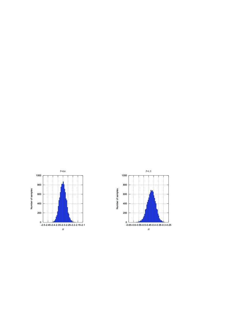
Figure 1 shows SO energy distribution in both the ordered phase ($T=0.6$) and the disordered phase ($T=1.5$). In both phases energy is normally distributed, confirming SO independence. SO energy values $\langle H\rangle$ accumulate around internal energy per site (median). We observed that energy is a little more dispersed in the para phase (the right histogram is a little lower and wider).

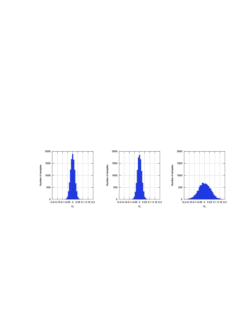
Likewise, Figure 2 shows that the distributions of all three total spin components in the disordered phase are normally distributed, accumulating around zero. The $M_{z}$ component is significantly more dispersed than the other two components since temperature $T=1.5$ is not far from the ordered phase. $M_{z}$ dispersion decreases as the lattice goes deeper into the disordered phase.

Figure 2: (Color online) Total spin components distribution — histogram — disordered phase ($L=10$, $T=1.5$)

Normal Q–Q plot (sometimes also called normal probability plot) is a graphical method for assessing whether or not a data set is approximately normally distributed. It is a special case of Q–Q plot, in which normal distribution is plotted on the $x$–axis. In normal Q–Q plot a data set is plotted in such a way that the points should form the straight line if normal distribution is a good fit for the set.

Figure 3: (Color online) Total spin components distribution — Q–Q plot — disordered phase. Inverse standard normal distribution, i.e. normal theoretical points, are plotted on $x$-axis. ($L=10$, $T=1.5$)

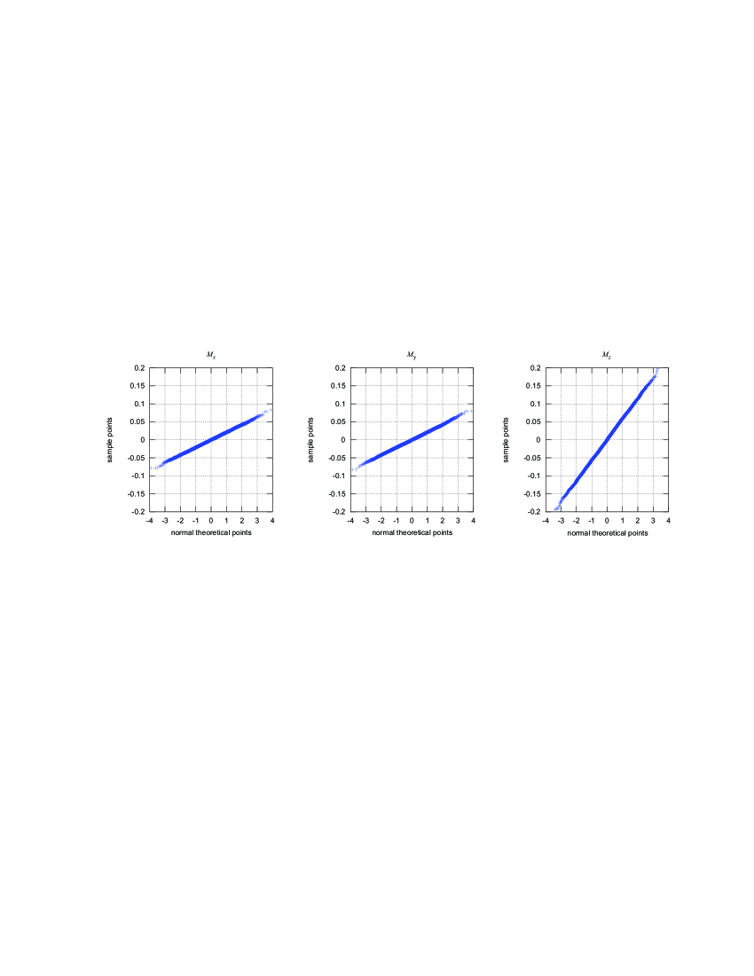
Figure 3 shows the distributions of all three total spin components, similar to Figure 2, but this time as normal Q–Q plots. It is obvious that points can be neatly fitted to the line.

For quantitatively measuring the goodness of the fit, the second norm of the fit residuals can be used [32, p. 210]:

$$norm(R,2)=\sqrt{\sum_{i=1}^{N}R_{i}^{2}};\qquad R_{i}=X_{i}-f(i)$$ (8)

where $R$ represents fit residuals set, $X$ is fitted data set and $f$ is fitting function. Unfortunately, norm depends on the absolute values of the residuals and as such cannot be used for comparison between different fits. Instead, for comparison between samples with different means, correlation coefficient can be used. It will be referred to as distribution coefficient and is defined as:

$$r=1-\frac{norm(R,2)^{2}}{(N-1)\sigma^{2}};\qquad 0\leq r\leq 1$$ (9)

where $R$ represents fit residuals set, $N$ is number of fitted points (number of elements in the $X$ set) and $\sigma$ is standard deviation of the fitted data set $X$. Closer the value of $r$ is to one, closer the sample distribution is to the perfect normal distribution. Distribution coefficients for magnetization components $M_{x}$, $M_{y}$ and $M_{z}$ denoted as $r_{M_{x}}$, $r_{M_{y}}$ and $r_{M_{z}}$ respectively for number of temperatures are shown in Table 1. The table shows that distribution coefficients in ordered phase are very close to 1, confirming that total spin components’ distributions are very close to the normal one.

$T$	$r_{H}$	$r_{M_{x}}$	$r_{M_{y}}$	$r_{M_{z}}$	$r_{|M_{z}|}$
0.6	0.9994	0.9998	0.9998	—	0.9990
0.8	0.9988	0.9990	0.9987	—	0.9983
1.0	0.9994	0.9999	0.9998	—	0.9951
1.2	0.9979	0.9983	0.9989	0.9856	—
1.4	0.9988	0.9998	0.9998	0.9998	—
1.6	0.9995	0.9999	0.9999	0.9999	—

Table 1: $L=10$. Distribution coefficient $r$ is number from $0$ to $1$ which describes how close are points plotted on Q–Q plot to the straight line i.e. how close is data sample distribution to the normal distribution.

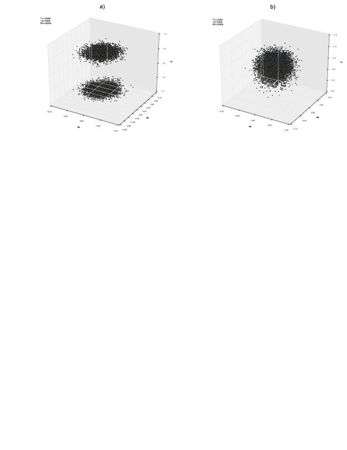
Total spin components distributions in the ferromagnetic phase are shown in Figure 4. It is seen that $M_{x}$ and $M_{y}$ are normally distributed, as in the paramagnetic phase. Note that $M_{x}$ and $M_{y}$ group around $\langle M_{x}\rangle=\langle M_{y}\rangle=0$, in both the ferro and para phases. $M_{z}$ values form two independent normal distributions (see, e.g., [33] for the case of the Ising model), which reflects the symmetry $S_{\bm{n}}^{z}\rightarrow-S_{\bm{n}}^{z}$ of the Hamiltonian (1). As a consequence of this symmetry, magnetization (defined in (4)) is null vector. This illustrates the well known fact that there is no spontaneous symmetry breaking on finite lattices.

Figure 4: (Color online) Total spin components distribution — histogram — ordered phase ($L=10$, $T=0.6$). d) and e) shows enlarged picks from c).

Figure 5: (Color online) Total spin components distribution — Q–Q plot — ordered phase. Inverse standard normal distribution, i.e. normal theoretical points, are plotted on $x$-axis. ($L=10$, $T=0.6$)

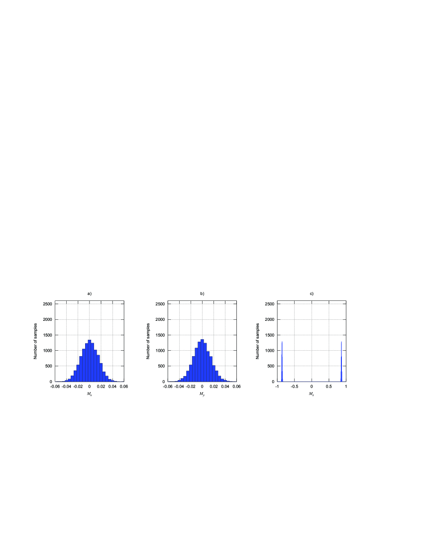
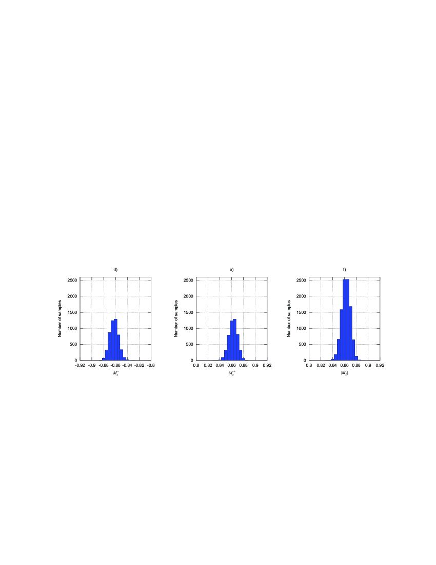
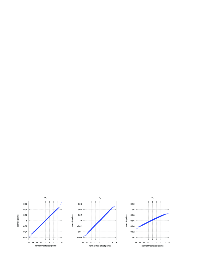
Figure 5 shows distributions of $M_{x}$, $M_{y}$ and $|M_{z}|$ total spin components in an ordered phase on Q–Q plot. As on histograms (Figure 4), normal distribution of components is observed but $|M_{z}|$ component dispersion is smaller compared to dispersions of the other two components. In the disordered phase there is just one accumulation point for $M_{z}$ values similarly to $M_{x}$ and $M_{y}$. Thus, distribution coefficient for the $M_{z}$ component is $r_{M_{z}}$ (Table 1). In the ordered phase $M_{z}$ values accumulate symmetrically around two points: $M_{z}^{-}$ and $M_{z}^{+}$, forming two normal distributions. In order to determine the distribution coefficient, these two sets of points are combined in one absolute values set. Thus, the distribution coefficient for $M_{z}$ in this phase is $r_{|M_{z}|}$. Trying to correlate the distribution of signed $M_{z}$ values to the single normal one in the ordered phase is meaningless. Similarly, there is no correlation between the absolute $M_{z}$ values and normal distribution in the disordered phase. Thus, the $r_{M_{z}}$ values in the ordered phase are marked with ’—’ as are the $r_{|M_{z}|}$ values in the disordered phase. Values from the table confirm an almost perfect fit to the straight line and hence to the normal distribution for energy as well as for all three total spin components in both the ordered and the disordered phase.

Figure 6: (Color online) Total spin distribution in 3D ($L=10,T=0.6$). Red–blue color boundary indicates vectors with $\langle{M}\rangle$ intensity. Green line indicates the direction of $z$-axes. The midpoint of green line denotes the origin in the internal space of total spin vectors.

Figure 7: (Color online) Total spin distribution in 3D ($L=10$, $T=1.5$). Red–blue color boundary emphasizes sphere with $\langle{M}\rangle$ radius. Green line indicates the direction of $z$-axes. The midpoint of green line denotes the origin in the internal space of total spin vectors.

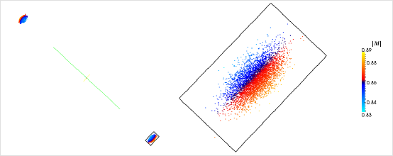
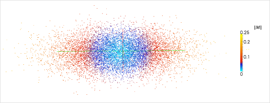
Figure 6 shows the total spin vectors intensity and orientation in space at a low temperature ($T=0.6,L=10$). The initial point of all vectors is located at the origin and the colored dots represent terminal points of the vectors. Vectors group around the $z$-axis in two bundles, as already discussed (Figure 4). In contrast, in the disordered phase spins are distributed in the subspace of internal space around the origin, as shown on Figure 7 ($T=1.5,L=10$). The radius of the blue sphere on Figure 7 represent a residual value of $\langle M\rangle$ (see also Figure 11 bellow). Note that the ellipsoidal character of the total spin vector distribution in the disordered phase (Figure 7) is merely an artifact of the parametrization (2). Calculations show that the distribution (Figure 7) reduces to spherical form with temperature increase.

To get a better insight into the angle distribution of total spin vectors, we plot $\bm{M}/|\bm{M}|$ for various temperatures in Figure 8. This figure also gives complete information of total spin vectors $\bm{M}$ since the color represents the magnitude of $\bm{M}$.

Figure 8: (Color online) Distribution of normalized total spin ($\bm{M}/|\bm{M}|$) for different temperatures. Colors represent magnitude of the vector $\bm{M}$. (L=10)

The order parameter $\langle{M}\rangle$ for the lattice with 10 lattice sites in each dimension ($L=10$), on different temperatures is plotted against the number of LSs (Figure 9a). Each simulation is conducted on $1000$ simulation paths. The resulting figure exhibits two distinct parts. In the first part magnetization rises rapidly with an increase in the number of LSs. This part of the figure represents states that are walked trough while most of the lattices are still far from the thermal equilibrium state, also called ’the warm-up phase’. The second part is based on representative or close–to–representative states, thus $\langle{M}\rangle$ in this part fluctuates mildly around the true value.

Figure 9: (Color online) $L=10$; a) The order parameter $\langle{M}\rangle$ against number of LSs for $\mathcal{N}=1000$ SPs for different temperatures — number of LSs required to reach equilibrium decreases with increase of temperature; b) coefficient of variation (10) of $\langle{M}\rangle$ against number of LSs. When not shown, the error bars are smaller than symbols.

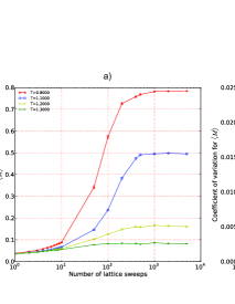
In our experiments the number of LSs is approximately doubled for each new simulation, so that details on the figure are much easier to observe if plotted on a semi–log plot, especially for the small LS values (In contrast, a linear plot provides a better idea of thermalization duration and cost). With the rise in temperature, $\langle{M}\rangle$ is diminishing, as expected. The number of LSs necessary for almost all lattices to reach equilibrium is also reducing. For $T=0.8$ thermalization takes $5\times 10^{3}$ LSs but for $T=1.3$ only $500$ LSs is required.

Data set variability can be expressed in a number of different ways. Usually variance or standard deviation are used. Both of these values are related to the data set mean and as such cannot be used for comparison of data sets with different mean values. When such comparison is needed, coefficient of variation (cv) can be used. Care should be taken because cv is meaningful only for data sets with positive means. Coefficient of variation of a data set mean is given by:

$$cv_{\bar{X}}=\frac{\sigma_{\bar{X}}}{\bar{X}}=\frac{\sigma_{X}}{\sqrt{N}\bar{X}}$$ (10)

where $X$ represents any data set, $N$ number of elements in the set $X$, $\bar{X}$ the data set mean, $\sigma_{X}$ standard deviation of the set $X$ and $\sigma_{\bar{X}}$ stands for standard deviation of the set mean $\bar{X}$.

Coefficients of variation of the $\langle{M}\rangle$ against number of LSs are plotted on the Figure 9b), also for $1000$ simulation paths. The figure shows that as simulation goes deeper in the disordered phase SO dispersion is bigger thus an increase in the coefficient of variation can be observed. In order to get the same precision at higher temperatures it is necessary to compute more simulation paths.

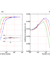
The order parameter $\langle{M}\rangle$ and the coefficient of variation of the order parameter mean for the $L=10$ lattice in the ordered phase ($T=1.0$) for a different number of SPs are plotted against the number of LSs are shown on Figure 10 a) and Figure 10b). When most of the path–chains reach equilibrium (around $500$ LSs) the coefficient of variation becomes quite small (just a couple of percents) even if only a couple of paths are used. That is, most of the intensities $\bm{M}_{i}$ entering (4) get very close to their mean value $\langle{M}\rangle$, thus producing quite accurate and precise outputs. If just an approximate result is needed, a simulation with just a few paths can be used to quickly and cheaply produce a reasonable estimate. A similar plot, this time for the disordered phase, is shown in Figure 10 c) and Figure 10 d). In the disordered phase there is a much bigger dispersion due to significant thermal disturbances. Thus, the coefficient of variation is larger compared to the ordered phase, even after thermalization equilibrium has been reached (around $100$ LSs for $L=10$ and $T=1.5$).

$\langle{M}\rangle$ and the coefficient of variation of the $\langle{M}\rangle$ are shown against number of LSs conducted in ordered phase ($T=1.0$) for different lattice sizes (Figure 11). Each simulation is performed on 1000 SPs. Larger lattices generate more accurate (Figure 11a) and more precise (Figure 11b) output but require more LSs to reach a representative state (i.e. to reach thermal equilibrium). Similar plots, just for the disordered phase ($T=1.5$), are also given in Figure 11. The inset on Figure 11a) shows a close-up of the region in which the value of order parameter converges. With an increase of lattice size accuracy improvements can be noticed, as $\langle{M}\rangle$ is approaching zero (Figure 11c). Since thermal disturbance is significant in the disordered phase there is no increase in precision (Figure 11d).

Figure 10: (Color online) a) The order parameter $\langle{M}\rangle$ and b) the coefficient of variation (10) (ordered phase, $L=10,T=1.0$) together with c) the order parameter and d) the coefficient of variation (disordered phase, $L=10,T=1.5$) against number of LSs for different number of SPs ($\mathcal{N}$). When not shown, the error bars are smaller than symbols.

Figure 11: (Color online) a) The order parameter $\langle{M}\rangle$ and b) coefficient of variation (10) (ordered phase, $L=10,T=1.0$) together with c) the order parameter and d) the coefficient of variation (disordered phase, $L=10,T=1.5$) against the number of LSs for $L=10,15,20$. $\mathcal{N}=10^{3}$ both in the ordered and disordered phase. When not shown, the error bars are smaller than symbols. The inset on first graph shows a close-up of the convergence region.

The number of lattice sweeps needed for a lattice to reach it’s representative state (also called burn-in or warm–up phase) is unknown. It depends on many parameters and can vary substantially. Insufficient number of lattice sweeps causes inaccurate simulation results. To overcome this problem for each temperature half of the simulation paths are computed from the random initial state where other half started from the ordered state (see Figure 12) These two sets are averaged using (3) but results from each half separately. When both halves produce the same result (see Figure 13) we can be reasonably certain that it is an accurate value.

Figure 12: (Color online) Distribution of total spin at $T=1$, for $5\times 10^{3}$ lattice sweeps and $\mathcal{N}=10^{4}$ simulation paths. Every path started a) from random spin configuration and b) from ordered configuration.

Figure 13: (Color online) a) Magnetization and b) coefficient of variation for $L=10$, $T=1$, calculated starting from both ordered and disordered states, as a function of number of lattice sweeps for $\mathcal{N}=10000$. Red dot represents single-path result. When not shown, the error bars are smaller than the symbols.

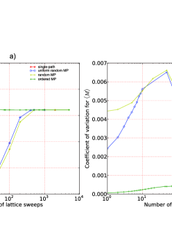
At this point we make connection with standard (single-path) simulation and show that the states generated by each path are truly representative ones. To do so, we examine the value of the ordered parameter for $L=10$ and $T=1$ (see Figure 13) and show that single-path and MP results converge to the same value. The single path result obtained from $10^{4}$ measurements is represented by red star on Figure 13 and the error, estimated by the blocking method, is less than the size of symbol. The ordered state is used as a starting point in the single-path simulation. On the other hand, MP value is obtained from $10^{4}$ simulation paths. Three sets of data correspond to three different initial configurations: ordered state (green symbols), the initial state with all angles taking arbitrary values (yellow symbols) and the uniform state where unit vectors are uniformly distributed on the sphere (blue symbols). It is seen that, within the error which is $\sim 10^{-4}$, all of them converge to the same value of the order parameter. Thus, we conclude that the final states on each path are indeed representative ones. Moreover, the Figure 10a) shows that the value of $\langle M\rangle$, obtained with just several hundreds of paths comes very close to the convergence point. All of this should not come as a surprise, since each path represents one Markov chain whose trajectory through the phase space is governed by the Metropolis algorithm.

4 Thermodynamics of classical Heisenberg model

Further justification of the MP approach comes from the study of thermodynamic properties of CHM over wide temperature range. We examine spontaneous magnetization (the ordered parameter), energy, susceptibility and specific heat per lattice site and compare results from MP and single-path simulation. All simulations were conducted for the system with $N=10^{3}$ lattice sites and periodic boundary condition, both in single and multipath approach. In single–path approach we used $2\times 10^{6}$ lattice sweeps to achieve thermal equilibrium in whole temperature range, and afterwards one out of every five lattice sweeps was used to calculate the averages of physical quantities [34]. At every temperature $5\times 10^{5}$ measurements were averaged. To make sure that reliable results are generated by multipath simulation, it is prepared in two different setups. In the first one, refered to as random initial state simulation in the text, at every lattice site both angles $\theta$ and $\varphi$ are taken to be arbitrary. In the second one, denoted as ordered initial state simulation spins are taken to points along z-axis, with no restriction on second spherical angle $\varphi$. The MP simulation is conducted with $\mathcal{N}=10^{4}$ SPs. The results are shown on Figures 14 and 15 and they reveal that the differences in the thermodynamical characteristic obtained by single–path and multipath approach are negligible.

Figure 14: (Color online) a) Magnetization and b) energy as functions of temperature for $L=10$ in the single–path and multipath approach.

Figure 15: (Color online) a)Magnetic susceptibility and b) heat capacity as functions of temperature for $L=10$ in the single–path and multipath approach.

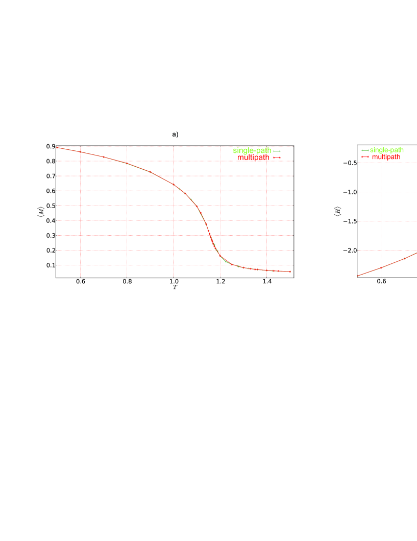
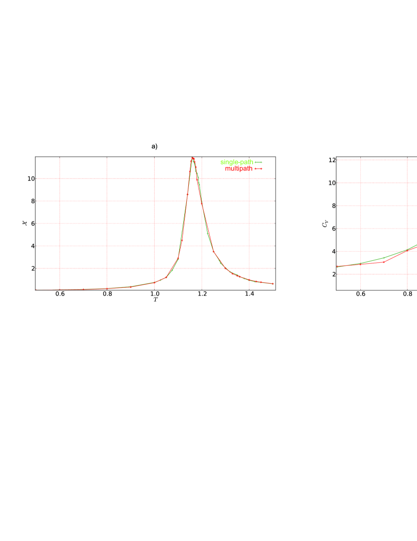
The analysis from previous section indicates that the increase in the number of lattice sweeps, simulation paths and the lattice sites, leading to the enhancement in precision and accuracy, should reduce this difference even further. We have to bear in mind, however, that multipath simulations naturally split into three temperature domains in which different numbers of lattice sweeps/simulation paths are needed. In low temperature region for simulation convergence more lattice sweeps is needed since all paths start from some random state of the lattice. (Simulation speed can be optimized if ordered state is taken to be ”starting point” of all paths.) On the other hand, high temperature region requires more simulation paths. In the critical region we take sufficiently large number of lattice sweeps and results due to overlapping of the distinct output distributions [33].

Figure 16: (Color online) Determination of the critical temperature: the ratio of Binder cumulants $U_{30}$ and $U_{20}$ calculated for $T=1.44$ and $T=1.45$ (blue symbols)

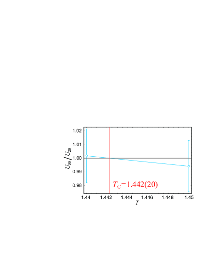
As another illustration of the multipath approach, we calculate the critical temperature of $O(3)$ CHM. It is estimated from the condition $U_{L}(T_{\mathrm{C}})/U_{L^{\prime}}(T_{\mathrm{C}})=1$ for $L=30$ and $L^{\prime}=20$. Simulations for each lattice size on $T=1.44$ and $T=1.45$ were conducted using $10^{6}$ SPs and 200 lattice sweeps. The results are shown on Figure 16 and the final result is $T_{\mathrm{C}}=1.442(20)$ i.e. $\beta_{\mathrm{C}}=0.693(9)$. The standard estimates for the inverse critical temperature of CHM, are $\beta_{\mathrm{C}}=0.69300(10)$ [35], $\beta_{\mathrm{C}}=0.693035(37)$ [36] and $\beta_{\mathrm{C}}=0.693002(12)$ [37] (se also [38]). Thus, the current MP simulation, with only 200 lattice sweeps, reaches three-digit precision for $\beta_{\mathrm{C}}$. One should note that the values quoted from papers [35, 36, 37] are obtained using cluster algorithms, larger lattices (up to $L=48$) and with significantly more laattice sweeps (For example, the authors of [36] used $10^{6}$ measurments after $1-7\times 10^{4}$ single-cluster updatings). Nevertheless, the results from Section 3 indicate that the more precise value for $T_{\mathrm{C}}$ (i.e. $\beta_{\mathrm{C}}$) is expected when MP simulation is conducted on larger lattices with more lattice sweeps and simulation paths. Of course, the shortening of each single chain (i.e. shortening of sequentially dependent algorithm parts) compared to an increase in total number of LSs (i.e. increase in total number of processor cycles utilized) is obviously a trade-off and depends on the problem in question. The detailed study of critical behaviour of CHM, employing MP technique, is a work in progress.

5 Conclusions

The Metropolis algorithm applied to multiple random–walk paths becomes an embarrassingly parallel algorithm in which plenty of cores can be utilized easily. Multipath approach produces normally distributed simulation output with an easily computable error margin. Also, this approach is local minima entrapment resilient by definition. Multipath approach is based on a slightly modified Metropolis algorithm as it generates just one representayive state after a number of thermalization sweeps, conducted for warm–up. Therefore Markov chain on each simulation path is significantly shorter than the chain in the equivalent single–path simulation. Usually path lengths differ by a couple of orders of magnitude, offering tremendous parallelization speedups.

The present paper is mainly devoted to investigation of the order parameter (spontaneous magnetization). While results from first half of Section 3 demonstrate the quality of output data, remaining ones from 3 and those from Section 4 reveal, beside inherent normal distribution of output results, two more important aspects of MP simulation of CHM. First, each path generates representative states, since MC average with just several hundreds of simulation paths (or less) yields reasonable estimate of the order parameter. Second, MC averages of the order parameter calculated in MP and single-path simulation coincide (within errorr bars) over wide temperature range. On the other hand, the quantitative description of the critical region (high-precision determination of the critical temperature and critical indices), recquires a similar analysis for higher-order moments.

Appendix A 2D Ising model

Figure 17: (Color online) Results of MP simulations for Ising model on square lattice. The parameters of simulations are given in the text.

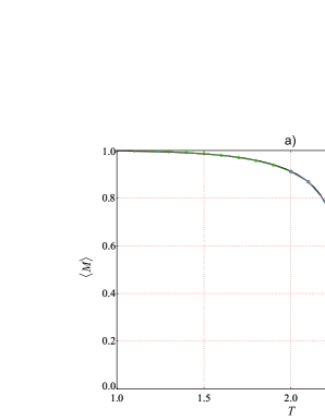
To test the applicability of MP simulation on anisotropic systems, we examine it on 2D Ising model. The exact solution of this model is known, so MP simulations can be checked against Onsager–Jang result. As in the case of CHM, we shall focus on the order parameter.

The setup of the MP simulation is the same as in the case of $O(3)$ CHM. This means that each path start from random state of the lattice and contributes to MC averages with its final state. The Figure 17 displays MP results for spontaneous magnetization on latices $20\times 20,40\times 40,50\times 50$ and $60\times 60$. Each simulation is conducted with $3\times 10^{4}$ lattice sweeps and $10^{4}$ SPs. Specificaly, Figure 17a) shows the order parameter as a function of temperature for several lattices, together with Onzager-Yang solution [39]. As expected, simulations on larger lattices produce more accurate values of spontaneous magnetization. Further, the convergence of MC average of the ordeder parameter and corresponding coefitient of variation against number of lattice sweeps are shown in para–phase [$T=3$, Figures  17b) and c)] and in ferro–phase [$T=1$, Figure 17d) and e)]. All graphs from Figure  17 ilustrate that order parameters of models with continous (CHM) and discrete (IM) symmetry behave similarly in MP simulation. Thus, the entire analysis and all conclusions from Sections 3 and 4 apply almost without any change to IM. Finally, we determine the critical temperature of IM on square lattice by method of Binder cumulants. By using lattices $50\times 50$ and $60\times 60$ for $T=2.264$ and $T=2.268$ in MP simulation with $3\times 10^{4}$ lattice sweeps and $5\times 10^{4}$ SPs, we obtain $T_{\mathrm{C}}=2.269(10)$. This value agrees with exact solution in three decimal places As in the case of CHM, a simulation on larger lattice and with more lattice sweeps and SPs is nedeed for more precise value of the critical temperature.

References

- [1] K. Binder, E. Luijten, Monte carlo tests of renormalization-group predictions for critical phenomena in ising models, Physics Reports 344 (2001) 179–253.
- [2] D. M. Ceperley, Microscopic simulations in physics, Reviews of Modern Physics 71 (1999) S438.
- [3] D. P. Landau, K. Binder, A guide to Monte Carlo simulations in statistical physics, Cambridge university press, 2005.
- [4] H. Flyvbjerg, H. G. Petersen, Error estimates on averages of correlated data, The Journal of Chemical Physics 91 (1989) 461.
- [5] A. M. Ferrenberg, D. P. Landau, K. Binder, Statistical and Systematic Errors in Monte Carlo Sampling, Journal of statistical physics 63 (5-6) (1991) 867–882.
- [6] C. Whitmer, Over-relaxation methods for Monte Carlo simulations of quadratic and multiquadratic actions, Physical Review D 29 (2) (1984) 306.
- [7] J. J. Morales, M. J. Nuevo, L. F. Rull, Statistical error methods in computer simulations, Journal of Computational Physics 89 (2) (1990) 432–438.
- [8] B. Efron, Bootstrap Methods: Another Look at the Jackknife, The Annals of Statisticss 7 (1979) 1.
- [9] J. Zinn-Justin, Quantum Field Theory and Critical Phenomena, Clarendon Press Oxford, 2002.
- [10] A. P. Young, B. S. Shastry, Theory of the spin dynamics of paramagnetic EuO and EuS, Journal of Physics C: Solid State Physics 15 (21) (1982) 4547.
- [11] R. M. Nowotny, K. Binder, Classical Heisenberg antiferromagnets with nearest and next-nearest neighbor interactions on the face-centered cubic lattice: a model for EuTe?, Zeitschrift für Physik B Condensed Matter 77 (2) (1989) 287–301.
- [12] H. E. Stanley, T. A. Kaplan, High - Temperature Expansions the Classical Heisenberg model, Physical Review Letters 16 (22) (1966) 981–983.
- [13] W. Bialek, A. Cavagna, I. Giardina, T. Mora, E. Silvestri, M. Viale, A. M. Walczak, Statistical mechanics for natural flocks of birds, Proceedings of the National Academy of Sciences 109 (13) (2012) 4786–4791.
- [14] S. Naji, A. Benyoussef, A. El Kenz, H. Ez-Zahraouy, M. Loulidi, Monte Carlo Study of phase transitions and magnetic properties of LaMnO3: Heisenberg model, Physica A: Statistical Mechanics and its Applications 391 (15) (2012) 3885–3894.
-
[15]
S. Tsai, A. Bunker, D. P. Landau,
Dynamic
critical behavior of the classical anisotropic {BCC} heisenberg
antiferromagnet, Computer Physics Communications 147 (1–2) (2002) 97 –
100.
doi:10.1016/S0010-4655(02)00224-2.
URL http://www.sciencedirect.com/science/article/pii/S0010465502002242 - [16] T. Preis, P. Virnau, W. Paul, J. J. Schneider, GPU accelerated Monte Carlo simulation of the 2D and 3D Ising model, Journal of Computational Physics 228 (12) (2009) 4468–4477.
- [17] B. Block, P. Virnau, T. Preis, Multi-GPU accelerated multi-spin Monte Carlo simulations of the 2D Ising model, Computer Physics Communications 181 (9) (2010) 1549–1556.
- [18] M. Weigel, Performance potential for simulating spin models on GPU, Journal of Computational Physics 231 (8) (2012) 3064–3082.
- [19] Y. Lin, F. Wang, X. Zheng, H. Gao, L. Zhang, Monte Carlo simulation of the Ising model on FPGA, Journal of Computational Physics 237 (2012) 224–234.
- [20] D. Geer, Chip makers turn to multicore processors, Computer 38 (5) (2005) 11–13. doi:10.1109/MC.2005.160.
- [21] N. Metropolis, A. W. Rosenbluth, M. N. Rosenbluth, A. H. Teller, E. Teller, Equation of State Calculations by Fast Computing Machines, The journal of chemical physics 21 (1953) 1087–1092.
- [22] H. Müller-Krumbhaar, K. Binder, Dynamic properties of the Monte Carlo method in statistical mechanics, Journal of Statistical Physics 8 (1) (1973) 1–24.
- [23] G. Altekar, S. Dwarkadas, J. P. Huelsenbeck, F. Ronquist, Parallel Metropolis coupled Markov chain Monte Carlo for Bayesian phylogenetic inference, Bioinformatics 20 (3) (2004) 407–415.
- [24] C. J. Geyer, Markov Chain Monte Carlo Maximum Likelihood, in: Computing Science and Statistics: Proceedings of the 23rd Symposium on the Interface, Interface Foundation of North America, 1991, pp. 156–163.
- [25] G. C. J., Practical Markov Chain Monte Carlo, Statistical Science 7 (4).
[26]
The Centre of Supercomputing of Galicia (CESGA)
[online] (2013).
URL http://www.cesga.es -
[27]
FINISTERRAE
computing system installed in CESGA [online] (2013).
URL https://www.cesga.es/en/infraestructuras/computacion/finisterrae -
[28]
SVG computing
system installed in CESGA [online] (2013).
URL https://www.cesga.es/en/infraestructuras/computacion/svg -
[29]
P. S. Rakić, The
Hypermo library [online] (2013).
URL http://bitbucket.org/predrag-rakic/hypermo/ -
[30]
T. Petrić, The tulip
visualization tool [online] (2013).
URL http://bitbucket.org/iTrustedYOu/tulip - [31] K. Binder, D. W. Heermann, Monte Carlo simulation in statistical physics: an introduction, Springer, 2010.
- [32] J. S. Hansen, GNU Octave: Beginner’s Guide, Packt Pub Limited, 2011.
- [33] K. Binder, Finite Size Scaling Analysis of Ising Model Block Distribution Functions, Zeitschrift für Physik B Condensed Matter 43 (2) (1981) 119–140.
- [34] C. C. Price, N. B. Perkins, Critical properties of the kitaev-heisenberg model, Physical review letters 109 (2012) 187201.
- [35] C. Holm, W. Janke, Critical exponents of the classical three-dimensional Heisenberg model: A single cluster Monte Carlo simulation, Physical Review B 48 (2) (1993) 936–950.
- [36] K. Chen, A. M. Ferrenberg, D. P. Landau, Static critical behavior of three-dimensional classical Heisenberg models: A high-resolution Monte Carlo study, Physical Review B 48 (5) (1993) 3249.
- [37] H. Ballesteros, L. Fernandez, V. Martin-Mayor, A. Munoz Sudupe, Finite size effects on measures of critical exponents in models, Physics Letters B 387 (1) (1996) 125–131.
- [38] P. Butera, M. Comi, N-vector spin models on the simple-cubic and the body-centered-cubic lattices: A study of the critical behavior of the susceptibility and of the correlation length by high-temperature series extended to order , Physical Review B 56 (13) (1997) 8212.
- [39] T. D. Schultz, D. C. Mattis, E. H. Lieb, Two-dimensional Ising Model as a Soluble Problem of Many Fermions, Reviews of Modern Physics 36 (3) (1964) 856.