Thermodynamic Properties of the Anisotropic Frustrated Spin-chain Compound Linarite PbCuSO₄(OH)₂

Abstract

We present a comprehensive macroscopic thermodynamic study of the quasi-one-dimensional (1D) $s=\tfrac{1}{2}$ frustrated spin-chain system linarite. Susceptibility, magnetization, specific heat, magnetocaloric effect, magnetostriction, and thermal-expansion measurements were performed to characterize the magnetic phase diagram. In particular, for magnetic fields along the $b$ axis five different magnetic regions have been detected, some of them exhibiting short-range-order effects. The experimental magnetic entropy and magnetization are compared to a theoretical modelling of these quantities using DMRG and TMRG approaches. Within the framework of a purely 1D isotropic model Hamiltonian, only a qualitative agreement between theory and the experimental data can be achieved. Instead, it is demonstrated that a significant symmetric anisotropic exchange of about 10 % is necessary to account for the basic experimental observations, including the 3D saturation field, and which in turn might stabilize a triatic (three-magnon) multipolar phase.

I Introduction

Within the last four decades modern research on magnetic materials has focussed on studying low-dimensional (quantum) spin systems Lake et al. (2005); Sebastian et al. (2006). From such investigations, these compounds have been found to possess exotic physical ground-state properties such as resonating valence bond Anderson (1987), quantum spin liquid Han et al. (2012), and spin Peierls ground states Hase et al. (1993).

Nearly one-dimensional (1D) coupled quantum magnets can be realized, for instance, in chain-like arrangements of spins of $s=\tfrac{1}{2}$ Cu²⁺ or V⁴⁺ cations, that are typically surrounded by oxygen anions. In general, the basic building blocks of a Cu-oxide spin-chain system are CuO₄ plaquettes which are connected to each other along one crystallographic direction, viz., one dimension. Here, we focus on this type of copper oxides, where one needs to distinguish between two different classes of materials. In one class of compounds the linkage along the chain occurs at the corners of the plaquettes, thus forming the so-called corner-sharing chain. This geometrical configuration leads to a linear Cu-O-Cu bond between neighboring Cu ions. Then, the oxygen 2$p$ orbitals hybridize with the copper 3$d$ orbitals with a straight bond angle of 180^∘, hence the Goodenough-Kanamori-Anderson rules predict a strong antiferromagnetic (AFM) exchange interaction along the chain between all nearest-neighbor (NN) Cu ions resulting essentially in an unfrustrated system. These systems can be described to the first approximation by the now reasonably well understood simple AFM Heisenberg models extensively studied theoretically for more than eighty years.

In contrast, a second class of compounds contains edge-sharing CuO₄ units. In this situation the bond angle between the nearest Cu-ion neighbors (NN), Cu-O-Cu, is close to 90^∘, which leads in most cases to a ferromagnetic coupling (FM) along this bond. The AFM superexchange contribution is very weak for such a geometry according to the Goodenough-Kanamori-Anderson rules, since it vanishes exactly in the case of a 90^∘ Cu-O-Cu bond angle. Under such circumstances the dominant FM $J_{1}$ stems mainly from the relatively direct large FM interaction $K_{pd}\approx 900$ K between holes on neighboring oxygen and copper sites Mizuno et al. (1999); Lorenz et al. (2009); Kuzian et al. (2012) and not from the Hunds coupling between the mentioned two oxygen orbitals as frequently believed. The latter contributes about 20 % to the value of $J_{1}$, only. In comparison, the next-nearest-neighbor (NNN) Cu-O-O-Cu exchange paths contain $\sigma$ bonds of oxygen $2p$ orbitals resulting in an AFM coupling which always causes frustration effects, irrespective of the sign of the NN coupling and in particular it is almost independent of $K_{pd}$, in sharp contrast to $J_{1}$ which exhibits a very sensitive linear dependence on $K_{pd}$ Málek and Drechsler (2013). Comparable to the first case, in this second class of compounds the NN and NNN interactions are often similar in magnitude leading to strong frustration which offers a large variety of possible ground states. The scientific history of this class and the related quantum models are much younger (tracing back to the last decade) than that of the simpler well-investigated AFM Heisenberg $s=\tfrac{1}{2}$ chain.

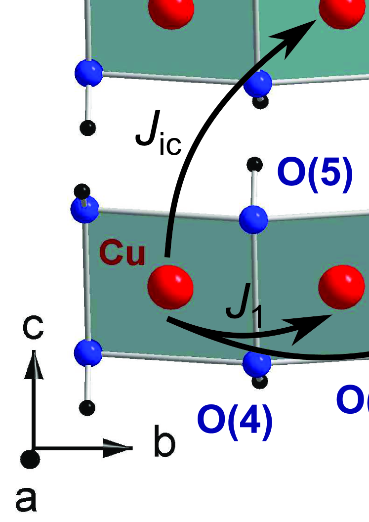
Figure 1: (Color online) Upper part: The crystallographic structure of PbCuSO₄(OH)₂ consisting of buckled neutral Cu(OH)₂ chains propagating along the crystallographic $b$ direction surrounded by Pb²⁺ cations and SO${}_{4}^{2-}$ anions. Lower panel, left: The main exchange paths $J_{1}$ and $J_{2}$ (notation in the general anisotropic case for the two intrachain exchange paths shown would be $\Delta_{1}J_{1}$ and $\Delta_{2}J_{2}$, see Eq. 1 and the text below) in the basal $bc$ plane as well as the dominant skew interchain coupling $J_{\text{ic}}$. The photographic picture shows one of our mineral specimens from the Grand Reef Mine in Graham County, Arizona.

Various Cu-oxide materials have been discovered which represent excellent experimental realizations of such quasi-1D quantum magnets (Q1DQM), e.g., LiCuVO₄ Enderle et al. (2005), LiCu₂O₂ Gippius et al. (2004); Park et al. (2007), Li₂ZrCuO₄ Drechsler et al. (2007), and LiCuSbO₄ Dutton et al. (2012). The basic model to describe the interplay of the NN and NNN exchange for the magnetic properties is the so-called 1D isotropic $J_{1}$-$J_{2}$ or zig-zag chain (ladder) model, which corresponds to the Hamiltonian

$$\begin{split}\hat{H}&=J_{1}\sum_{l}{\bf S}_{l}\cdot{\bf S}_{l+1}+J_{2}\sum_{l}{\bf S}_{l}\cdot{\bf S}_{l+2}+\\ &+\sum_{l}\left(D_{1}-1\right)J_{1}{S}^{z}_{l}{S}^{z}_{l+1}+\left(D_{2}-1\right)J_{2}{S}^{z}_{l}{S}^{z}_{l+2}+\\ &-h\sum_{l}S_{l}^{z}\end{split}$$ (1)

Here, $J_{1}<0$ is the FM NN-interaction, $J_{2}>0$ is the AFM NNN exchange, and $h=g\mu_{B}H$ represents the external magnetic field along the easy ($z$) direction. The symmetric exchange anisotropy rem (a) terms with the anisotropy parameters $D_{1,2}$ to be discussed in Sec. V are given in the second line of Eq. 1. Depending on the frustration ratio $\alpha=-J_{2}/J_{1}$ and within the limits of a classical approach with isotropic exchange, theory predicts various ground states for this class of materials: For an $\alpha$ value $0<\alpha<\tfrac{1}{4}$ a FM ground state should occur, a value between $-\tfrac{1}{4}<\alpha<0$ should result in a collinear AFM Néel ground state, while for all other values a non-collinear spin-spiral ground state is predicted Hamada et al. (1988); Tonegawa and Harada (1989).

If we also consider weak interchain interaction, anisotropic couplings and quantum fluctuations, which may actually strongly affect the 3D magnetic ordering, theory predicts even more exotic ground states Furukawa et al. (2010). Moreover, by applying an external magnetic field a rich variety of exotic field-induced phases may occur in these materials Hikihara et al. (2008); Sudan et al. (2009); Zhitomirsky and Tsunetsugu (2010). The recent discovery of multiferroicity in LiCu₂O₂ Park et al. (2007); Seki et al. (2008) and LiCuVO₄ Naito et al. (2007); Schrettle et al. (2008); Mourigal et al. (2011), as predicted by theory Katsura et al. (2005); Sergienko and Dagotto (2006); Mostovoy (2006); Xiang and Whangbo (2007) for spin-chain systems with a helical ground state, has opened up another playground in this research area. Unfortunately, the Li⁺ ions tend to interchange with the Cu²⁺ ions in the aforementioned materials, therefore, the microscopic source for multiferroicity has not yet been established Moskvin and Drechsler (2008); Moskvin et al. (2009).

Consequently, in order to experimentally investigate these different phenomena and ground states, a material is required which ideally exists in single crystal form without positional disorder, exhibits anisotropic exchange, and possesses a saturation field that is within experimental reach. In a recent investigation we have shown Wolter et al. (2012) that the natural mineral linarite, PbCuSO₄(OH)₂, satisfies all of these requirements, thus offering unique possibilities to study a variety of the above-mentioned physical topics.

Linarite crystallizes in a monoclinic lattice (space-group symmetry $P2_{1}/m$; $a=9.682$ Å, $b=5.646$ Å, $c=4.683$ Å, $\beta$ = $102.65^{\circ}$ Schofield et al. (2009)). In linarite the chains are formed by Cu(OH)₄ units connected along the $b$ direction in a buckled, edge-sharing geometry. In a previous study Wolter et al. (2012) the $b$ direction was found to be the easy axis of the system. Consequently, the Cu²⁺ ions ($3d^{9}$ configuration) form an $s=\tfrac{1}{2}$ quasi-1D spin chain along the $b$ direction (illustrated in Fig. 1), since the distance between two neighboring Cu ions along the $b$ direction is much smaller than along the other crystallographic directions. The surrounding oxygen orbitals mediate the main exchange between the spins residing on the Cu ions along the chain. As explained above, the $J_{1}$ is FM and the largest coupling in the whole system. Due to the competition between that FM NN and the AFM NNN exchange linarite has been established as a magnetically frustrated system. Each oxygen atom binds a hydrogen atom, whereas in between the chains one SO₄ tetrahedron and one lead atom complete the elemental unit cell. The latter act as spacers between the chains and are responsible for its quasi-1D nature.

A recent detailed study of the paramagnetic regime of linarite revealed the coupling constants to be $J_{1}\approx-100$ K and $J_{2}\approx 36$ K Wolter et al. (2012). In effect, a frustration ratio $\alpha=-J_{2}/J_{1}\approx 0.36$ is found, which is much closer to the 1D critical point ($\alpha=0.25$) as compared to the values reported in earlier studies Baran et al. (2006); Yasui et al. (2011). Because of a finite interchain coupling the system undergoes a transition into a long-range magnetically ordered state below $T\approx 2.8$ K. The magnetic ground state was found to consist of an elliptical helical structure with an incommensurate propagation vector ${\bf k}=(0,\,0.186,\,0.5)$ Willenberg et al. (2012).

Here, we present an extensive study of the physical properties of linarite in zero and applied magnetic fields. We will show that relatively weak magnetic fields of a few Tesla have a significant influence on the physical properties of linarite and on the low-temperature specific heat, in particular. This behavior can qualitatively be explained within the framework of the model of a NN-NNN frustrated spin chain, if other terms such as exchange anisotropy are included in the Hamiltonian. The paper is organized as follows: First, we present an extensive study of the low-temperature thermodynamics in zero and applied field of single-crystalline linarite. From the data we establish the magnetic phase diagram for the three crystallographic directions. Finally, we discuss our data, in particular in context of numerical modelling approaches based on one-dimensional spin models and extensions to these.

II Experimental

II.1 Samples and diffraction

The single crystals of PbCuSO₄(OH)₂ used in this study are natural minerals from different sources. In Tab. 1, a summary is presented on the use of the different crystals for the set of experimental methods employed in this work. All crystals show well-defined facets and the principal axes $b$ and $c$ can be identified easily. With these also the normal to the $bc$ plane, $a_{\perp}$, is determined (see Ref. Wolter et al. (2012) for this particular choice of crystal direction). The crystal quality of our samples have been checked by Laue X-ray diffraction. For all sets of single crystals no magnetic impurity phases were observed within experimental resolution, as evidenced by the absence of a low-temperature Curie tail in the magnetic susceptibility. For all measurements the samples were oriented along the crystallographic directions $a_{\perp}$, $b$, and $c$ with a possible misalignment of less than $5^{\circ}$.

II.2 Susceptibility and magnetization

In the ⁴He temperature range, the DC susceptibility was measured by using a commercial vibrating sample magnetometer (VSM). Magnetization measurements for magnetic fields along $a_{\perp}$, $b$, and $c$ at fixed temperatures between 1.8 and 2.8 K have been performed using a Physical Properties Measurement System (PPMS) with a VSM inset. Magnetization data were collected while sweeping the magnetic field using sweep rates of about 300 mT/min for both increasing and decreasing fields. Note that due to hysteresis around the phase transitions observed at 1.8 K, the sweep rate was significantly varied in these field regions in order to check for sweep-rate dependent effects. Using quasi-static conditions, the observed small hysteresis in the $M$($\mu_{0}H$) curves became negligible, as it is shown below.

For DC susceptibility and magnetization measurements down to temperatures of 250 mK an in-house-built cantilever magnetometer was used, which works like a Faraday-force magnetometer. This set-up was used to perform magnetization measurements in applied magnetic fields up to 12 T for $H\parallel b$ with a sweep rate of 4 mT/min.

Table 1: List of linarite crystals used for the experiments presented in this work and former studies. This study focuses on the following physical effects: Susceptibility $\chi$, magnetization $M$, specific heat $C_{p}$, magnetocaloric effect MCE, magnetostriction $\beta$, and thermal expansion $\alpha$.

#	origin	mass	methods
1	Blue Bell Mine	26 mg	NMR Wolter et al. (2012), neutrons Willenberg et al. (2012)
2	Blue Bell Mine	6 mg	$\chi$, $M$
3	Blue Bell Mine	205 $\mu$g	$C_{p}$
4	Blue Bell Mine	0.98 mg	$M$, MCE
5	Blue Bell Mine	11.62 mg	$\alpha$, $\beta$
6	Grand Reef Mine	6.22 mg	$C_{p}$

Table 2: Structural parameters of linarite, PbCuSO₄(OH)₂, at room temperature, as obtained from a refinement of neutron scattering single-crystal data ($R_{F}=100\sum\left(\left|F_{\text{obs}}\right|-\sum\left|F_{\text{calc}}\right|\right)/\sum\left|F_{\text{obs}}\right|=6.7$, where $F$ represents the structure factor). The thermal parameters $U_{ij}$ (given in 100 Ų) are given in the form $\exp\left[-2\pi^{2}\left(U_{11}h^{2}{a^{*}}^{2}+\ldots 2U_{13}hla^{*}c^{*}\right)\right]$. The thermal displacement of sulfur was treated as isotropic since sulfur is a weak scatterer; for details see text.

	$x/a$	$y/b$	$z/c$	$U_{11}$	$U_{22}$	$U_{33}$	$U_{12}$	$U_{13}$	$U_{23}$
Pb	0.3416(2)	0.25	0.3292(2)	0.65(5)	1.05(8)	1.29(5)	0	-0.08(3)	0
Cu	0	0	0	0.71(3)	0.71	0.71	0	0	0
S	0.6692(4)	0.25	0.1159(6)	0.47(6)	0.47	0.47	0	0	0
O(1)	0.5256(2)	0.25	0.9331(4)	0.44(9)	0.89(13)	1.64(7)	0	-0.014(51)	0
O(2)	0.6635(2)	0.25	0.4279(4)	1.93(10)	2.38(17)	0.77(6)	0	0.58(6)	0
O(3)	0.2535(1)	0.5364(4)	0.9420(3)	0.91(6)	0.54(9)	2.12(5)	-0.26(7)	0.29(3)	0.21(7)
O(4)	0.9666(2)	0.25	0.7130(4)	1.00(11)	0.30(11)	0.74(7)	0	0.08(6)	0
O(5)	0.0953(2)	0.25	0.2698(3)	0.51(9)	0.24(11)	0.90(7)	0	0.01(6)	0
H(4)	0.8667(4)	0.25	0.6166(8)	1.48(19)	1.84(25)	2.50(15)	0	0.11(12)	0
H(5)	0.0586(4)	0.25	0.4537(7)	2.63(18)	1.76(24)	1.50(13)	0	0.52(11)	0

II.3 Specific heat and magnetocaloric effect

Temperature-dependent specific-heat measurements at constant magnetic fields along the $b$ direction have been performed using a commercial cryostat system equipped with a 14 T superconducting magnet in combination with a homemade calorimeter providing a fast relaxation measuring method Wang et al. (2001); Lortz et al. (2007). The heat-capacity platform is a modified ³He puck from the PPMS setup (Quantum Design), the analyzing software is an in-house development. The specific heat is continuously measured within one large thermal relaxation step from $\Delta T+T_{0}$ to $T_{0}$, with $\Delta T/T_{0}$ reaching up to 200 %. Here, $T_{0}$ is the bath temperature and $\Delta T$ the temperature change during the measurement. By using the temperature-dependent thermal conductivity of our platform, we can calculate the specific heat throughout this extended relaxation process, which takes about 60 s. Compared to the conventional relaxation-time method this technique allows for orders of magnitude faster data acquisition. For the specific-heat measurements with magnetic fields applied along $a_{\perp}$ and $c$ as well as for the zero-field measurement up to 250 K a commercial PPMS with a standard measurement technique was used.

The magnetocaloric effect was measured for applied magnetic fields up to 10 T along the $b$ axis down to 300 mK using an in-house-built calorimeter. The temperatures of both the bath and the sample were measured while sweeping the applied magnetic field with a sweep rate of 75 mT/min. The evolution of the temperature difference arises from heating or cooling of the sample due to the magnetocaloric effect.

II.4 Magnetostriction and thermal expansion

We have performed magnetostriction and thermal-expansion studies using a capacitive dilatometer with a tilted-plate construction, which is suitable for measurements parallel and perpendicular to the magnetic field. The sample was placed in a cylindrical hole between two round capacitance plates. In our case, we aligned the $b$ axis parallel to the field and measured the length changes along the $c$ axis. To determine absolute length changes, we have calculated the corresponding capacitance changes by using a capacitance bridge, Andeen-Hagerling AH2500A, with an effective resolution of $10^{-5}$ pF, which in our experiments corresponds to minimal length changes of 1 Å. After subtracting the known length change of the platform at a certain temperature and given magnetic field it is thus possible to calculate the absolute length change of the sample as function of field or temperature. The experiments have been carried out at temperatures ranging from 2 to 300 K in fields up to 16 T. The magnetostriction data were collected after stabilization of the temperature and using quasi-static (sweep rate 0.3 T/min) magnetic fields between 0 and 16 T. The thermal expansion has been measured in constant magnetic field using a temperature sweep rate of 0.2 K/min.

III Results

III.1 Samples and diffraction

So far, two sets of atomic positions were published for linarite Schofield et al. (2009); Effenberger (1987), however these studies showed a disagreement in the atomic $z$ coordinates. To determine an accurate set of atomic positional parameters we performed neutron-diffraction measurements using the D10 4-circle diffractometer at the Institute Laue-Langevin within a recent experimental study Willenberg et al. (2012). 786 inequivalent nuclear Bragg peaks were measured at room temperature using a neutron wavelength of 1.26 Å. The structural parameters as obtained from our refinement are listed in Tab. 2. This way, we confirm the accuracy of the atomic coordinates published by Effenberger et al. Effenberger (1987) and present the corresponding hydrogen positions.

III.2 Susceptibility and magnetization

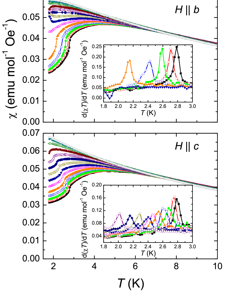
Figure 2: (Color online) Susceptibility of PbCuSO₄(OH)₂ for magnetic fields between 0.5 and 7 T parallel to the crystallographic $a_{\perp}$, $b$, and $c$ direction in the temperature range from 1.8 and 10 K. The insets depict the temperature derivative of the product $\chi T$ for selected field values used to determine the transition temperature $T_{\text{N}}$.

In Fig. 2, we present the temperature dependence of the macroscopic susceptibility of linarite for several magnetic fields $H\parallel a_{\perp}$, $b$, and $c$, respectively. Here, the susceptibility was measured in the temperature range from 1.8 K up to 10 K, while the magnetic field was varied from 0.5 to 7.0 T. For small magnetic fields, the susceptibility has two characteristic features: a broad maximum at around 5 K and a pronounced kink around 2.8 K Wolter et al. (2012). The maximum is common to low-dimensional spin systems and is associated to magnetic correlations within the Cu chains. Further, the kink denotes a transition into a long-range magnetically ordered state at the critical temperature $T_{\text{N}}$.

To determine the transition temperature as a function of the magnetic field, the derivative d($\chi$$T$)/d$T$ has been calculated for each field (see insets in Fig. 2). First, we focus on the direction $H\parallel b$ because for this direction the most remarkable physical properties, with a multitude of field-induced phases, appear. To analyze the data it is helpful to divide the measurements into three regimes: a low-field region from 0–3.0 T, an intermediate region from $\sim$3.0–4.5 T, and a high-field region from $\sim$4.5–7 T. The field dependence of the transition temperature $T_{\text{N}}$ differs from region to region. In the low-field region, $T_{\text{N}}$ monotonously decreases with increasing field. In the intermediate-field as well as in the high-field region the transition temperature changes with different slopes. This observation gives rise to the assumption that for this field direction there appear to be three different distinct types of magnetically ordered phases upon varying the magnetic field.

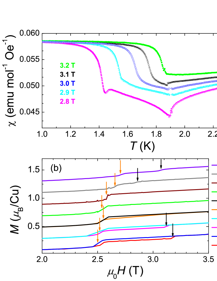
Figure 3: (Color online) (a) Low-temperature susceptibility in different fields for the intermediate-field range of PbCuSO₄(OH)₂ for $H\parallel b$. (b) Field-dependent magnetization of linarite for $H\parallel b$. The steps and hystereses indicate field-induced transitions from the helical ground state to another phase. For clarity the curves are shifted to each other.

In line with this argument, the susceptibility at low temperatures in the low-field region shows an antiferromagnetic-like downturn, while in the intermediate-field region an upturn, and in the high-field region a downturn is observed. This suggests qualitative changes regarding the types of magnetically ordered phases present in linarite for magnetic fields directed along the $b$ direction.

Furthermore, the susceptibility measured in the intermediate-field region to lower temperatures and shown in Fig. 3(a) displays two clear anomalies at 2.8 T. With increasing magnetic field the two transitions are pushed closer to each other, merging at around 3.2 T. Taken together, these observations clearly justify the identification of three different magnetic phases.

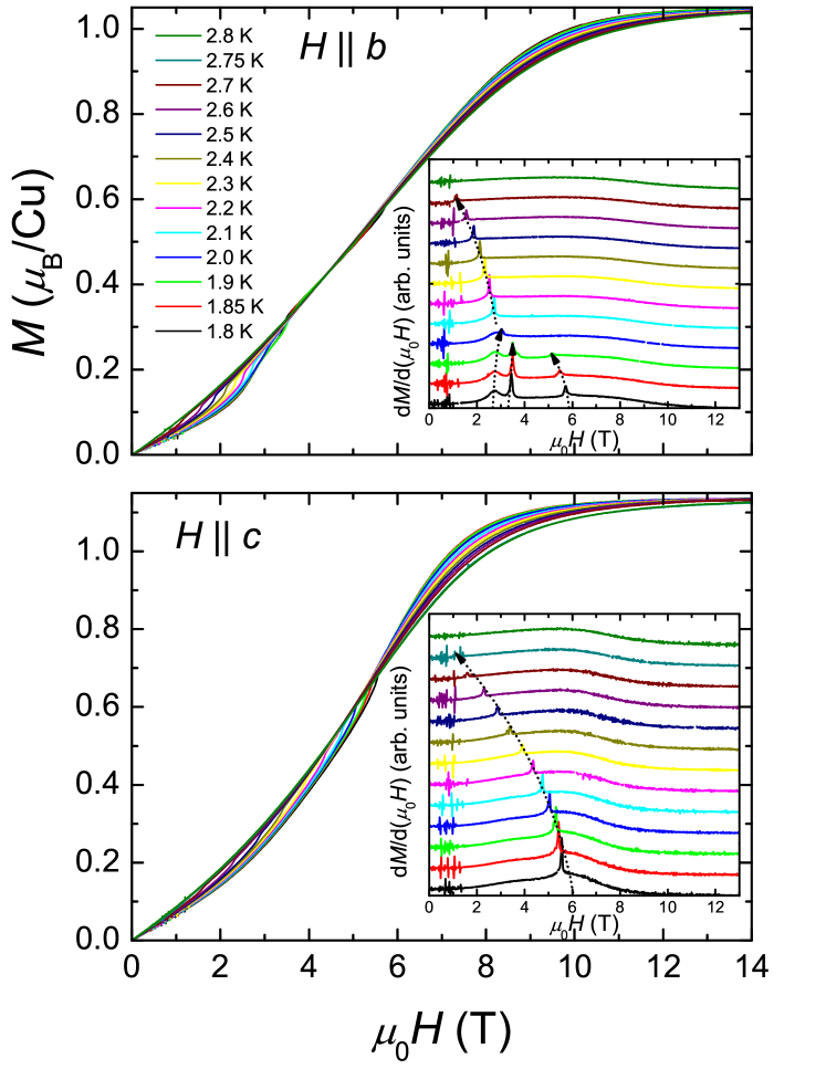
Figure 4: (Color online) Magnetization data, $M(\mu_{0}H)$, and the derivatives d$M$/d($\mu_{0}H)$ of PbCuSO₄(OH)₂ for all crystallographic directions as a function of magnetic field in the temperature range between 1.8 and 2.8 K.

In contrast, for magnetic fields aligned parallel to $a_{\perp}$ and $c$ the susceptibility behaves in a qualitatively similar manner for all magnetic fields. For increasing magnetic fields, the maximum in the susceptibility successively shifts to lower temperatures, indicating a suppression of antiferromagnetic fluctuations, which are gradually replaced by ferromagnetic fluctuations. Moreover, only a monotonous decrease of the magnetic-ordering temperature with increasing field is detected, and the susceptibility always undergoes an antiferromagnetic-like downturn at the transition. Consequently, for these field directions the magnetically ordered phase basically corresponds to the low-field phase for fields $H\parallel b$.

Next, in Fig. 4 we present the magnetization, $M(\mu_{0}H)$, and the field derivatives d$M$/d($\mu_{0}H)$ of PbCuSO₄(OH)₂ as a function of field $H\parallel a_{\perp}$, $H\parallel b$, and $H\parallel c$, respectively, for fixed temperatures between 1.8 and 2.8 K. Measurements were carried out both for increasing and decreasing field to check for hysteretic behavior. Altogether, only a weak hysteresis was observed, depending on the field sweep rate. For small sweep rates, viz., of the order of 0.1 T/min, the hysteresis is negligible. Therefore, here we only show the up-sweep data using quasi-static measurement conditions at small sweep rates.

As reported previously, a large anisotropic response is observed in the saturation magnetization, $M_{\text{sat}}$, and in the saturation field, $H_{\text{sat}}$ Wolter et al. (2012). Here, we focus on the anisotropy of the number of field-induced transitions observed below 2.8 K. Again, as for the susceptibility, the data for $H\parallel a_{\perp}$ and $H\parallel c$ are similar and differ from the data for $H\parallel b$. For $T<2.0$ K and $H\parallel b$, there are three different peaks in the field derivative d$M$/d($\mu_{0}H)$, i.e., at 1.8 K at $\mu_{0}H_{c1}^{b}$ $\approx$ 2.7 T, $\mu_{0}H_{c2}^{b}$ $\approx$ 3.4 T, and $\mu_{0}H_{c3}^{b}$ $\approx$ 5.7 T. With increasing temperature the first transition shifts to higher fields and vanishes at $\sim$2.1 K. As well, the second transition shifts to higher fields and vanishes at $\sim$2.0 K, while the third transition decreases in field and disappears at $\sim$2.0 K. Next, a new peak arises at 2.1 K at about $\mu_{0}H_{c4}^{b}\approx 3.0$ T, which also decreases in field with increasing temperature and fades out at $T_{\text{N}}\approx$ 2.8 K.

In addition, from magnetization experiments for $H\parallel b$ down to 0.25 K a two-step transition, i.e., two anomalies at $H_{c1}^{b}$ and $H_{c2}^{b}$, has been studied. First, by decreasing the temperature from 1.72 K the double transition associated to the intermediate-field phase transforms into a single one at 0.99 K [Fig. 3(b)]. Upon lowering the temperature to less than 600 mK, this intermediate-field regime becomes hysteretic in the magnetization with respect to the field-sweep direction. The transition/hysteretic region is defined by steps in the magnetization indicated by the arrows in the figure. The hysteretic region was also found by magnetocaloric-effect measurements and will be discussed in more detail in section III.3.

The high-field/low-temperature magnetization data (Fig. 5) show that the shift of the third transition to higher fields continues down to temperatures of 0.25 K. Furthermore, the data hint towards the existence of yet another transition in fields of about 9 T, as is indicated by a weak feature in the field derivative of $M(\mu_{0}H)$ (Fig. 5).

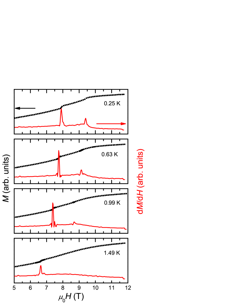
Figure 5: (Color online) High-field magnetization and its field derivative of PbCuSO₄(OH)₂ at low temperatures for $H\parallel b$.

Altogether, the magnetization is in very good agreement with the susceptibility, as again at least three different magnetic phases are observed. In view of the recently discovered helical ground state of linarite Willenberg et al. (2012), the transitions at low fields for $H\parallel b$, $H_{c1}^{b}$ and $H_{c2}^{b}$, could possibly be associated to a spin-spiral reorientation process. Moreover, the features in the magnetization might indicate additional phase transitions or a first-order character of certain transitions. Ultimately, neutron-scattering experiments in these field-induced phases should shed light on these issues B. Willenberg et al. (2014).

For magnetic fields $H\parallel a_{\perp}$ and $H\parallel c$, the derivative of the magnetization only shows one transition, which decreases in field with increasing temperature and vanishes at $T_{\text{N}}$. This magnetic phase corresponds to the ground state phase for $H\parallel b$.

III.3 Specific heat and magnetocaloric effect

The specific heat, $C_{p}$, of PbCuSO₄(OH)₂ was measured in magnetic fields up to 14 T aligned along $a_{\perp}$, $b$, and $c$ between 0.56 and 20 K. Moreover, we also measured $C_{p}$ up to 250 K in zero field (Fig. 6). The open circles represent the measured specific heat, whereas the dotted line represents the estimated phonon contribution, $C_{\text{ph}}$, to the specific heat. The sharp peak in $C_{p}$ at 2.77 K indicates the transition into the long-range ordered magnetic state. Further, a fit $C_{\text{ph}}\propto T^{3}$ does not produce the correct lattice contribution above the transition temperature, since in the temperature range up to $\sim$50 K magnetic fluctuations are present Wolter et al. (2012). Therefore, as a first approximation a simple harmonic model is developed to parameterize the phononic specific heat using one Debye and two Einstein temperatures.

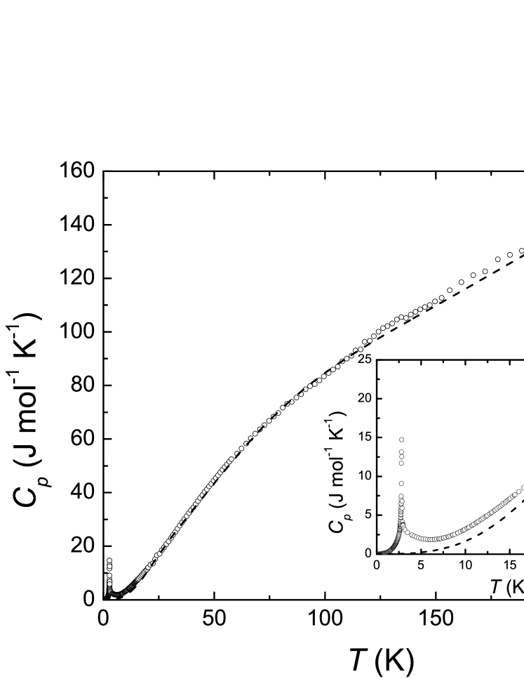
Figure 6: Specific heat of linarite (sample #6) in zero magnetic field. The open circles represent the measured data, the dashed line shows the modelled phononic contribution to the specific heat (for details see text).

Linarite has 11 atoms per elemental formula unit, which implies that 33 vibrational modes to the phononic specific heat exist. Taking into account this constraint, we approximate the lattice contribution to the specific heat by modelling it using one Debye contribution together with two distinct Einstein terms. In Fig. 6, we include the lattice contribution parameterized by using 6 Debye modes with a Debye temperature of $\mathnormal{\Theta_{\text{D}}}=133$ K, 9 Einstein modes with an Einstein temperature $\mathnormal{\Theta_{\text{E,1}}}=292$ K and another 18 Einstein modes with $\mathnormal{\Theta_{\text{E,2}}}=1050$ K.

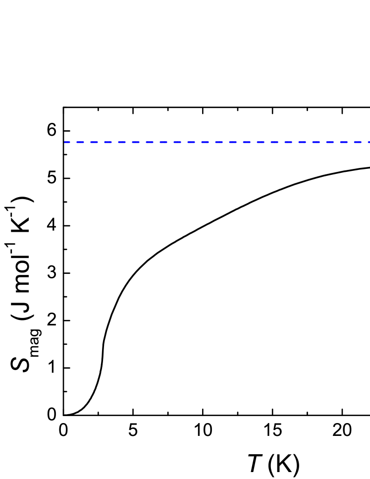
Figure 7: Magnetic entropy of PbCuSO₄(OH)₂ in zero magnetic field. The dashed line corresponds to the expected entropy for a spin-$\tfrac{1}{2}$ system, $R\ln(2)$, while the solid line indicates the entropy derived from the measured specific-heat data.

This parameterization of the lattice specific heat in principle would need an experimental verification by means of for instance inelastic neutron scattering. Most importantly, the obtained key results are not influenced by subtleties in the choice of the modelled lattice contribution, i.e., by the number of Debye and Einstein contributions or by the used absolute values within reasonable error bars. The used parameterization certainly will oversimplify the phonon spectrum, a fact that needs to be taken into account when comparing the experimental specific heat with our theoretical modelling (see below). However, the values derived for $\mathnormal{\Theta_{\text{D}}}$ and $\mathnormal{\Theta_{\text{E}}}$ can be discussed on a qualitative level. Especially, the Debye-like behavior of the lattice specific heat with a rather low value $\mathnormal{\Theta_{\text{D}}}=133$ K is noteworthy in particular in the context of multiferroicity, as it might possibly indicate a significant magneto-elastic coupling in linarite.

Using the lattice contribution to the specific heat, $C_{\text{ph}}$, derived this way, we proceed by determining the magnetic part of the specific heat, $C_{\text{mag}}=C_{p}-C_{\text{ph}}$. Next, we evaluate the entropy of PbCuSO₄(OH)₂ associated with the magnetic contribution in zero magnetic field by calculating the magnetic entropy $S_{\text{mag}}$,

$$S_{\text{mag}}(T)=\int_{0}^{T}\frac{C_{\text{mag}}}{T}\mathrm{d}T,$$ (2)

and which is depicted in Fig. 7. Here, a total magnetic entropy of $S_{\text{mag}}=R\ln(2J+1)=R\ln(2)=5.76$ J mol^-1 K^-1 for Cu spin-$\tfrac{1}{2}$ spins is expected. Experimentally, we obtain $S_{\text{mag}}=5.32$ J mol^-1 K^-1 at $\sim$29.5 K, which is in good agreement with the expectation. This observation represents a consistency check for our estimate of the phonon contribution.

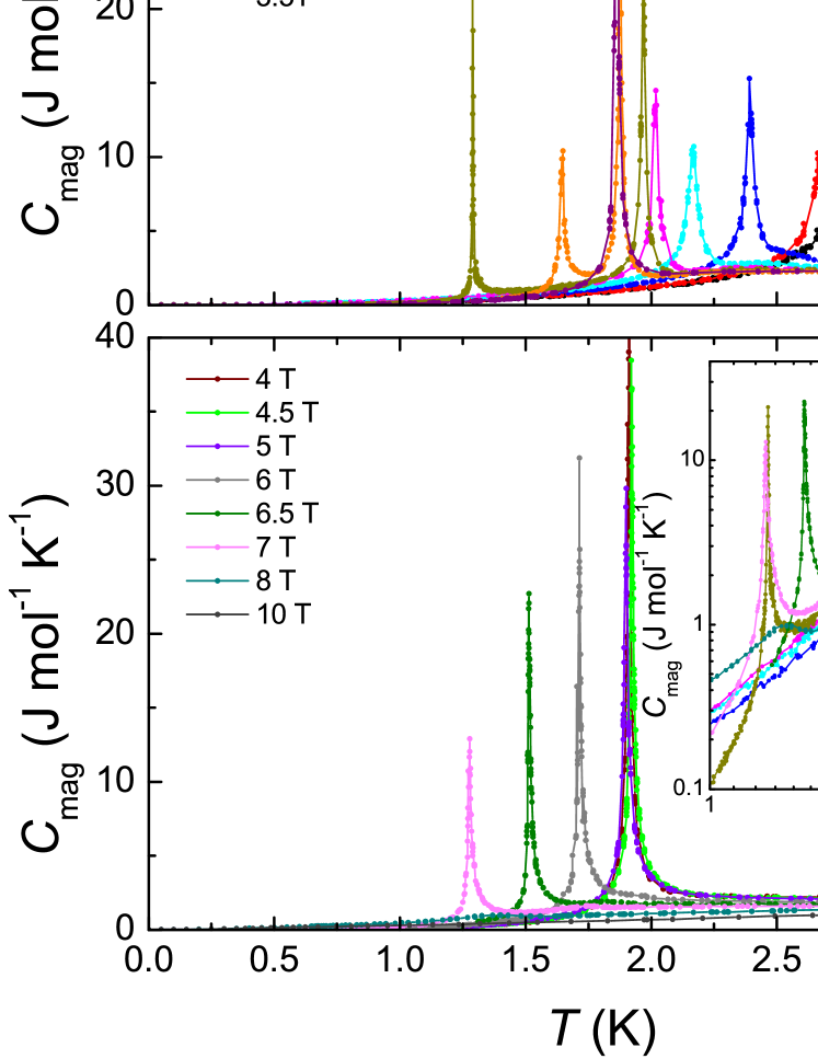
Figure 8: (Color online) Magnetic specific heat of linarite (sample #3) as a function of the magnetic field aligned parallel to $b$. The inset shows data at selected fields on a double-logarithmic scale. The arrow indicates one of the many small anomalies that hint towards another phase transition.

Moreover, from the temperature dependence of $S_{\text{mag}}$ we find that down to $T_{\text{N}}$ there is a remarkable reduction of the entropy. About 75 % of the total magnetic entropy are associated to fluctuations above the magnetic 3D ordering. Such behavior reflects the magnetic low-dimensional character of linarite, with the remaining entropy associated to short-range order and/or quantum fluctuations appearing in the temperature range from above $T_{\text{N}}$ to about $\sim$50 K Wolter et al. (2012).

Further, in Fig. 8 we show the lattice-corrected specific heat for $H\parallel b$ in fields up to 10 T. Here, the upper plot shows the data from 0 to 3.5 T, the lower one the data from 4 to 10 T. From zero field to 2.75 T, the transition temperature decreases with increasing field, while at 3 and 3.25 T an additional peak appears indicating an additional phase transition. At 4 and 4.5 T the transition temperature starts to increase again with field, while it decreases for even higher fields. Furthermore, a hump-like anomaly just prior to this transition into the long-range ordered state is clearly discernible in the field range 2–3 T and 6.5–8 T (see inset of Fig. 8, showing a log-log plot of the data at selected magnetic fields with an arrow to exemplify one transition point). This anomaly appears also to be connected to magnetic correlations which we will discuss below.

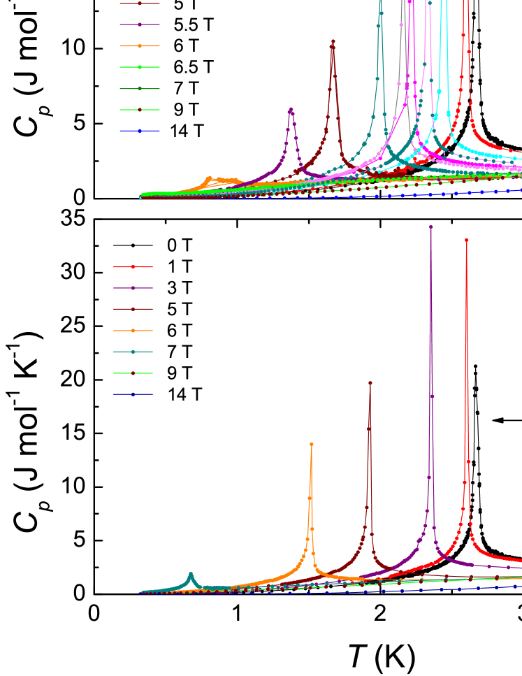
Figure 9: (Color online) Specific heat of linarite (sample #3) as a function of magnetic fields aligned along $a_{\perp}$ and $c$.

For magnetic fields $H\parallel a_{\perp}$ and $H\parallel c$ (Fig. 9), the specific heat shows only one sharp anomaly, which is monotonously shifting to lower temperatures with increasing magnetic field. This anomaly can be attributed to the phase transition into the helical ground state.

Next, in Fig. 10 we present a typical result of a field scan in a magnetocaloric-effect measurement, here for a starting temperature of 1.476 K. In close resemblance to field scans for the magnetization (Fig. 3 and 5), various transitions are visible at 2.65, 2.8, and 6.65 T. The increase in temperature of the up-sweeps and the decrease in temperature at the down-sweeps at the first two transitions indicate that the entropy is reduced above these transitions. In contrast, at the third transition the entropy is increasing. Corresponding experiments have been performed at various temperatures down to 0.3 K (data not shown), allowing the determination of transition fields analogous to those seen in the magnetization study. Moreover, the inset of Fig. 10 enlarges the data at the high-field region. As for to the magnetization experiment at high fields and low temperatures a small feature appears (at about 7.8 T), which shifts to higher fields and becomes more pronounced with lowering the temperature. The fact that we observe features both in the magnetization and in the magnetocaloric effect indicates the existence of another phase transition.

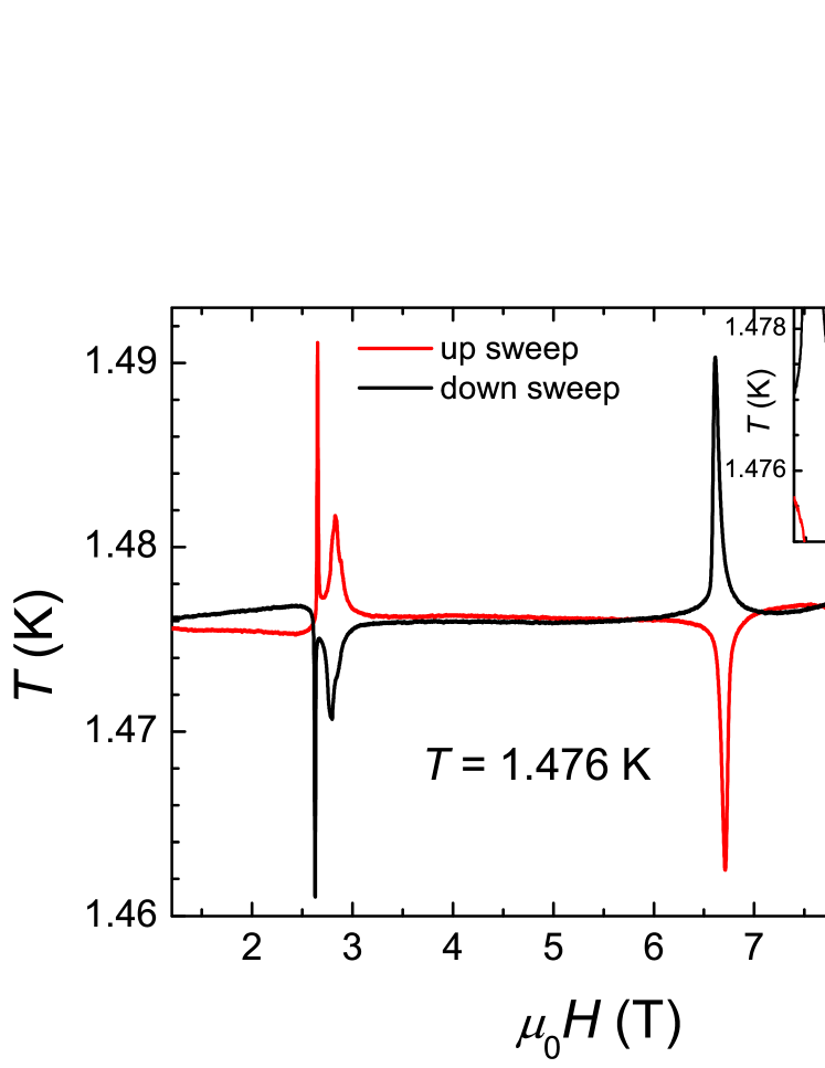
Figure 10: (Color online) Field scan for the determination of the magnetocaloric effect of linarite for $H\parallel b$ at a starting temperature of 1.476 K. The inset enlarges the feature seen in the magnetocaloric effect in high magnetic fields.

Finally, the hysteretic phase at temperatures below $\sim$0.6 K and fields between 2.5 T and 3.2 T observed in the magnetization was also investigated by means of the magnetocaloric effect (not shown). Similar to the magnetization, pronounced and hysteretic features have been observed here which can be associated with a field-induced first-order phase transition.

III.4 Magnetostriction and thermal expansion

In Fig. 11(a) and (b), we display the magnetostriction and thermal-expansion data for magnetic fields $H\parallel b$, respectively. For both experimental techniques the length change of the sample was measured parallel to the $c$ axis using sample #5 in Tab. 1, which has a length of $\sim$0.95 mm at room temperature. The magnetostriction was measured at fixed temperatures between 2.9 K and 2.1 K while varying the magnetic field from 0 up to 16 T. Fig. 11(a) shows the relative length change $\Delta l/l$ as function of the magnetic field. Here, $l$ is the length of the sample at room temperature and $\Delta l$ is the change of the length due to the magnetostrictive effect.

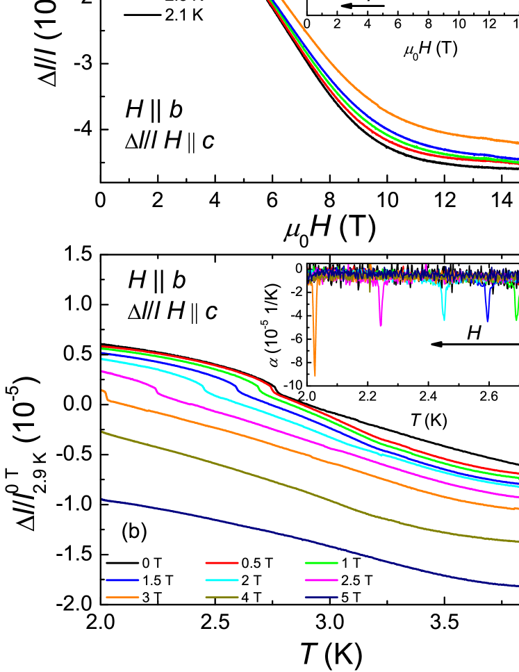
Figure 11: (Color online) (a) Magnetostriction of linarite at various temperatures as a function of magnetic field. (b) The thermal expansion of linarite for various magnetic fields as a function of temperature. The insets depict the field and temperature derivatives $\beta$ and $\alpha$, respectively. Here, the peaks indicate the transition into the long-range ordered ground state.

For all measured temperatures the magnetostrictive effect is negative with increasing magnetic field. Overall, after a strong decrease of $\Delta l/l$ between 0 and 10 T saturation sets in. The transition into the long-range ordered state can be observed as a downward step for temperatures up to 2.7 K. The inset shows the field derivative of the raw data,

$$\beta=\frac{\mathrm{d}}{\mathrm{d}(\mu_{0}H)}\frac{\Delta l}{l},$$ (3)

as a function of the magnetic field. The peaks in $\beta$ indicates the transition into the long-range ordered state, shifting to lower magnetic fields upon increasing temperature. For $T\geq 2.9$ K no transition has been detected.

Next, in Fig. 11(b) the thermal-expansion data are depicted. In this plot, the scale is defined by setting the length change to zero at 2.9 K and 0 T, i.e., the scale is set by $\Delta l/l_{2.9\,\text{K}}^{0\,\text{T}}=(l_{T}^{H}-l_{2.9\,\text{K}}^{0\,\text{T}})/{l_{2.9\,\text{K}}^{0\,\text{T}}}$, in order to illustrate the magnetostrictive effect. The data were obtained in the temperature range from 2.0 to 4.0 K in static magnetic fields up to 5 T. For all investigated magnetic fields, linarite shows a negative thermal-expansion coefficient in the temperature range considered here. The inset shows the derivative

$$\alpha=\frac{\mathrm{d}}{\mathrm{d}T}\frac{\Delta l}{l_{2.9\,\text{K}}^{0\,\text{T}}}$$ (4)

as a function of temperature. Again, the transition temperature is clearly seen as a sharp peak shifting to lower temperature upon increasing magnetic field. For magnetic fields above 3.0 T magnetic long-range ordering occurs below 2.0 K, which is below the temperature range accessible with the present experimental setup.

IV Discussion

IV.1 Magnetic phase diagram

From our experimental data, we derive the magnetic phase diagram for linarite for fields $H\parallel a_{\perp}$, $b$, and $c$. The lower part of Fig. 12 displays the phase diagram for $H\parallel b$, which has already been presented in Ref. Willenberg et al. (2012). Our experiments presented here give evidence for five phases/regions in the phase diagram with different physical properties:

Region I

Region I represents the thermodynamic ground state of linarite, with a helical magnetic order Willenberg et al. (2012) below 2.8 K. This phase is stable for fields up to about 2.7 T at $T=1.8$ K and about 3 T at $T=2$ K (see also the inset of Fig. 4 (middle panel)). This phase boundary can be associated to a spin-flop transition, generic for all CuO₂ chain compounds with a rich phase diagram for the external field applied along the easy axis.

The extrapolated spin-flop field $\mu_{0}H_{\text{SF}}(0)$ at $T=0$ according to the simplest possible phenomenological fit expression

$$\mu_{0}\left[H_{\text{SF}}(T)-H_{\text{SF}}(0)\right]=AT^{\beta},$$ (5)

yields $\mu_{0}H_{\text{SF}}(0)\approx 2.35(6)$ T with $\beta=0.61(15)$. This spin-flop field corresponds to a spin gap $\Delta_{\text{sg}}=3.31$ K or 0.289 meV using $g_{b}=2.1$ derived from our previous ESR data Wolter et al. (2012). From Eq. 5 we estimate 2.64 T for $T=1.2$ K. Also its weak temperature dependence is rather remarkable: a sublinear temperature dependence up to about 2.0 K in our case as compared to a subcubic dependence with $\beta=3.6$ in Li₂CuO₂ up to 5.5 K Lorenz (2011). Noteworthy, both exponents differ from the spin wave prediction $\propto T^{1.5}$ in leading order for a classical unfrustrated cubic antiferromagnet Feder and Pytte (1968).

In the near future we plan a low-temperature ($<1$ K) ESR study for linarite in order to check the value of the spin gap $\Delta_{\rm sg}\approx 0.289$ meV caused by the anisotropic exchange estimated here from the spin-flop field and extrapolated to $T=0$ (see Eq. 5). We believe that the accurate knowledge of $\Delta_{\text{sg}}$ provides a useful constraint for a future refinement of the fundamental anisotropic interactions in the very complex system under consideration as well as for a phenomenological Landau-type free energy functional like in CuO which is expected to be potentially useful for the description of this and other monoclinic multiferroic systems Villarreal et al. (2012); Quirion and Plumer (2013); Bogdanov et al. (2002) (for details see next section).

Region II

Region II exists only at temperatures below $\sim$600 mK, and is defined by hysteresis effects in the magnetization and in the magnetocaloric effect. It does possibly not represent a thermodynamic phase, but a (possible first-order) crossover from one phase to another.

Region III

The phase boundaries of phase III are possibly associated to spin-spiral reorientation processes. Experimentally, we have observed small discrepancies in the boundary positions from measurements on samples from different origins. This indicates that the sample quality/stoichiometry plays some role in this phase. In turn, it reflects the frustrated nature of the magnetic couplings in linarite, with the balance between different magnetic phases being affected by variations of the local magnetic coupling B. Willenberg et al. (2014).

Region IV

Region IV can be divided into two regions, that is above and below $\sim$4.5 T, i.e., region IVa and IVb. While region IVa exhibits a small additional ferromagnetic contribution in the temperature dependence of the magnetic susceptibility at low temperatures, region IVb instead shows an antiferromagnetic contribution. This behavior, together with the pronounced anomalies in the specific heat, suggests that in region IVa a long-range magnetically ordered phase exists, where by canting of antiferromagnetically aligned moments a small ferromagnetic signal is produced. Upon increasing the field to above 4.5 T this ferromagnetic signal is saturated, resulting now in a predominantly antiferromagnetic character of the susceptibility.

Region V

For region V, we find faint anomalies, i.e., a small hump-like features in the specific heat, anomalies in the magnetocaloric effect, and small jumps in the magnetization. The exact nature of the magnetic ordering in region V, however, is unclear. Due to those uncommon small features of the transition, we speculate that short-range magnetic correlations play an important role in this region.

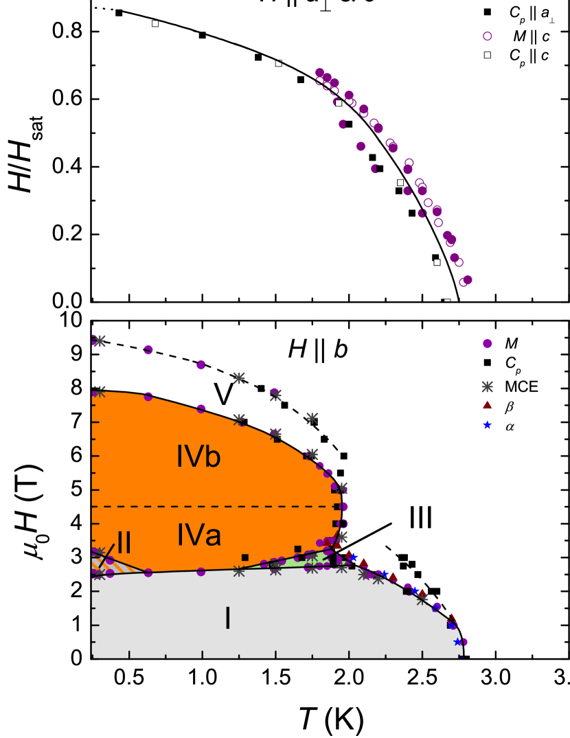
Figure 12: (Color online) Magnetic phase diagram of PbCuSO₄(OH)₂ for $H\parallel a_{\perp}$ and $c$ normalized to $H_{\text{sat}}$ (upper panel) and for $H\parallel b$ (lower panel) Willenberg et al. (2012).

Finally, the upper part of Fig. 12 depicts the phase diagrams derived for fields aligned along $a_{\perp}$ and $c$, respectively, plotted by normalizing the field to the saturation field $H_{\text{sat}}$ for each direction, i.e., $H_{\text{sat}}^{a}=7.6$ T and $H_{\text{sat}}^{c}=8.5$ T Wolter et al. (2012). Here, for both directions only the helical ground state phase of linarite is observed (region I for $H\parallel b$). The scaling for both field directions attests the close similarity of the phase diagrams for these geometries.

IV.2 Linarite in the context of frustrated chain cuprates

So far, about a dozen compounds have been assigned as quasi-1D $s=\tfrac{1}{2}$ Heisenberg systems with competing ferromagnetic nearest-neighbor and antiferromagnetic next-nearest-neighbor intra-chain interactions. However, various fundamental issues such as the existence of multipolar phases or the microscopic origin for multiferroicity have not been comprehensively investigated up to now. To set linarite into a proper context within this challenging family of compounds, we will compare our observations of its magnetic properties and the magnetic phases of linarite with published reports for its magnetically analogous compounds. As we will show, materials comparable to some extent to linarite are LiCuVO₄ Enderle et al. (2005), LiCuSbO₄ Dutton et al. (2012), LiCu₂O₂ Masuda et al. (2004), NaCu₂O₂ Capogna et al. (2005), Li₂ZrCuO₄ Drechsler et al. (2007), Li₂CuO₂ Mizuno et al. (1999), CuO Quirion and Plumer (2013), La₆Ca₈Cu₂₄O₄₁ Matsuda et al. (1996), Ca₂Y₂Cu₅O₁₀ Matsuda et al. (1999), CuGeO₃ Uchinokura (2002), Rb₂Cu₂Mo₃O₁₂ Hase et al. (2004a), Cu(ampy)Br₂ Kikuchi et al. (2000), (N₂H₅)CuCl₃ Maeshima et al. (2003), and Cu₆Ge₆O₁₈$\cdot x$H₂O ($x=0$ and 6) Hase et al. (2004b).

In terms of the type of the magnetic ground state, LiCuVO₄, LiCu₂O₂, NaCu₂O₂, Li₂ZrCuO₄, and CuO have the most in common with linarite. They all exhibit a helically ordered low-temperature phase, with LiCuVO₄ Gibson et al. (2004); Enderle et al. (2005); Schrettle et al. (2008); Svistov et al. (2011), LiCu₂O₂ Masuda et al. (2004); Gippius et al. (2004, 2006); Svistov et al. (2010); Bush et al. (2012), and CuO Giovannetti et al. (2011a); Villarreal et al. (2012); Quirion and Plumer (2013) showing several field-induced phases. In Li₂ZrCuO₄, only a spin-flop transition is observed Tarui et al. (2008), while in NaCu₂O₂ no significant changes of the magnetic properties in an external magnetic field are registered Capogna et al. (2005); Drechsler et al. (2006); Capogna et al. (2010); Leininger et al. (2010).

Thus, the physical properties of LiCuVO₄, LiCu₂O₂, and CuO are closest to those of linarite. In LiCuVO₄, the $\alpha$ value has been discussed controversially. LiCuVO₄ has been described within a pure 1D model Enderle et al. (2010) using two coupling constants, or alternatively by a 3D classical spin-wave model Enderle et al. (2005) using 6 different $J$ values. However, if one only compares the NN and NNN exchange, both models are in good agreement with each other. Originally, Enderle et al. Enderle et al. (2005, 2010) proposed frustration ratios $5.5>\alpha>1.42$, implying a concept of two weakly-coupled antiferromagnetic chains. However, other authors arrived at significantly different frustration ratios $\alpha\approx$ 0.5–0.8 Sirker (2010); Drechsler et al. (2011); Enderle et al. (2011); Nishimoto et al. (2012); Ren and Sirker (2012), implying that a dominant ferromagnetic coupling prevails. LiCuVO₄ undergoes long-range order below $T_{\text{N}}=2.1$ K into a spin-spiral ground state with a propagation vector ${\bf k}=(0,\,0.532,\,0)$ and an isotropic ordered Cu²⁺ moment of 0.31(1)$\mu_{\text{B}}$ Gibson et al. (2004). The saturation field is anisotropic and was determined as 52.1(3) T along the $b$ axis, i.e., the chain direction, 52.4(2) T along $a$ and 44.4(3) T along the $c$ axis Svistov et al. (2011). LiCuVO₄ undergoes transitions into different magnetic-field-induced phases for fields aligned parallel to all crystallographic axes. It is argued that at a critical field, $H_{c1}$, a spin-flop transition from the spiral ground state occurs Büttgen et al. (2007); Nawa et al. (2013). Based on neutron diffraction Masuda et al. (2011) and NMR measurements Büttgen et al. (2012); Nawa et al. (2013), at a second critical field, $H_{c2}$, a transition into a collinear spin-modulated structure is proposed. However, this scenario is contested by recent neutron scattering experiment, which is interpreted in terms of quadrupolar correlations Mourigal et al. (2012). Finally, at $H_{c3}$ a transition into a spin nematic phase has been proposed to occur Zhitomirsky and Tsunetsugu (2010); Svistov et al. (2011); Mourigal et al. (2012). For magnetic fields along the $c$ axis, the phase boundary at $H_{c2}$ could not be investigated so far, which is attributed to anisotropy effects Banks et al. (2007); Büttgen et al. (2007); Schrettle et al. (2008); Svistov et al. (2011).

In LiCu₂O₂, the magnetic exchange paths are still a matter of debate. In Refs. Masuda et al. (2004, 2005), a frustrated double-chain system with large interchain interactions is favored ($\alpha=0.54$). Conversely, Refs. Gippius et al. (2004); Maurice et al. (2012) support a scenario with comparable values for the NN- and NNN-interactions ($\alpha\approx 0.73$) and significantly smaller interchain interactions, leading to a frustrated single-chain derived compound with significant interchain coupling in the basal plane. LiCu₂O₂ undergoes a two-stage transition into a long-range ordered state below $T_{c1}=24.6$ K and $T_{c2}=23.2$ K Roessli et al. (2001); Zvyagin et al. (2002). An incommensurate magnetic ground state with a propagation vector ${\bf k}=(0.5,\,0.174,\,0)$ has been established Masuda et al. (2004), whereas the spin arrangement could not be resolved so far. Masuda et al. Masuda et al. (2004) favor a cycloidal spiral modulation along the chain direction with spin spirals lying in the $ab$ plane. Park et al. Park et al. (2007) suggest a spin spiral propagating in the $bc$ plane. Finally, Kobayashi et al. Yasui et al. (2009); Kobayashi et al. (2009) describe the ground state by assuming an ellipsoidal spin helix in the $ab$ plane with a helical axis tilted by $\sim$45^∘ from the $a$ or $b$ axis, a view supported by Zhao et al. Zhao et al. (2012). The saturation field is estimated to be $\sim$110 T Bush et al. (2012).

LiCu₂O₂ has four highly anisotropic ordered phases. For magnetic fields applied along the $b$ axis, i.e., the chain direction, all four different phases appear: The helical ground state below $T_{c2}$ and a field induced, hysteretic phase above $H_{c1}$ which is interpreted as a spin-flop transition showing pronounced sample dependencies Svistov et al. (2009); Bush et al. (2012). On the other hand, in Ref. Sadykov et al. (2012) the absence of a sharp reorientation transition was instead interpreted in terms of a gradual rotation of the spinning plane of the spiral. The intermediate phase between $T_{c1}$ and $T_{c2}$ is ascribed to a collinear, sinusoidal structure with the spin direction along the $c$ axis Yasui et al. (2009); Kobayashi et al. (2009). Above $H_{c2}$ (which is less anisotropic) another field-induced phase appears and is discussed in the context of a collinear spin-modulated phase similar to that in LiCuVO₄. For fields aligned along the $c$ axis, the spin spiral changes the direction of its spinning plane, viz., does not undergo a spin-flop transition but enters directly, into the supposed collinear spin-modulated phase Sadykov et al. (2012). Along the $a$ axis, the intermediate ordered phase between $T_{c1}$ and $T_{c2}$ is absent but the sequence of the field-induced phases is similar to that for $H\parallel b$ Bush et al. (2012).

In comparison to these cases, in linarite ($\alpha=0.36$) the ordered moment in the helical phase below $T_{\text{N}}\approx 2.8$ K varies from 0.638$\mu_{B}$ in the $ac$ plane to 0.833$\mu_{\text{B}}$ along the $b$ direction, according to the propagation vector ${\bf k}=(0,\,0.186,\,0.5)$ of the spiral Willenberg et al. (2012). The Hamiltonian used to model linarite so far contains two $J$ values and yields better results if some anisotropy is included Wolter et al. (2012). The saturation field is a factor of $\sim$5 (12) smaller than in LiCuVO₄ (LiCu₂O₂) and even more anisotropic. Linarite shows five different magnetic field-induced regimes down to 250 mK, but for fields along the $b$ axis only. The advantage regarding linarite as compared to LiCuVO₄ or LiCu₂O₂ is that all magnetic phases can be accessed in field-dependent neutron-scattering experiments, which allows a direct measurement of the nature of the ordering in the high-field phases. In turn, linarite is an ideal material for testing the scenarios also put forward to describe the high-field phases in LiCuVO₄ and LiCu₂O₂ as well as serves to refine the underlying commonly used isotropic AFM Heisenberg Hamiltonian, e.g., by the inclusion of different spin anisotropies.

On the other hand, from a theoretical point of view, the complex magnetic phase diagram of CuO seems to be closely related to the one of linarite. CuO contains a three-dimensional network of alternately stacked edge-shared CuO₂ chains coupled directly by their edges. As a result of that stacking, buckled corner-shared CuO₃ chains with a large antiferrmoagnetic NN-exchange integral are formed, too (see Fig. 1 in Ref. Rocquefelte et al. (2012)). Noteworthy, the behavior of CuO is somewhat similar to that of the chains considered here for linarite, when the magnetic field is applied along the easy axis (see Fig. 7 of Ref. Quirion and Plumer (2013)). CuO contains six phases among them two spiral/chiral phases, denoted as AF2 and HF2 in Ref. Villarreal et al. (2012) with the spiral propagation along the easy axis for the AF2 phase as in our case.

According to Ref. Rocquefelte et al. (2012) the $J_{1}$ of CuO is antiferromagnetic (at a relatively large Cu-O-Cu bond angle of 96^∘) and the pitch of the spiral should be obtuse, i.e., $\pi/2<\phi<\pi$ in contrast to the acute pitch of linarite. In this case, no multimagnon bound states as low-lying excitations are expected for CuO in sharp contrast to such a possibility left still for linarite (see Sect. V). Also the large AFM interchain coupling for the former would exclude multipolar phases even for change of sign of the NN interaction to be predicted for high pressure Rocquefelte et al. (2012). However, the authors of Ref. Jin et al. (2012) stress the important role of the frustrating NN and NNN intrachain couplings in the stabilization of the spiral state. In general, the situation with respect to the assignment of the numerous exchange couplings involved is still under debate even in the isotropic approach Filippetti and Fiorentini (2005); Jin et al. (2012); Giovannetti et al. (2011a); Rocquefelte et al. (2011); Giovannetti et al. (2011b); Pradipto et al. (2012). With respect to the anisotropic exchange, to the best of our knowledge first of all the importance of the antisymmetric Dzyaloshinskii-Moriya coupling has been discussed Tolédano et al. (2011); Giovannetti et al. (2011a); Pradipto et al. (2012) whereas the symmetric anisotropic exchange has been supposed to be weaker Tolédano et al. (2011). However, a dominant Dzyaloshinskii-Moriya interaction would remove the observed spin gap (spin-flop) Benyoussef et al. (1999) in contrast to the available experimental data for CuO Villarreal et al. (2012); Quirion and Plumer (2013). A more detailed comparison of commonalities and differences of the two similar magnetic phase diagrams of linarite and CuO is postponed to a future publication.

V Theoretical Aspects

In this section, we discuss some theoretical aspects of the one-dimensional isotropic $J_{1}$-$J_{2}$ model and its generalizations to include interchain coupling and exchange anisotropy in the light of the parameter region suggested by the experimental studies described above and in Ref. Wolter et al. (2012). In particular, the effect of an external magnetic field on the specific heat within 1D models will be discussed. Thereby, the main aim is to understand to what extent such simplified effective models are meaningful for the interpretation of the experimental data reported here and to provide an outlook for future generalizations, where it will be necessary. Here we show also results without a direct one-to-one correspondence to our experimental results. These theoretical data are of interest for the community working in the field of theoretical quantum magnetism. This concerns mainly the field dependence of the magnetic specific heat of the isotropic 1D $J_{1}$-$J_{2}$ model. To the best of our knowledge this problem has not been studied systematically in the literature. In this context, we admit that the present state of the art of theory for a rigorous description at arbitrary external magnetic fields at any finite temperature doesn’t allow to answer the corresponding question about the nature of the individual phases shown in the phase diagram in Fig. 12. At the moment for many physical quantities reliable theoretical predictions can be done for high magnetic fields which equal the saturation fields and at $T=0$ or at very low temperature.

First, we consider the isotropic $J_{1}$-$J_{2}$ model. We apply two techniques: (i) the exact diagonalization (CED) for relatively large finite periodic rings with $N$ = 16, 18, 20, and 22 sites formally valid for any temperature but still affected by finite-size effects manifesting themselves for instance in artificially small gaps leading to an incorrect description at very low $T$ and (ii) the transfer matrix renormalization group (TMRG) technique Wang and Xiang (1997); Shibata (1997) which treats the infinite-chain limit at not too low temperature. In the present calculations this lower limit is given by $10^{-3}|J_{1}|$, i.e., of about 0.1 K, still below the lowest available experimental data at 0.25 K and the theoretical results presented recently in Ref. Huang et al. (2012).

In order to estimate the magnitude of the magnetic contribution to the total specific heat and to evaluate the validity of the above modelled harmonic lattice contribution, we start with the calculated temperature dependence (in units of $|J_{1}|$) of the magnetic entropy shown in Fig. 13. Adopting $J_{1}=-94$ K and $\alpha=0.36$ derived from our previous susceptibility fits Wolter et al. (2012), we arrive at $S\approx 0.55$ at $\sim$20 K which is still far from the high-$T$ saturation limit $\ln(2)\approx 0.693$ (in units of $R$) or 5.76 J mol^-1 K^-1 in absolute units. Even at and slightly above 100 K this value is still by far not reached. Naturally, this behavior is more pronounced for somewhat larger $|J_{1}|$ values which provide a reasonable description of the saturation field: $|J_{1}|\approx 118.5(65)$ K, which is shown in the upper panel of Fig. 14. The exact value of $J_{1}$ plays no essential role in these considerations. For a refined estimate the reader is referred to the discussion of the saturation field given below. Returning to the lower panel of Fig. 14 we show our extracted empirical lattice part, too. One realizes a good description above about 3 K, i.e., slightly above the magnetic ordering temperature of 2.8 K, and below about 10 K.

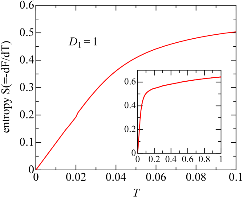
Figure 13: (Color online) Low-temperature $T$-dependence of the magnetic entropy for an 1D isotropic $J_{1}$-$J_{2}$ chain. The temperature is measured in units of $|J_{1}|$. Inset: the same as in the main figure on a larger temperature scale comparable with $J_{1}$. The behavior for $T\rightarrow 0$ has been extrapolated linearly to $T=0$ using the lowest available numerical TMRG data (in between $T=0.006$ and 0.012) as suggested by the adopted scenario of interacting spinons (see text).

The overestimation of the experimental entropy by the theoretical curve (based on a single-chain approach) at low temperatures shown at low temperatures in Fig. 14 is rather natural, because a pure 1D system on the spiral side exhibits no magnetic ordering and hence its entropy must exceed that of the magnetically ordered system at $T\rightarrow 0$. If the picture of interacting spinons (living on the legs of the equivalent zigzag-ladder and interacting via $J_{1}$) might be applied for that case, a linear specific heat $C=\gamma T$ and correspondingly also a linear entropy $S=\gamma T$ can be expected in that limit, whereas in the ordered case dimensionality dependent higher power-laws (quadratic and cubic in 2D and 3D cases, respectively) are expected, which cause a faster decrease of the entropy at low-temperature rem (b).

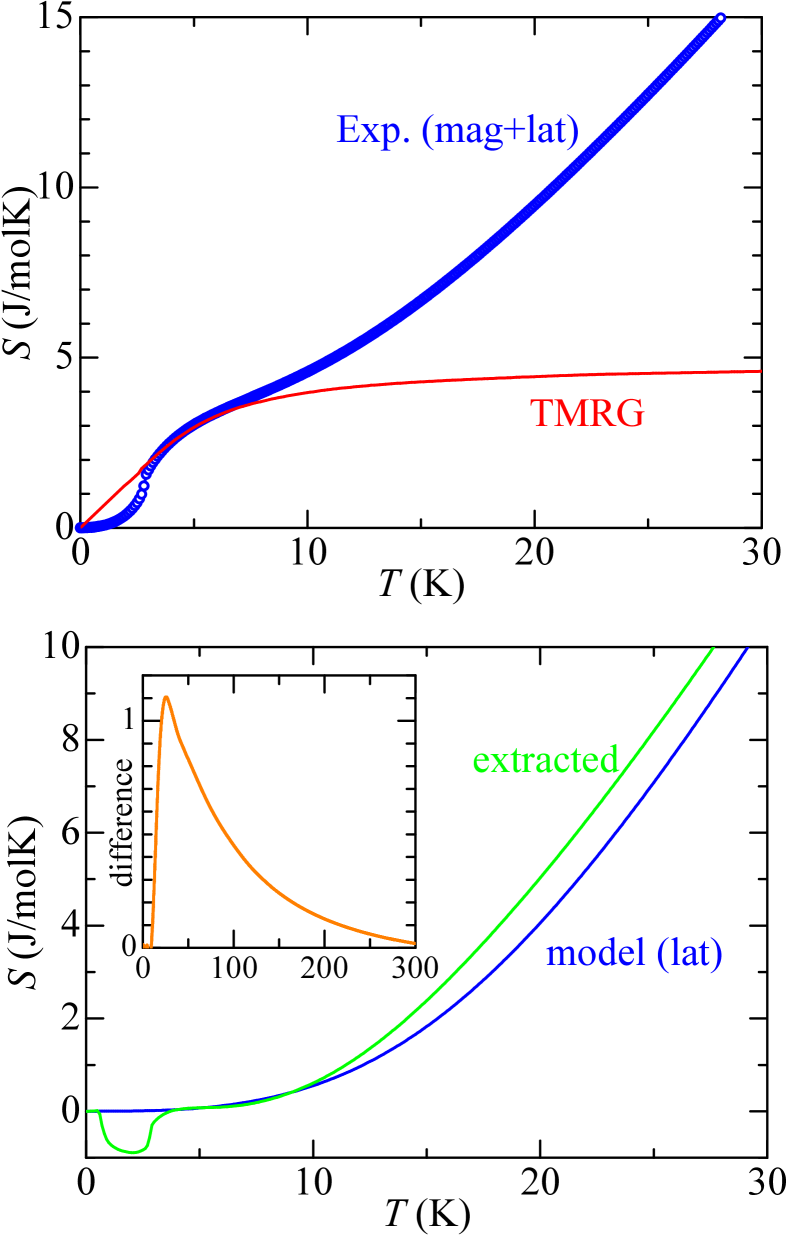
Figure 14: (Color online) Upper panel: Temperature dependence of the magnetic entropy for a 1D isotropic $J_{1}$-$J_{2}$ chain as compared with the measured total entropy including the lattice contribution. Lower panel: The phenomenological lattice contribution resulting from a subtraction of the theoretical 1D contribution shown in (a) from the measured total one as compared with that from a harmonic-lattice model explained in the text. Since the behavior of the theoretical curve for $T\rightarrow 0$ has been extrapolated linearly to $T=0$ (see also the note in the caption of Fig. 13), the difference becomes artificially negative in the region with magnetic ordering at $T<T_{\text{N}}\approx 2.8$ K where the 1D model naturally fails. Inset: difference between the calculations and the above mentioned harmonic model with one Debye spectrum and two Einstein modes.

In fact, the experimentally observed $T^{3}$ dependence below $T_{\text{N}}$ (not shown) further confirms the expected 3D ordering already deduced from previous neutron-diffraction data Willenberg et al. (2012). Thereby, the total cubic term below $T_{\text{N}}$ is found to exceeds very much the Debye contribution to the harmonic lattice term obtained from the fit at $T>T_{\text{N}}$. Approaching the critical point, the low-temperature maximum of the specific heat and the inflection point below it are down shifted to $T=0$, and $\gamma$ monotonously increases. In our case for $\alpha=0.36$, i.e., well above the critical point at $\alpha_{c}=0.25$, a remarkably strong renormalization of the Sommerfeld coefficient already of the order of 30 as compared to the case of non-interacting “leg” spinons for $J_{1}=0$ (i.e. $\alpha=\infty$) can be estimated. A more quantitative analysis of the $J_{1}$ effect will be considered elsewhere.

Above 10 K systematic deviations occur which point to a more soft and/or anharmonic lattice model. In fact, the zig-zag structure of hydrogen pairs along the chain might be interpreted as an “anti-ferroelectric” pseudo-spin ordering of hydrogen positions described within interacting double-well potentials. The observation that the intrachain exchange interactions are strongly dependent on the actual hydrogen positions points to a strong spin pseudo-spin interaction. This situation is reminiscent of the case of Li₂ZrCuO₄ Moskvin et al. (2013); Vavilova et al. (2009) and of CuCl₂ Schmitt et al. (2009) where the pseudo-spin in the former case results from the much heavier Li ions. In the present case of light hydrogens even much stronger quantum effects might be expected. In such a case the subdivision into a magnetic and a lattice part might be difficult in general. However, below 10 K just where the low-$T$ maximum occurs at least a qualitatively correct description might still be expected. The behavior below 3 K seems to be dominated by the interchain coupling ignored in this simple calculation.

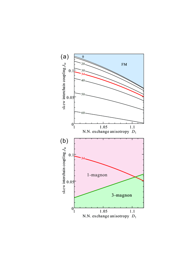
Figure 15: (Color online) Influence of the interchain coupling $J_{\text{ic}}$ and the easy-axis exchange (spin) anisotropy $D_{1}$ of the ferromagnetic (FM) inchain NN-coupling $J_{1}$ on the ground state of a system of coupled anisotropic $J_{1}$-$J_{2}$ spin chains, cf. Eq. 1, for an intrachain frustration rate $\alpha=-J_{2}/J_{1}=0.36$. Upper panel (a): Zero-field plot of the interchain coupling $J_{\text{ic}}$ vs. easy-axis anisotropy $D_{1}$ for various fixed pitch angles $\phi$ (given in degrees at the left side of each curve). The FM ground-state phase (i.e., $\phi=0$), present for large enough $J_{\text{ic}}$, is shown in the light blue upper part of the figure. The NNN-coupling $J_{2}$ is isotropic (i.e., $D_{2}=1$). Note that the red curve corresponds to the observed pitch for linarite. Lower panel (b): Character of the lowest excitations above the FM state for large external field above the saturation field applied in the easy-axis (b) direction. These two figures, which have been slightly modified for clarity here, are taken from S. Nishimoto et al. Nishimoto et al. (2013).

The experimentally obtained pitch angle $\phi$ for linarite of about 33–34^∘ is also strongly affected by the interchain coupling and exchange anisotropy Willenberg et al. (2012); Nishimoto et al. (2013). From this, we estimate a 2D saturation field of $9.5(6)$ T at $T=0$, ignoring the very weak interchain coupling in the third direction and taking $g=2.1$ derived from recent ESR data for the magnetic field parallel to the $b$ axis. This number is in perfect agreement with the experimental value of about 9.5 T (see the upper panel of Fig. 5). Thereby, $J_{1}=-112.6$ K is the lower bound for $J_{1}$ (taking into account the theoretical error bars $\pm 6.5$ K from the $J_{1}$ estimate mentioned above). It has been employed in order to minimize as much as possible the discrepancy in the high-temperature entropy estimated from the applications of the harmonic lattice model and of the theoretical approximation, respectively. In the latter we used in addition to both 1D couplings a skew (first diagonal) antiferromagnetic interchain interaction of 5.6 K and a 12 % easy-axis anisotropy for $J_{1}$ in order to have the correct pitch and a three-magnon phase for an external magnetic field which equals the saturation field and which is directed along the easy axis ($b$ axis) at $T=0$ (see Fig. 15). At such a field the system is fully ferromagnetically polarized. Thereby, it is expected that a similar diagram also holds for some slightly weaker fields and at finite but low temperature. The latter $|J_{1}|$ values are slightly smaller than the estimate given in our previous work for $|J_{1}|\approx 138$ K and a 10 % easy-axis anisotropy together with an interchain coupling of 5.25 K derived from the susceptibility data (see Fig. 16 in Ref. Wolter et al. (2012)). However, considering some uncertainty due to the final field value in the susceptibility measurements and the approximate RPA treatment of the interchain couplings in analyzing the 3D $\chi(T)$ data, the direct estimate of $J_{1}$ from the measured (extrapolated to $T=0$) saturation field is regarded to provide a more accurate value.

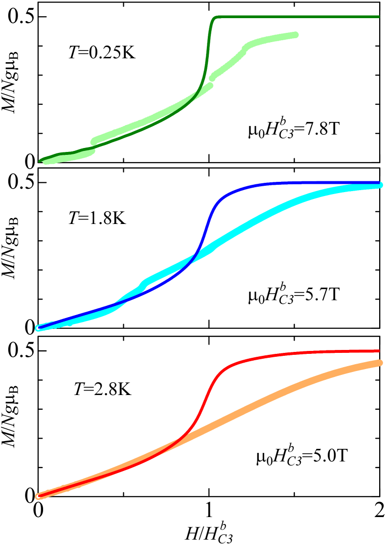
Figure 16: (Color online) Magnetization at finite temperature for an effective single chain (1D) $J_{1}$-$J_{2}$ model for the frustration ratio $\alpha=-J_{2}/J_{1}=0.365$ as compared with the experimental data for $H\parallel b$. $H_{c3}$ is a fit parameter in order to get a reasonable description at low fields. $H_{c3}$ corresponds approximately to the inflection points of the experimental magnetization curves shown in Figs. 4 and Fig. 5.

The inspection of the interchain coupling vs. exchange anisotropy “phase diagram” shown in Fig. 15 clearly demonstrates that a significant symmetric exchange anisotropy of at least of about 10 % is necessary to stabilize a multipolar-(octupolar) phase (three-magnon bound phase). For details of the DMRG-based calculations see Ref. Nishimoto et al. (2010). In this context it is noteworthy that a significant exchange anisotropy suppresses quantum fluctuations and this way contributes to the relatively large magnetic moments observed in the spiral state (see Ref. Willenberg et al. (2012)) in spite of the pronounced quasi-1D state with weak interchain coupling considered here. Thus, we may conclude that a region near the top of the phase V or at very low temperature in the experimental phase diagram shown in Fig. 12 is in fact the place where one has still some chance to detect such an exotic octupolar phase not yet observed for any other real material to the best of our knowledge. Further theoretical studies of even more complex spin chain models and more detailed experimental studies are necessary to settle this issue being of considerable theoretical interest.

Now, we reconsider the $T$ dependence of the magnetization for the magnetic field $H\parallel b$ (see Fig. 16). The inspection of Fig. 5 (upper panel) at low fields reveals that the weak somewhat smeared kink in the experimental curve at the lowest temperature of $T=0.25$ K where data are available corresponds approximately to the spin-flop field of about 2.46 T according to Eq. 5. Let us now turn to an effective isotropic 1D $J_{1}$-$J_{2}$ model. In general, a renormalization of the effective $\alpha$ is expected due to the effects of the interchain coupling and due to the easy-axis anisotropy present in the material but ignored in our 1D model. Since the saturation field is enhanced by the presence of antiferromagnetic interchain interactions a smaller effective $\alpha$ than the more “microscopic” one which enters a 2D or 3D model is expected in order to compensate that enhancement. From the presence of the easy-axis anisotropy just the opposite is expected because it lowers the saturation field, resulting in an overestimation of the effective $\alpha$. Hence, the obtained effective $\alpha_{\text{eff}}=0.365$ points to an approximate compensation of both competing influences with a slightly larger effect from the easy-axis anisotropy. The inspection of Fig. 16 demonstrates that only at high-fields exceeding the saturation field a sizable $T$ dependence is visible. The stronger deviations as compared to the hard-axis case shown in our previous paper Wolter et al. (2012) points again to the importance of anisotropy effects. In this context the presence of antisymmetric contributions as given by the Dzyaloshinskii-Moriya interaction (allowed by the low symmetry of the crystal structure of linarite) may be assumed. However, the examination of such interactions is beyond the scope of the present paper.

Next, we consider the temperature dependence of the magnetic specific heat at ambient external magnetic fields. The results are shown in Fig. 17. The zero-field magnetic specific heat of the 1D $J_{1}$-$J_{2}$ model exhibits a well-known two-peak structure (see e.g. Fig. 5 in Ref. Huang et al. (2012) for $\alpha=0.4$) in a relatively broad region above Huang et al. (2012); Lu et al. (2006) and below Härtel et al. (2008, 2011) the critical point at $\alpha=0.25$. Thereby, for $\alpha>\alpha_{\text{c}}$ the peak at low-temperature shifts towards $T=0$ approaching $\alpha_{c}$. In the present case the high-temperature peak occurs near 0.66$|J_{1}|$ (not shown) whereas the low-temperature peak occurs near 0.032$|J_{1}|$ within a pure 1D model, which corresponds to about 3 K for $|J_{1}|=94$ K mentioned above. Within the anisotropic easy-axis model one finds a tiny down-shift up to 0.026$|J_{1}|$, i.e., to 2.9 K assuming the larger $|J_{1}|\approx$ of 112.6 K derived from the saturation fields discussed above [see panel Fig. 17(c)].

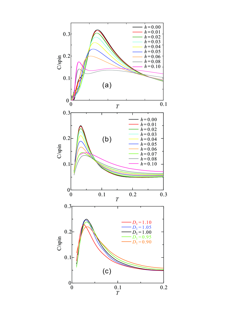
Figure 17: (Color online) Temperature (in units of $|J_{1}|$) dependence of the magnetic specific heat of a single chain within the $J_{1}$-$J_{2}$ model. (a) Complete diagonalization-based calculations for periodic rings with $N=22$ sites for different dimensionless magnetic fields $h=gH/|J_{1}|$. (b) The same as in (a) for TMRG calculations. (c) $T$ dependence of the magnetic specific heat at zero magnetic fields but with symmetric anisotropic exchange included. $D_{1}>1$ means easy-axis anisotropy for $J_{1}$, see Eq. 1. $D_{1}=1$ corresponds to the isotropic limit of the $J_{1}$-$J_{2}$ model as shown in (b), too

.

The comparison of the behavior of the (3D solid) linarite with the properties of the 1D models given above can be justified (at least on a qualitative level) by a random phase approximation like approach. Then such a correspondence is based on the knowledge that a phase transition near the critical point due to finite interchain coupling is triggered also by the sharp, well pronounced low-temperature peak in the specific heat in the 1D component. Thus, we have compared the somewhat broader peaks of the 1D-models with the sharp peaks corresponding to the field dependent phase transitions in the compound under considerations. Experimentally, at ambient fields the magnetic phase transition takes place at 2.8 K. We ascribe that slightly smaller value as compared to theoretical values of the peaks in the 1D models at 2.9 K and 3 K mentioned above to the effect of weak interchain coupling ignored in both 1D approaches.

Finally, we summarize briefly the influence of the exchange anisotropy on the magnetic specific heat [see Fig. 17(c)]. The account of a sizable easy-axis anisotropy for $J_{1}$ leads to a down-shift of the low-temperature maximum and to a sharpening of its peak. In the easy-plane case the opposite behavior is observed. In both cases the discrepancy with the harmonic model is not removed which suggests once again that the reason for the discrepancy between an effective and the simple harmonic model is not on the magnetic side but on the lattice model side.

We conclude this section with a critical comparison of both theoretical methods we have employed to calculate the temperature dependence of the magnetic specific heat. Considering the results of our finite-cluster calculations using the spectrum obtained by the CED depicted in Fig. 17(a), one realizes an observable down-shift of the peak position down to 0.02 in fields from ambient field to $h=0.06$ (i.e. corresponding to about 5.6 T for $|J_{1}|\approx 119$ K and $g=2.1$, see the definition of $h$ after Eq. 1 to be compared by a much smaller shift obtained by the TMRG calculations). Anyhow, since experimentally a much larger down-shift is observed for 7 T, only, we ascribe that difference to interchain coupling, too. The study of that effect as well as the influence of various exchange anisotropies is postponed to future studies in order to achieve a better quantitative description of the experimental data. For higher fields there is a clear upshift observed both in the CED results for short rings and also within the TMRG (see panel (b)). The appearance of further structures in the $C(T)$ curve (including the second low-temperature peaks for the highest fields, $h=0.08$ and $h=0.1$) below $T\approx 0.02$ in the CED data, see panel (a), is certainly a finite-size artifact of this approach.

VI Summary

In conclusion, we have determined the detailed magnetic phase diagram of linarite by use of comprehensive thermodynamic investigations. For magnetic fields aligned along the $b$ direction, linarite shows a rich variety of magnetic phases. This phase diagram is even more complex than those of the related frustrated spin-$\tfrac{1}{2}$ chain compounds LiCuVO₄ and LiCu₂O₂. However, there are various similarities between the different systems. We found remarkable similarities with the magnetic phase diagram for the also monoclinic and multiferroic CuO proposed very recently in the literature Villarreal et al. (2012); Quirion and Plumer (2013) for the case of an external magnetic field directed along the easy axis. A detailed and comprehensive future comparison of both challenging systems is expected to provide a deeper insight in the role of the frustrated edge-shared CuO₂ chains in their crucial role for the rich anisotropy effects observed here and there. In the case of linarite, because of the relevant magnetic field scales, neutron-scattering experiments will give a much deeper microscopic insight into the magnetic phases and excitations of this material as well as into this class of materials as a whole. Moreover, based on our studies, linarite possibly is a candidate for showing an octupolar (three-magnon) bound states hitherto experimentally unknown. In addition, the expected highly anharmonic oscillatory behavior of hydrogen points to the need for even more complex models of strongly interacting spins and pseudo-spins as the simplest model for the corresponding ferroelectric dipoles in the extreme quantum limit (interacting two-level systems) for the description of the quantum motion of hydrogen ions (protons) in double- or multiple-well lattice potentials. To reach a deeper understanding of these complex and challenging phases and interactions further experimental and theoretical studies are necessary.