Detection of a large sample of $\gamma$ Dor stars from $Kepler$ space photometry and high-resolution ground-based spectroscopy.^,

Abstract

Context. The launches of the MOST, CoRoT, and $Kepler$ missions opened up a new era in asteroseismology, the study of stellar interiors via interpretation of pulsation patterns observed at the surfaces of large groups of stars. These space-missions deliver a huge amount of high-quality photometric data suitable to study numerous pulsating stars.

Aims. Our ultimate goal is a detection and analysis of an extended sample of $\gamma$ Dor-type pulsating stars with the aim to search for observational evidence of non-uniform period spacings and rotational splittings of gravity modes in main-sequence stars typically twice as massive as the Sun. This kind of diagnostic can be used to deduce the internal rotation law and to estimate the amount of rotational mixing in the near core regions.

Methods. We applied an automated supervised photometric classification method to select a sample of 69 Gamma Doradus ($\gamma$ Dor) candidate stars. We used an advanced method to extract the $Kepler$ light curves from the pixel data information using custom masks. For 36 of the stars, we obtained high-resolution spectroscopy with the HERMES spectrograph installed at the Mercator telescope. The spectroscopic data are analysed to determine the fundamental parameters like $T_{\rm eff}$, $\log{g}$, $v\sin{i}$, and [M/H].

Results. We find that all stars for which spectroscopic estimates of $T_{\rm eff}$ and $\log{g}$ are available fall into the region of the HR diagram where the $\gamma$ Dor and $\delta$ Sct instability strips overlap. The stars cluster in a 700 K window in effective temperature, $\log{g}$ measurements suggest luminosity class IV-V, i.e. sub-giant or main-sequence stars. From the $Kepler$ photometry, we identify 45 $\gamma$ Dor-type pulsators, 14 $\gamma$ Dor/$\delta$ Sct hybrids, and 10 stars which are classified as “possibly $\gamma$ Dor/$\delta$ Sct hybrid pulsators”. We find a clear correlation between the spectroscopically derived $v\sin{i}$ and the frequencies of independent pulsation modes.

Conclusions. We have shown that our photometric classification based on the light curve morphology and colour information is very robust. The results of spectroscopic classification are in perfect agreement with the photometric classification. We show that the detected correlation between $v\sin{i}$ and frequencies has nothing to do with rotational modulation of the stars but is related to their stellar pulsations. Our sample and frequency determinations offer a good starting point for seismic modelling of slow to moderately rotating $\gamma$ Dor stars.

1 Introduction

Asteroseismology is a powerful tool for diagnostics of deep stellar interiors not accessible through observations otherwise. Detection of as many oscillation modes as possible that propagate from the inner layers of a star all the way up to the surface is a clue towards better understanding of stellar structure at different evolutionary stages via asteroseismic methods. The recent launches of the MOST (Microvariability and Oscillations of STars, Walker et al. 2003), CoRoT (Convection Rotation and Planetary Transits, Auvergne et al. 2009) and $Kepler$ (Gilliland et al. 2010a) space missions delivering high-quality photometric data at a micro-magnitude precision led to a discovery of numerous oscillating stars with rich pulsation spectra and opened up a new era in asteroseismology.

Besides acoustic waves propagating throughout the stars and having the pressure force as their dominant restoring force (p-modes), some stars pulsate also in the so-called g-modes for which gravity (or buoyancy) is the dominant restoring force. Given that gravity modes have high amplitudes deep inside stars, they allow to study properties of the stellar core and nearby regions far better than acoustic modes.

Table 1: Influence of the pixel mask choice on the frequency analysis for KIC 08364249. The uncertainty in frequency is given by the Rayleigh limit (1/$T$) which amounts 0.0011 d^-1 (0.0127 $\mu$Hz) in this case. The barred values indicate frequencies which are not present when using our custom mask to produce the light curve but are detected when using the standard mask data. The frequencies are sorted according to the amplitude.

Fi	Frequency		Fi	Frequency
	d-1	$\mu$Hz		d-1	$\mu$Hz
F1	1.8693	21.6282	F33	3.8555	44.6083
F2	2.0095	23.2498	F34	0.0318	0.3684
F3	1.9862	22.9802	F35	0.0164	0.1895
F4	1.8893	21.8597	F36	3.9690	45.9208
F5	1.8633	21.5585	F37	1.7565	20.3222
F6	1.9194	22.2069	F38	0.0370	0.4276
F7	0.0202	0.2342	F39	3.8788	44.8779
F8	1.7523	20.2736	F40	1.8684	21.6177
F9	1.9040	22.0293	F41	0.0626	0.7248
F10	0.0123	0.1422	F42	1.7759	20.5471
F11	1.9276	22.3029	F43	3.7388	43.2576
F12	0.0224	0.2592	F44	1.9380	22.4226
F13	0.0182	0.2106	F45	0.0863	0.9984
F14	1.7293	20.0079	F46	0.0079	0.0909
F15	0.0144	0.1672	F47	3.9957	46.2299
F16	1.8701	21.6374	F48	1.9855	22.9723
F17	3.7617	43.5233	F49	0.0283	0.3276
F18	1.8463	21.3612	F50	4.0189	46.4982
F19	1.8314	21.1890	F51	4.0152	46.4561
F20	0.0102	0.1185	F52	0.1203	1.3916
F21	0.1402	1.6217	F53	1.9365	22.4055
F22	2.0642	23.8824	F54	2.0958	24.2480
F23	3.9474	45.6710	F55	1.8825	21.7808
F24	0.0260	0.3013	F56	1.9114	22.1148
F25	0.0297	0.3434	F57	1.9454	22.5081
F26	1.8577	21.4941	F58	3.8523	44.5715
F27	2.0796	24.0613	F59	1.8885	21.8505
F28	1.8926	21.8978	F60	1.7235	19.9408
F29	0.1168	1.3508	F61	1.7716	20.4972
F30	1.8754	21.6979	F62	3.9916	46.1826
F31	0.0648	0.7498	F63	1.9871	22.9907
F32	2.0495	23.7128	F64	2.2176	25.6579

In this paper, we focus on the class of main-sequence, non-radially pulsating stars named after the prototype star Gamma Doradus ($\gamma$ Dor, hereafter), whose multiperiodic variable nature was first reported by Cousins (1992). $\gamma$ Dor stars are assumed to pulsate in high-order, low-degree gravity modes driven by the flux blocking mechanism near the base of their convective zones (Guzik et al. 2000; Dupret et al. 2005). These stars have masses ranging from 1.5 to 1.8 M_⊙ (Aerts et al. 2010) and A7–F5 spectral types (Kaye et al. 1999). They are usually multiperiodic pulsators exhibiting both low-amplitude photometric and spectroscopic variability with periods between 0.5 and 3 days (Kaye et al. 1999). $\gamma$ Dor stars are grouped in a region close to the red edge of the classical instability strip in the Hertzsprung -Russell (HR) diagram. The theoretical $\gamma$ Dor instability strip overlaps with the region where the Delta Scuti ($\delta$ Sct, hereafter) stars pulsating in low-order p-modes are located. Pulsators in the overlapping region are expected to show both high-order g-modes probing the core and low-order p- and g-modes probing the outer layers. Such hybrid pulsators are among the most interesting targets for asteroseismic diagnostics as the co-existence of the two types of oscillation modes yields potential of constraining the whole interior of the star, from the core to the outer atmosphere.

The first-order asymptotic approximation for non-radial pulsations developed by Tassoul (1980) shows that, in the case of a model representative of a typical $\gamma$ Dor pulsator, the periods of high-order, low-degree g-modes are equally spaced. However, the steep chemical composition gradient left by the shrinking core in stars with masses above $\sim$1.5 M_⊙ causes sharp features in the Brunt-Väisälä frequency to occur, which in turn determines how the gravity modes are trapped in the stellar interiors. The trapping also leads to the deviation from uniform period spacing of the g-modes of consecutive radial order $n$ (Miglio et al. 2008). Moreover, the rotational splitting of the g-modes provides a unique opportunity to deduce the internal rotation law and to estimate the amount of rotational mixing that may be partly responsible for the chemically inhomogeneous layer exterior to the core. This type of diagnostic is not available for stars pulsating purely in p-modes. Consequently, a non-uniform period spacing together with the rotational splitting of gravity modes represent a powerful tool for the diagnostics of the properties of the inner core and surrounding layers.

This idea was worked out in full detail for white dwarfs by Brassard et al. (1992) and applied to such type of objects by, e.g., Winget et al. (1991) and Costa et al. (2008). Miglio et al. (2008) developed similar methodology for gravity modes of main-sequence pulsators. Recently, Bouabid et al. (2013) studied the effects of the Coriolis force and of diffusive mixing on high-order g-modes in $\gamma$ Dor stars, adopting the traditional approximation. The authors conclude that rotation has no significant influence on instability strips but does allow to fill the gap between $\delta$ Sct-type p- and $\gamma$ Dor-type g-modes in the frequency spectrum of a pulsating star by shifting the g-mode frequencies to higher values. Bouabid et al. (2013) also conclude that the deviations from a uniform period spacing is no longer periodically oscillating around a constant value, but as far as we are aware this theoretical description was not yet applied to data.

A first concrete application of detected period spacings to main-sequence stars was done by Degroote et al. (2010), based on CoRoT data of the Slowly Pulsating B (hereafter called SPB) star HD 50230. Among some hundreds statistically significant frequencies, the authors identify eight high-amplitude peaks in the g-mode regime showing a clear periodic deviation from the mean period spacing of 9418 s. They link this deviation with the chemical gradient left by the shrinking core and constrain the location of the transition zone to be at about 10 per cent of the radius. Additionally, the authors suggest an extra-mixing around the convective core to occur. Another indication of a non-uniform period spacing was reported by Pápics et al. (2012b) for the SPB/$\beta$ Cep hybrid pulsator HD 43317. The authors detect two series of ten and seven components in the g-mode regime showing mean period spacings of 6339 and 6380 s, respectively. Given that the two values of the period spacing are almost the same, the authors conclude that both series belong to the same value of degree $l$ but have different azimuthal numbers $m$. However, they do not present any physical interpretation of the observed period spacings, claiming that the detected modes are in the gravito-inertial regime, and thus full computations with respect to the rotation of the star, rather than approximations based on a perturbative approach are required.

The class of $\gamma$ Dor-type pulsators should contain both stars with a shrinking and expanding core during their main-sequence evolution, and seismic probing of the core holds the potential to discriminate between those two scenarios. Based on the analysis of almost 11 500 light curves gathered with the CoRoT space mission, Hareter et al. (2010) confidently detect 34 $\gamma$ Dor stars and 25 $\gamma$ Dor/$\delta$ Sct hybrid pulsators with about 50 stars still being candidates of either of the class. For five out of 34 $\gamma$ Dor stars, the authors detect regular patterns of period spacings of high-order gravity modes ranging from 650 to 2 400 s. Hareter (2012) extends the sample up to 95 and 54 $\gamma$ Dor and hybrid pulsators, respectively, and attempts to interpret the period spacings from the previous study. The author finds that the observed spacings are too short to be due to high-order $l=1$ modes and concludes that these spacings are either coincidental due to the rather poor Rayleigh limit of CoRoT data or need some other explanation. Recently, Maceroni et al. (2013) studied an eclipsing binary, CoRoT 102918586, with a $\gamma$ Dor pulsating component based on space photometry and ground-based spectroscopy. The authors detect a nearly equidistant frequency spacing of about 0.05 d^-1 (0.58 $\mu$Hz) which was found to be too small to be due to the stellar rotation. The corresponding mean period spacing of 3110 s was found to be consistent with the theoretical spacings of $l=1$ high-order g-modes based on the models computed without convective overshooting. Neither of the two studies present a detailed modelling of the deviation from the constant period spacings, however, and both rely on comparison with theoretically predicted mean values of the period spacings for an F-type star. This encourages us to start this work, with the aim of studying in more detail the frequency content of $\gamma$ Dor stars observed in the $Kepler$ data, which have a much more suitable Rayleigh limit to unravel the different structures observed in their amplitude spectra.

Our ultimate goal is to deduce with high precision the extent of the stellar core and mixing processes near the core for $\gamma$ Dor-like stars burning hydrogen in their cores. This requires the selection of a large enough sample of slowly to moderately rotating $\gamma$ Dor stars and this paper is devoted to this purpose. Both photometric and spectroscopic data have been acquired and are described together with the data reduction process in Sect. 2. The sample of stars is introduced in Sect. 3. Photometric characterization of the sample is given in Sect. 4, the results of the spectroscopic analysis of all stars for which spectra are available are outlined in Sect. 5. The conclusions and an outlook for future research are given in Sect. 6.

Table 2: Journal of spectroscopic observations. N gives the number of obtained spectra, $V$ – visual magnitude. All spectra have been taken in 2011. The stars are sorted according to the KIC number.

KIC	Designation	$V$	N	Observed
02710594	TYC 3134–1158–1	11.8	4	May – August
03448365	BD+38 3623	9.9	2	May – June
04547348	TYC 3124–1108–1	11.4	4	May – August
04749989	TYC 3139–151–1	9.6	2	May – June
04757184	TYC 3139–499–1	11.7	4	May – August
05114382	TYC 3140–1590–1	11.6	4	July – August
05522154	TYC 3125–2566–1	10.4	3	May – June
05708550	TYC 3139–428–1	11.9	4	July – August
06185513	TYC 3127–2073–1	11.9	4	May
06425437	TYC 3128–1004–1	11.5	3	May
06468146	HD 226446	10.0	2	July
06678174	TYC 3129–3189–1	11.7	4	May – August
06935014	TYC 3128–1500–1	10.9	5	May – June
07023122	BD+42 3281	10.8	4	May – July
07365537	BD+42 3365	9.2	3	May
07380501	TYC 3144–1294–1	12.5	4	July – August
07867348	TYC 3130–1278–1	11.0	4	May
08364249	—–	11.9∗	4	July – August
08375138	BD+44 3210	11.0	4	May – August
08378079	TYC 3148–1427–1	12.5	3	August
08611423	TYC 3132–580–1	11.6	4	May – June
08645874	HD 188565	9.9	2	July
09210943	TYC 3542–291–1	11.8	3	May – August
09751996	TYC 3540–1251–1	11.0	4	May
10080943	TYC 3560–2433–1	11.7	4	August
10224094	TYC 3561–399–1	12.5	4	July – August
11099031	TYC 3562–121–1	10.0	4	July
11294808	TYC 3551–405–1	11.7	4	May – August
11721304	TYC 3565–1474–1	11.7	4	July – August
11826272	BD+49 3115	10.2	3	May – August
11907454	TYC 3550–369–1	11.7	4	May – August
11917550	TYC 3564–346–1	11.1	4	May – August
11920505	TYC 3564–2927–1	9.9	2	May
12066947	TYC 3564–16–1	10.2	3	May – July
12458189	TYC 3555–240–1	11.6	4	May – August
12643786	TYC 3554–1916–1	11.6	4	May – August
∗$Kepler$ magnitude

2 Observations and data reduction

We base our analysis on high-quality photometric and spectroscopic data. The light curves have been gathered by the $Kepler$ space telescope and are of micro-magnitude precision. The data are acquired in two different modes, the so-called $long$ (LC) and $short$ (SC) cadences. In both cases exposure time is 6.54 s of which 0.52 s is spent for the readout. The LC integrate over 270 single exposures giving a time-resolution of 29.42 min whereas one data point in the SC mode contains 9 exposures corresponding to a 58.85-s time resolution. The data are released in quarters ($\sim$ 3 months of nearly continuous observations), the periods between spacecraft rolls needed to keep its solar panels pointing towards the Sun. More information on the characteristics of the SC and LC data can be found in Gilliland et al. (2010b) and Jenkins et al. (2010), respectively.

Figure 1: The target sample representation. The plot illustrates all frequencies we consider as independent ones for all 69 stars. Note the different Y-scales for the two panels.

Figure 2: Light curves (left) and amplitude spectra (right) of selected stars. From top to bottom: KIC 02710594, 03448365, 03744571, 04547348, 04749989, and 10080943. The y-scale of the left panel represents differential magnitude after subtraction of the corresponding mean value for each target. Note mmag scale for KIC 04749989.

For the analysis, we use all data that was publicly available by the time of the analysis (Q0-Q8) and our $Kepler$ Guest Observer data (GO, Still et al. 2011). LC data are well-suited for our analysis as the corresponding Nyquist frequency of 24.47 d^-1 (283.12 $\mu$Hz) is well above the $\gamma$ Dor-typical oscillation periods that lie between 0.5 and 3 days. Instead of using the standard pre-extracted light curves delivered through MAST (Mikulski Archive for Space Telescopes), we have extracted the light curves from the pixel data information using custom masks based on software developed by one of us (SB, Bloemen et al., in prep). Contrary to the standard masks, which only use pixels with the highest signal-to-noise (S/N) ratios, our masks contain as many pixels as possible with significant flux. The light curves obtained by including these lower S/N pixels have significantly less instrumental trends than the standard light curves. Table 1 shows the influence of the proper mask choice on the frequency analysis of one of our $\gamma$ Dor stars. The fifteen crossed out low frequencies present in the standard pre-extracted light curve are gone from the data when we extract the light curve from the pixel data using a custom mask. An appropriate removal of the instrumental effects is essential for $\gamma$ Dor stars pulsating in high-order g-modes that show up in the low-frequency domain. One must thus cautiously interpret frequencies deduced from the standard light curves (as listed in, e.g. Grigahcène et al. 2010; Uytterhoeven et al. 2011; Balona et al. 2011).

We acquired high-resolution spectroscopy for the brightest targets with the HERMES (High Efficiency and Resolution Mercator Echelle Spectrograph, Raskin et al. 2011) spectrograph attached to the 1.2-m Mercator telescope (La Palma, Canary Islands). The spectra have a resolution of 85 000 and cover the wavelength range from 377 to 900 nm. Typical S/N ratios measured at $\lambda\lambda$ 5500 Å are about 40 for each spectrum. An overview of spectroscopic observations is given in Table 2.

The spectra have been reduced using a dedicated pipeline. The data reduction procedure included bias and stray-light subtraction, cosmic rays filtering, flat fielding, wavelength calibration by ThArNe lamp, and order merging. The normalisation to the local continuum has been performed in two steps: first, by fitting a “master function” (cubic spline connected through some tens of carefully selected continuum points) that accounts for the artificial spectral signature induced by the flat field procedure. The spectral signature of the flat field lamps is attenuated by red blocking filters (Raskin et al. 2011) which induces a specific spectral signature in the reduced merged spectra. And second, a correction for small-scale effects by selecting more “knot points” at wavelengths free of spectral lines and connecting them with linear functions. At this phase, all spectra are corrected for their individual radial velocities (RVs) as the position of the selected “knot points” is fixed in wavelength. For more information on the normalisation procedure we refer to Pápics et al. (2012b).

3 The target sample

Our selection of $\gamma$ Dor targets is based on an automated supervised classification method, applied to the entire $Kepler$ Q1 dataset of about 150 000 light curves. For detailed information on the method, we refer to Debosscher et al. (2011). Basically, we summarize the main characteristics of each light curve by means of a uniform set of parameters, obtained from a Fourier decomposition. These include, e.g., significant frequencies present in the light curve, their amplitudes and their relative phases. Statistical class assignment is then performed by comparing these parameters with those derived from a training set of known class members for several types of variable stars. This classification procedure only uses information derived from the $Kepler$ light curve, not sufficient to distinguish all variability types. Therefore, we refined the classification in a second stage by using 2MASS colour information. This way, we could discriminate between pulsating stars showing the same type of variability in their light curves, but residing at different locations in the HR diagram (e.g. $\gamma$ Dor versus SPB pulsators).

In total, we selected 69 $\gamma$ Dor candidate stars. Figure 1 represents the entire sample by showing all frequencies we consider as independent ones (cf. Section 4) for all 69 targets. The total number of shown frequencies is 344, which results from about 5 individual peaks per object. Such low number of independent modes is plain statistical and does not mean that there are only 5 independent, non combination frequencies per star. In any sufficiently large set of frequencies, it is not expected to find more than $\sim$10 (depending on the criteria used to search for combination frequencies) independent modes to occur as there is no way to distinguish for the high-order combination and lower amplitude modes. Most of the frequencies in Fig. 1 are clearly grouped in the low-frequency region below 3.5 d^-1 (40.50 $\mu$Hz). There is also a clear contribution in the high-frequency domain. This points to the fact that $\gamma$ Dor/$\delta$ Sct hybrid pulsators have been included into the sample as well.

Figure 2 illustrates $Kepler$ light curves and amplitude spectra of six selected stars: KIC 02710594, 03448365, 03744571, 04547348, 04749989, and 10080943. The first four targets belong to the same class of $\gamma$ Dor-type variable stars and exhibit similar variability in their light curves, though with somewhat different beating patterns caused by the closely spaced individual peaks in the low frequency domain. A much higher frequency contribution is easily recognizable in the light curves of the two other stars, KIC 04749989 and 10080943, suggesting the hybrid nature of these objects. Indeed, lots of high and moderate amplitude peaks characteristic of p-mode pulsations show up in the high frequency domain in the corresponding amplitude spectra of these stars.

Table 3 presents photometric characterization and classification of all 69 stars in our sample. The first column gives the KIC-number of the star, the second and the third columns represent the total frequency range in d^-1 and $\mu$Hz, accordingly. In the next three columns we give the amplitude range in mmag and frequency of the highest amplitude peak both in d^-1 and $\mu$Hz, accordingly. The total number of statistically significant frequencies as well as the photometric classification according to the type of variability are given in the last two columns. Despite our advanced data reduction procedure (cf. Secion 2), for the majority of the stars, low-frequency ($<$0.1 d^-1 or 1.2 $\mu$Hz) individual contributions have been detected. As stated by Balona (2011), the amplitudes of such low frequencies are affected by the instrumental effects, even in the case where the frequencies represent oscillation modes of the stars. We are aware of that and thus do not take these low-frequency contributions into account when classifying the targets. Assignment of a star to a certain variability class ($\gamma$ Dor or hybrid pulsator) has been made also by taking the information on combination frequencies into account (cf. Section 4). As such, the detection of individual peaks in the high frequency domain is not by itself a sufficient condition for the star to be classified as a $\gamma$ Dor/$\delta$ Sct hybrid pulsator – the peaks in the p-mode regime must be independent modes and not (low-order) combinations of the low frequency g-modes. There are several objects marked with superscript “*” in Table 3 for which classification is uncertain in a sense that some low-amplitude, high-order (typically, higher than 6-8) combination frequencies have been detected in the high frequency domain as well. Such high-order combinations, however, can be a plain mathematical coincidence and we thus put some “uncertainty mark” on these targets and are aware of the fact that they can also exhibit very low-amplitude p-modes.

Table 3: Photometric classification and characterization of the sample targets. The stars are sorted according to the KIC number.

KIC	Freq range		Ampl range	Freqhigh		N	Class	KIC	Freq range		Ampl range	Freqhigh		N	Class
	d-1	$\mu$Hz	mmag	d-1	$\mu$Hz				d-1	$\mu$Hz	mmag	d-1	$\mu$Hz
02710594	[0.03:3.00]	[0.35:34.73]	[0.14:6.14]	1.3553	15.6810	157	$\gamma$ Dor	07746984	[0.01:4.10]	[0.12:47.42]	[0.03:2.51]	1.3517	15.6394	109	$\gamma$ Dor
03222854	[0.01:5.87]	[0.12:67.89]	[0.05:4.16]	1.0575	12.2352	194	$\gamma$ Dor	07867348	[0.01:13.99]	[0.12:161.90]	[0.03:2.16]	1.1699	13.5360	166	$\gamma$ Dor/$\delta$ Sct hybrid
03448365	[0.01:3.46]	[0.12:40.08]	[0.19:7.44]	1.5001	17.3565	148	$\gamma$ Dor	07939065	[0.03:6.29]	[0.35:72.76]	[0.13:10.35]	1.7282	19.9948	161	$\gamma$ Dor∗
03744571	[0.01:2.90]	[0.12:33.59]	[0.05:7.86]	0.9912	11.4685	204	$\gamma$ Dor	08364249	[0.01:5.89]	[0.12:68.09]	[0.01:3.86]	1.8693	21.6282	198	$\gamma$ Dor
03952623	[0.01:24.47]	[0.12:283.11]	[0.03:2.29]	2.5707	29.7429	218	$\gamma$ Dor/$\delta$ Sct hybrid	08375138	[0.01:6.31]	[0.12:73.06]	[0.03:5.12]	2.0778	24.0402	379	$\gamma$ Dor∗
04547348	[0.02:2.62]	[0.23:30.30]	[0.13:8.44]	1.2249	14.1725	178	$\gamma$ Dor	08378079	[0.01:1.88]	[0.12:21.80]	[0.01:1.59]	0.5254	6.0789	220	$\gamma$ Dor
04749989	[0.02:22.76]	[0.23:263.36]	[0.01:0.52]	3.1157	36.0492	115	$\gamma$ Dor/$\delta$ Sct hybrid	08611423	[0.02:2.48]	[0.23:28.65]	[0.11:2.99]	0.8297	9.5993	98	$\gamma$ Dor
04757184	[0.02:5.08]	[0.23:58.73]	[0.02:11.30]	1.2647	14.6327	153	$\gamma$ Dor	08645874	[0.01:24.25]	[0.12:280.55]	[0.01:5.58]	1.8476	21.3769	248	$\gamma$ Dor/$\delta$ Sct hybrid
04846809	[0.01:2.27]	[0.12:26.21]	[0.11:2.75]	1.8131	20.9780	105	$\gamma$ Dor	08693972	[0.01:1.82]	[0.12:21.09]	[0.02:5.81]	0.4833	5.5923	381	$\gamma$ Dor
05114382	[0.03:3.75]	[0.35:43.35]	[0.03:3.66]	0.9542	11.0402	99	$\gamma$ Dor	08739181	[0.01:3.25]	[0.12:37.62]	[0.02:18.00]	0.8605	9.9560	202	$\gamma$ Dor
05254203	[0.02:4.45]	[0.23:51.52]	[0.05:9.33]	1.2572	14.5460	166	$\gamma$ Dor	08836473	[0.01:9.50]	[0.12:109.91]	[0.02:1.44]	1.8834	21.7913	217	$\gamma$ Dor/$\delta$ Sct hybrid
05350598	[0.02:4.49]	[0.23:51.94]	[0.02:0.90]	2.1585	24.9740	139	$\gamma$ Dor	09210943	[0.02:5.29]	[0.23:61.25]	[0.03:2.36]	2.1908	25.3475	176	$\gamma$ Dor
05522154	[0.01:18.61]	[0.12:215.36]	[0.02:1.56]	3.0101	34.8269	103	$\gamma$ Dor/$\delta$ Sct hybrid	09419694	[0.06:2.86]	[0.69:33.10]	[0.21:14.34]	1.0328	11.9498	122	$\gamma$ Dor
05708550	[0.01:2.70]	[0.12:31.21]	[0.06:2.71]	1.1155	12.9060	209	$\gamma$ Dor	09480469	[0.01:4.58]	[0.12:52.97]	[0.10:7.00]	1.9948	23.0801	205	$\gamma$ Dor
05772452	[0.01:2.11]	[0.12:24.43]	[0.20:11.96]	0.7039	8.1440	96	$\gamma$ Dor	09595743	[0.01:3.54]	[0.12:40.89]	[0.13:7.04]	1.7299	20.0146	96	$\gamma$ Dor
05788623	[0.01:1.86]	[0.12:21.48]	[0.43:9.57]	0.7790	9.0130	114	$\gamma$ Dor	09751996	[0.04:7.01]	[0.46:81.16]	[0.08:2.43]	1.2846	14.8629	81	$\gamma$ Dor∗
06185513	[0.03:9.76]	[0.35:112.93]	[0.01:0.69]	2.2458	25.9843	145	$\gamma$ Dor/$\delta$ Sct hybrid	10080943	[0.05:21.07]	[0.58:243.78]	[0.04:1.99]	1.0593	12.2563	257	$\gamma$ Dor/$\delta$ Sct hybrid
06342398	[0.01:2.67]	[0.12:30.85]	[0.04:7.27]	1.0745	12.4325	145	$\gamma$ Dor	10224094	[0.01:3.02]	[0.12:34.95]	[0.04:2.78]	1.0124	11.7131	160	$\gamma$ Dor
06367159	[0.02:19.07]	[0.23:220.67]	[0.12:3.92]	0.5247	6.0710	177	$\gamma$ Dor/$\delta$ Sct hybrid	10256787	[0.01:3.10]	[0.12:35.90]	[0.05:6.71]	1.0775	12.4667	257	$\gamma$ Dor
06425437	[0.03:2.21]	[0.35:25.52]	[0.54:15.63]	0.8968	10.3756	80	$\gamma$ Dor	10467146	[0.01:3.82]	[0.12:44.15]	[0.02:3.42]	0.9550	11.0489	253	$\gamma$ Dor
06467639	[0.01:22.39]	[0.12:259.03]	[0.03:3.40]	1.7361	20.0868	197	$\gamma$ Dor/$\delta$ Sct hybrid	11080103	[0.02:4.17]	[0.23:48.20]	[0.08:11.97]	1.2414	14.3632	170	$\gamma$ Dor
06468146	[0.02:14.93]	[0.23:172.71]	[0.03:1.17]	1.5457	17.8839	160	$\gamma$ Dor/$\delta$ Sct hybrid	11099031	[0.01:11.93]	[0.12:137.98]	[0.01:1.51]	0.9182	10.6241	325	$\gamma$ Dor∗
06468987	[0.01:9.83]	[0.12:113.78]	[0.02:4.45]	1.9990	23.1288	275	$\gamma$ Dor∗	11196370	[0.01:6.14]	[0.12:71.08]	[0.03:2.71]	2.8416	32.8769	275	$\gamma$ Dor∗
06678174	[0.05:4.97]	[0.58:57.49]	[0.01:3.17]	1.1283	13.0547	149	$\gamma$ Dor	11294808	[0.01:6.94]	[0.12:80.34]	[0.01:2.34]	2.2248	25.7408	344	$\gamma$ Dor∗
06778063	[0.01:23.81]	[0.12:275.50]	[0.04:0.93]	18.0070	208.3414	164	$\delta$ Sct/$\gamma$ Dor hybrid	11456474	[0.01:4.34]	[0.12:50.21]	[0.03:4.12]	1.4715	17.0251	273	$\gamma$ Dor
06935014	[0.01:2.67]	[0.12:30.85]	[0.04:5.47]	1.2067	13.9621	333	$\gamma$ Dor	11668783	[0.01:4.79]	[0.12:55.38]	[0.01:3.13]	0.6280	7.2665	225	$\gamma$ Dor
06953103	[0.02:3.85]	[0.23:44.49]	[0.77:33.79]	1.2876	14.8971	125	$\gamma$ Dor	11721304	[0.01:1.94]	[0.12:22.47]	[0.11:4.35]	0.7905	9.1459	239	$\gamma$ Dor
07023122	[0.01:5.86]	[0.12:67.79]	[0.04:13.02]	1.8760	21.7058	259	$\gamma$ Dor	11754232	[0.01:8.19]	[0.12:94.70]	[0.03:2.13]	0.9196	10.6396	129	$\gamma$ Dor/$\delta$ Sct hybrid
07365537	[0.01:18.40]	[0.12:212.86]	[0.01:7.77]	2.9257	33.8502	399	$\gamma$ Dor∗	11826272	[0.01:2.76]	[0.12:31.96]	[0.06:11.93]	0.8337	9.6456	214	$\gamma$ Dor
07380501	[0.01:4.14]	[0.12:47.85]	[0.02:2.27]	0.9633	11.1449	279	$\gamma$ Dor	11907454	[0.01:4.33]	[0.12:50.10]	[0.05:4.35]	1.1872	13.7358	246	$\gamma$ Dor
07434470	[0.01:14.42]	[0.12:166.83]	[0.01:3.79]	1.6987	19.6541	259	$\gamma$ Dor/$\delta$ Sct hybrid	11917550	[0.01:3.07]	[0.12:35.53]	[0.08:9.18]	1.2877	14.8985	219	$\gamma$ Dor
07516703	[0.02:3.65]	[0.23:42.22]	[0.03:1.43]	1.8271	21.1396	252	$\gamma$ Dor	11920505	[0.01:2.83]	[0.12:32.77]	[0.25:13.03]	1.1988	13.8700	162	$\gamma$ Dor
07583663	[0.01:4.62]	[0.12:53.49]	[0.06:6.28]	1.0448	12.0879	242	$\gamma$ Dor	12066947	[0.01:6.68]	[0.12:77.23]	[0.01:2.96]	2.7243	31.5198	226	$\gamma$ Dor∗
07691618	[0.01:2.00]	[0.12:23.14]	[0.03:2.63]	0.8219	9.5089	251	$\gamma$ Dor	12458189	[0.01:8.05]	[0.12:93.15]	[0.02:4.31]	1.0396	12.0287	294	$\gamma$ Dor∗
								12643786	[0.01:4.88]	[0.12:56.44]	[0.13:16.86]	1.6129	18.6612	185	$\gamma$ Dor
∗possibly $\gamma$ Dor/$\delta$ Sct hybrid

4 Frequency analysis of the $Kepler$ light curves

Table 4: Fundamental stellar parameters. N gives the number of individual spectra, error bars are 1-$\sigma$ confidence level.

KIC	$T_{\rm eff}$	$\log{g}$	$v\sin{i}$	[M/H]	N
	K	dex	km s-1	dex
02710594	6830${}^{+155}_{-155}$	3.55${}^{+0.55}_{-0.55}$	76.0${}^{+5.5}_{-5.5}$	–0.22${}^{+0.27}_{-0.27}$	4
03448365	6975${}^{+130}_{-130}$	4.00${}^{+0.35}_{-0.35}$	88.0${}^{+5.5}_{-5.5}$	–0.03${}^{+0.15}_{-0.15}$	2
04547348	7060${}^{+130}_{-130}$	4.00${}^{+0.50}_{-0.50}$	65.3${}^{+5.0}_{-5.0}$	–0.20${}^{+0.15}_{-0.15}$	4
04749989	7320${}^{+120}_{-120}$	4.32${}^{+0.35}_{-0.35}$	191.2${}^{+10.5}_{-10.5}$	+0.00${}^{+0.12}_{-0.12}$	2
04757184	7320${}^{+130}_{-130}$	4.25${}^{+0.50}_{-0.50}$	32.1${}^{+4.2}_{-4.2}$	–0.45${}^{+0.20}_{-0.20}$	4
05114382	7200${}^{+110}_{-110}$	4.44${}^{+0.40}_{-0.40}$	66.5${}^{+5.0}_{-5.0}$	–0.08${}^{+0.20}_{-0.20}$	4
05522154	7195${}^{+100}_{-100}$	4.53${}^{+0.35}_{-0.35}$	156.6${}^{+12.0}_{-12.0}$	–0.20${}^{+0.20}_{-0.20}$	3
05708550	7010${}^{+110}_{-110}$	4.01${}^{+0.35}_{-0.35}$	64.4${}^{+4.5}_{-4.5}$	–0.07${}^{+0.14}_{-0.14}$	4
06185513	7225${}^{+180}_{-180}$	4.30${}^{+0.75}_{-0.75}$	76.1${}^{+12.0}_{-12.0}$	–0.10${}^{+0.30}_{-0.30}$	4
06425437	7000${}^{+170}_{-170}$	4.03${}^{+0.57}_{-0.57}$	48.2${}^{+5.5}_{-5.5}$	+0.07${}^{+0.22}_{-0.22}$	3
06468146	7150${}^{+105}_{-105}$	3.89${}^{+0.40}_{-0.40}$	64.5${}^{+4.0}_{-4.0}$	+0.07${}^{+0.14}_{-0.14}$	2
06678174	7100${}^{+105}_{-105}$	3.92${}^{+0.40}_{-0.40}$	42.1${}^{+3.5}_{-3.5}$	–0.17${}^{+0.14}_{-0.14}$	4
06935014	7010${}^{+100}_{-100}$	4.06${}^{+0.30}_{-0.30}$	65.4${}^{+4.0}_{-4.0}$	+0.02${}^{+0.12}_{-0.12}$	5
07023122	7310${}^{+105}_{-105}$	4.27${}^{+0.31}_{-0.31}$	50.6${}^{+3.4}_{-3.4}$	–0.16${}^{+0.15}_{-0.15}$	4
07365537	7320${}^{+90}_{-90}$	4.42${}^{+0.31}_{-0.31}$	144.7${}^{+9.0}_{-9.0}$	–0.05${}^{+0.15}_{-0.15}$	3
07380501	6725${}^{+145}_{-145}$	3.62${}^{+0.65}_{-0.65}$	50.4${}^{+4.5}_{-4.5}$	–0.15${}^{+0.20}_{-0.20}$	4
07867348	6970${}^{+120}_{-120}$	3.58${}^{+0.40}_{-0.40}$	16.5${}^{+2.7}_{-2.7}$	–0.14${}^{+0.13}_{-0.13}$	4
08364249	6950${}^{+135}_{-135}$	3.89${}^{+0.60}_{-0.60}$	131.5${}^{+12.0}_{-12.0}$	–0.09${}^{+0.17}_{-0.17}$	4
08375138	7110${}^{+100}_{-100}$	4.25${}^{+0.33}_{-0.33}$	130.5${}^{+8.0}_{-8.0}$	–0.11${}^{+0.10}_{-0.10}$	4
08378079	7080${}^{+180}_{-180}$	3.19${}^{+0.70}_{-0.70}$	10.2${}^{+1.4}_{-1.4}$	–0.37${}^{+0.20}_{-0.20}$	3
08611423	7115${}^{+155}_{-155}$	4.08${}^{+0.55}_{-0.55}$	20.4${}^{+3.2}_{-3.2}$	–0.11${}^{+0.13}_{-0.13}$	4
08645874	7170${}^{+105}_{-105}$	3.85${}^{+0.35}_{-0.35}$	19.5${}^{+1.6}_{-1.6}$	–0.02${}^{+0.10}_{-0.10}$	2
09210943	7070${}^{+130}_{-130}$	4.49${}^{+0.50}_{-0.50}$	71.5${}^{+8.0}_{-8.0}$	–0.03${}^{+0.20}_{-0.20}$	3
09751996	6935${}^{+135}_{-135}$	3.60${}^{+0.45}_{-0.45}$	11.7${}^{+1.5}_{-1.5}$	–0.27${}^{+0.12}_{-0.12}$	4
10080943∗	—	—	—	—	4
10224094	7030${}^{+120}_{-120}$	3.82${}^{+0.47}_{-0.47}$	23.7${}^{+2.8}_{-2.8}$	–0.07${}^{+0.11}_{-0.11}$	4
11099031	6795${}^{+90}_{-90}$	3.97${}^{+0.33}_{-0.33}$	96.5${}^{+5.0}_{-5.0}$	+0.12${}^{+0.09}_{-0.09}$	4
11294808	6875${}^{+180}_{-180}$	3.93${}^{+0.65}_{-0.65}$	87.8${}^{+12.0}_{-12.0}$	+0.07${}^{+0.25}_{-0.25}$	4
11721304	7195${}^{+110}_{-110}$	4.25${}^{+0.35}_{-0.35}$	26.5${}^{+3.0}_{-3.0}$	–0.08${}^{+0.10}_{-0.10}$	4
11826272	6945${}^{+105}_{-105}$	3.79${}^{+0.33}_{-0.33}$	28.2${}^{+2.8}_{-2.8}$	+0.00${}^{+0.09}_{-0.09}$	3
11907454	7040${}^{+110}_{-110}$	4.27${}^{+0.42}_{-0.42}$	105.6${}^{+9.0}_{-9.0}$	–0.03${}^{+0.12}_{-0.12}$	4
11917550	6990${}^{+100}_{-100}$	3.93${}^{+0.35}_{-0.35}$	74.0${}^{+4.2}_{-4.2}$	–0.09${}^{+0.10}_{-0.09}$	4
11920505	7100${}^{+90}_{-90}$	4.04${}^{+0.30}_{-0.30}$	59.5${}^{+2.6}_{-2.6}$	+0.01${}^{+0.08}_{-0.08}$	2
12066947	7395${}^{+90}_{-90}$	4.59${}^{+0.30}_{-0.30}$	122.5${}^{+7.2}_{-7.2}$	–0.12${}^{+0.10}_{-0.10}$	3
12458189	6895${}^{+160}_{-160}$	3.99${}^{+0.50}_{-0.50}$	67.5${}^{+7.0}_{-7.0}$	+0.08${}^{+0.20}_{-0.20}$	4
12643786	7160${}^{+150}_{-150}$	4.20${}^{+0.53}_{-0.53}$	72.5${}^{+8.5}_{-8.5}$	–0.19${}^{+0.23}_{-0.23}$	4
∗Spectroscopic double-lined binary (SB2)

For the extraction of frequencies, amplitudes and phases of pulsation modes from the $Kepler$ light curves, we used the Lomb-Scargle periodogram (Scargle 1982) and a consecutive prewhitening procedure. A detailed description of the whole procedure can be found in, e.g., Pápics et al. (2012b).

In our case, at each step of the prewhitening procedure, we optimize the amplitudes and phases of the modes by means of least-squares fitting of the model to the observations while the frequencies fixed to those obtained from the Scargle periodogram. This way, the frequency uncertainty is determined by the frequency resolution given by the Rayleigh limit 1/$T$, the errors in amplitudes and phases are the formal errors from the least-squares fitting. We keep iterating until the commonly used significance level of 4.0 in S/N is reached (Breger et al. 1993), where the noise level is computed from a 3 d^-1 (34.7 $\mu$Hz) window before prewhitening the frequency peak of interest. However, there are several objects (typically those for which less than three quarters of data are available) for which “only” a couple of dozens of peaks can be detected following this standard criterion, resulting in a fairly bad fit of the observed light curve. In these few cases, we exceed the lower limit in S/N and iterate until the value of S/N=3.0 is reached, making sure the model fits the observations well.

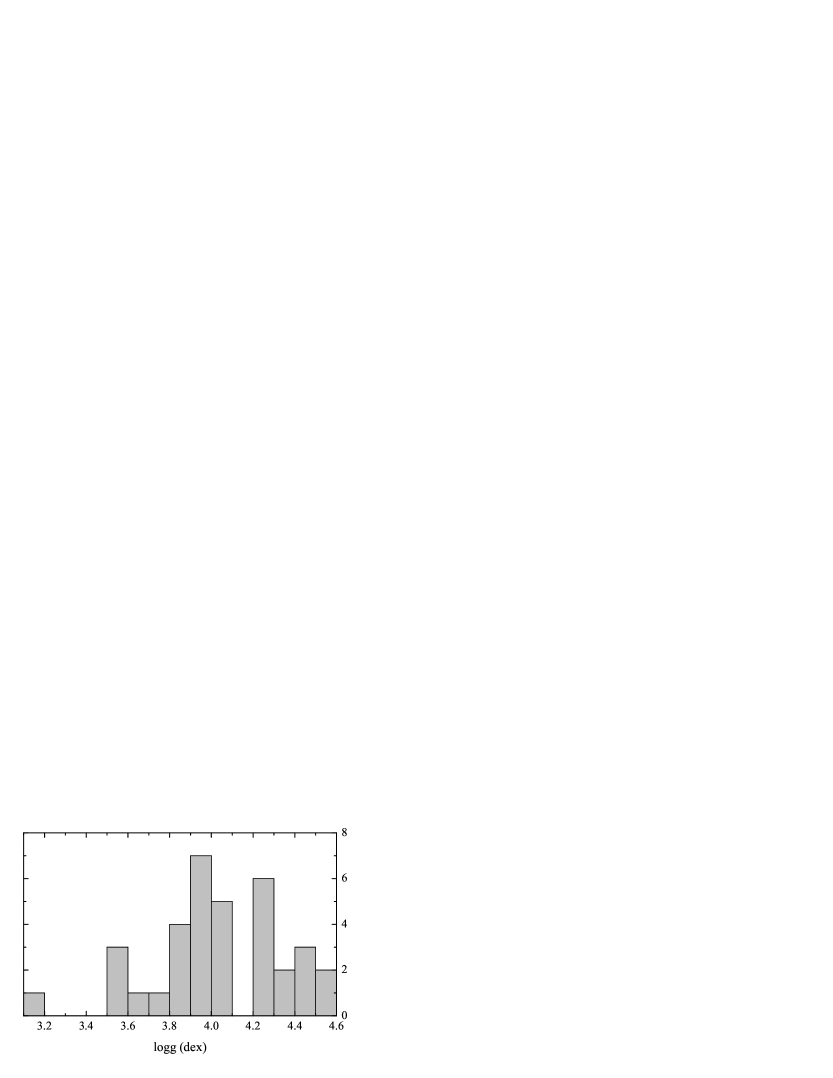
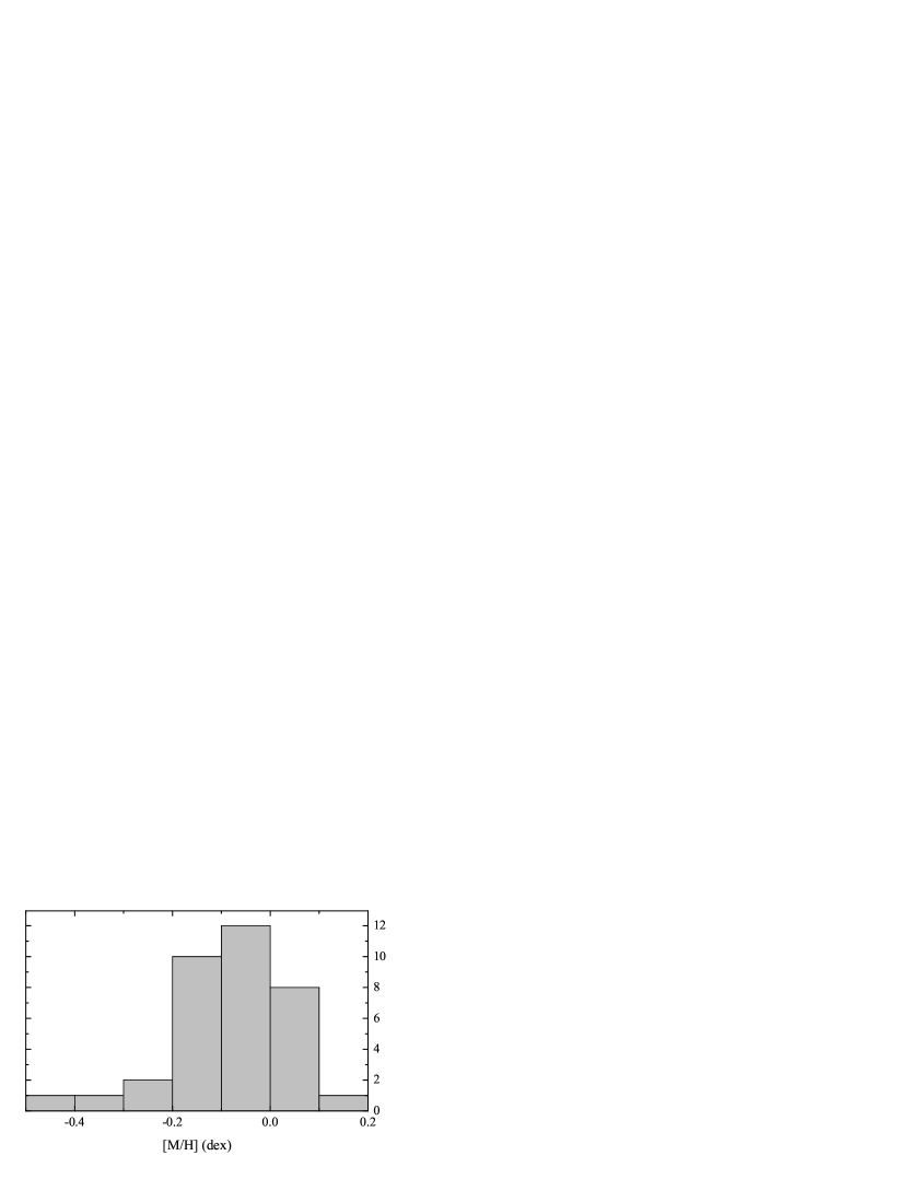
Figure 3: Distribution of effective temperatures (top left), surface gravities (top right), projected rotational velocities (bottom left), and metallicities (bottom right) of the sample targets.

For every star in our sample, we check for evidence of non-linear effects in the light curve by looking for low-order combination frequencies. We assume that any combination frequency should have lower amplitude than the parent frequencies, i.e. it should appear in a list which is sorted according to amplitude, below the frequency(ies) it is formed of. We allow up to three terms when computing the sum and/or difference combination frequencies, assuming that harmonics can enter the combination as well (e.g., f_i=2f₁+f₂-f₃ or f_i=f₁-3f₂+f₃). The frequency of interest is accepted to be a combination of the independent frequency if the difference between the combination and true values is less or equal to the Rayleigh limit. For example, the arbitrary frequency f_i is assumed to be a combination of the independent frequencies f₁ and f₂ when, e.g., $\mid$f${}_{\rm i}-$(2f₁+f₂)$\mid\leq$1/$T$.

Table B.1 summarizes the results of the frequency analysis for all 69 stars. The total time span of the observations and thus Rayleigh limit can vary from star to star and is indicated in the parenthesis following the star designation. The table lists the frequencies (both in d^-1 and $\mu$Hz) and corresponding amplitudes (in mmag), S/N, the corresponding lowest order combination, and the number of combinations that can be built of independent frequencies only. The latter number obviously needs more explanation. Each frequency in the list (except for the highest amplitude peak which is assumed to be independent), is first considered to be a possible combination term of the higher-amplitude parent frequencies. In the first step, we check for all possible combinations of the parent frequencies (all frequencies that have higher amplitudes than the one in question) capable of representing within the Rayleigh limit the frequency in question. Among the whole variety of the obtained combinations (the number of which will be the larger the lower is the amplitude of the frequency in question), we select those that involve the independent frequencies only. The total number of such combinations is given in the last column of Table B.1 designated “N”. A value of zero in this column means that the frequency of interest can only be represented as a combination of the frequencies which themselves are combinations of the independent peaks. In practice, this means that the frequencies with the number N=0 can only be represented as very high-order (typically, higher than 10) combinations, which is basically just a mathematical coincidence and has no physical meaning. The independent frequencies are highlighted in Table B.1 in boldface whereas their second- and third-order combinations are shown in italics and with the superscript “*”, respectively.

Pápics (2012a) investigated the problem of occurring combination frequencies in the light curves of $Kepler$ B-type stars. The author simulated thousands of light curves having similar but random power spectrum as the main-sequence SPBs. Pápics (2012a) concluded that one has to restrict to the low-order (up to the 3rd) combinations when interpreting the light curves as the higher-order combination peaks are likely mere coincidence than having any physical meaning. This is the reason why we consider only low-order (2nd and 3rd) combination peaks as having physical meaning while we are rather sceptical with respect to all other, higher-order combinations.

5 Spectroscopic analysis

As mentioned in Sect. 2, for half of the stars in our sample, we obtained high resolution (R=85 000) spectroscopic data. At least two spectra have been obtained for each star in order to check for possible RV variations due to binarity. Besides the binarity check, a collection of N independent spectra allows to increase S/N by roughly a factor of $\sqrt{N}$ by combining the single measurements and building an average spectrum. The gain in S/N is very important given that we aim for estimation of the fundamental stellar parameters like effective temperature $T_{\rm eff}$, surface gravity $\log{g}$, projected rotational velocity $v\sin{i}$, and metallicity [M/H].

As for the second half of the sample stars, their observations are planned for the summer next year when the $Kepler$ field is best visible on La Palma, Canary Islands. Besides that, we also plan more extensive spectroscopic monitoring of the stars for which more than just a couple of measurements would be essential (e.g., spectroscopic binaries for which a precise orbital solution and possibly decomposed spectra in the case of double-lined binaries (SB2) can be derived given that good orbital phase coverage is provided). In the following, we describe the results of our spectrum analysis of 36 of the sample stars and compare the spectroscopic classification with the one based on the method by Debosscher et al. (2011).

5.1 Fundamental parameters and position in the HR diagram

For estimation of the fundamental parameters of the stars, we use the GSSP code (Tkachenko et al. 2012; Lehmann et al. 2011). The code relies on a comparison between observed and synthetic spectra computed in a grid of $T_{\rm eff}$, $\log{g}$, $v\sin{i}$, [M/H], and microturbulent velocity $\xi$, and finds the optimum values of these parameters from a minimum in $\chi^{2}$. Besides that, individual abundances of different chemical species can be adjusted in the second step assuming a stellar atmosphere model of a certain global metallicity. The grid of atmosphere models has been computed using the most recent version of the LLmodels code (Shulyak et al. 2004) in [–0.8, +0.8] dex, [4 500, 22 000] K, and [2.5, 5.0] dex range for metallicity, effective temperature, and surface gravity, respectively (Tkachenko et al. 2012). Synthetic spectra are computed using the SynthV code (Tsymbal 1996) which allows to compute the spectra based on individual elemental abundances, to take vertical stratification of a chemical element and/or microturbulent velocity into account.

The errors of measurement (1$\sigma$ confidence level) are calculated from the $\chi^{2}$ statistics using the projections of the hypersurface of the $\chi^{2}$ from all grid points of all parameters onto the parameter in question. In this way, the estimated error bars include any possible model-inherent correlations between the parameters. Possible imperfections of the model like incorrect atomic data, non-LTE effects, or continuum normalization are not taken into account. In a recent study by Molenda-Żakowicz et al. (2013) the use of different methods and codes to derive atmospheric parameters for F, G, K, and M-type stars is compared, and led the authors to conclude that the realistic accuracy in the determination of atmospheric parameters for these types of stars is $\pm$ 150 K in $T_{\rm eff}$, $\pm$ 0.15 dex in [Fe/H], and 0.3 dex in $\log{g}$, even though error calculations for individual programs might result in smaller errors. Hence, we are aware of a possible underestimation of errors in Table 4.

Figure 4: Location of 36 stars (see Table 4) and the $\gamma$ Dor and $\delta$ Sct (solid lines) theoretical instability strips (Dupret et al. 2005) in the HR diagram. Dashed thin and thick lines represent the $\gamma$ Dor instability regions computed with $\alpha=2.0$ and 1.5, respectively. Open circles refer to the hybrid pulsators.

Given the rather low S/N of our spectra (typically, below 80 for the average spectrum), we decided to fix the microturbulent velocity $\xi$ to the standard value of 2 km s^-1 and optimise the global metallicity (which is a scaling of all chemical elements heavier than hydrogen and helium by the same factor) instead of evaluating individual abundances of chemical elements. Table 4 summarizes the results of the spectroscopic analyses of the 36 stars in our sample listing the KIC-number, $T_{\rm eff}$, $\log{g}$, $v\sin{i}$, and [M/H] values, as well as the number of individual spectra used for building the average spectrum.

Figure 3 shows distributions of the four fundamental parameters of the sample stars. The majority of the targets (about 66 %) have effective temperatures in the range between 6 900 and 7 200 K though a few objects show slightly higher/lower ($\pm$ 200 K) temperature values. The distribution of the surface gravities suggests that all but one stars are luminosity class IV-V sub-giant or main-sequence stars, which together with the above mentioned temperature regime, perfectly fits the classical definition of the $\gamma$ Dor stars group (see, e.g. Kaye et al. 1999; Aerts et al. 2010). The largest majority of the targets, within the error of measurements, show solar metallicities though a couple of stars exhibit slightly depleted overall chemical composition compared to the Sun. Our sample is dominated by slowly ($v\sin{i}$$<$30 km s^-1) and moderately (30$<$$v\sin{i}$$<$100 km s^-1) rotating stars, only seven objects have $v\sin{i}$ values above 100 km s^-1.

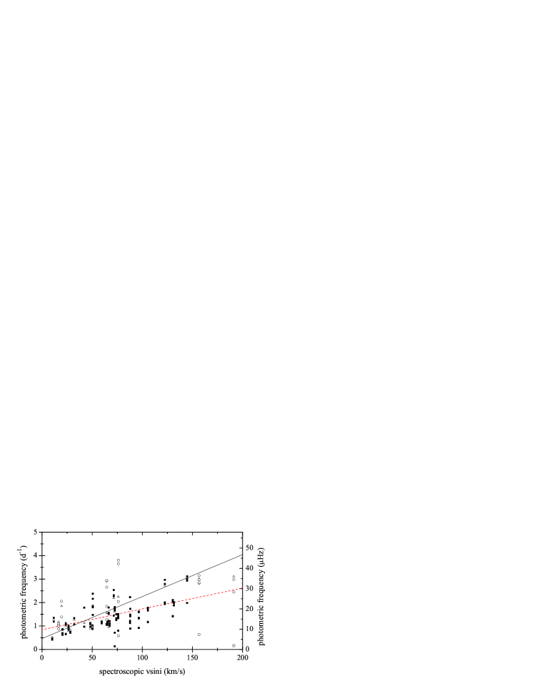
Figure 5: $v\sin{i}$ versus independent frequencies for the sample stars. Open triangles refer to the dominant oscillation mode for each star, the two other symbols represent all other independent frequencies. Filled boxes and open circles refer to $\gamma$ Dor and hybrid pulsators, respectively. The solid black line shows linear fit to all data points (there are three frequencies between 18 (208.26) and 21 (242.97) d^-1 ($\mu$Hz) in the $\delta$ Sct domain), the red dashed line represents a linear fit to the frequencies in the $\gamma$ Dor range after removing the $\delta$ Sct frequencies.

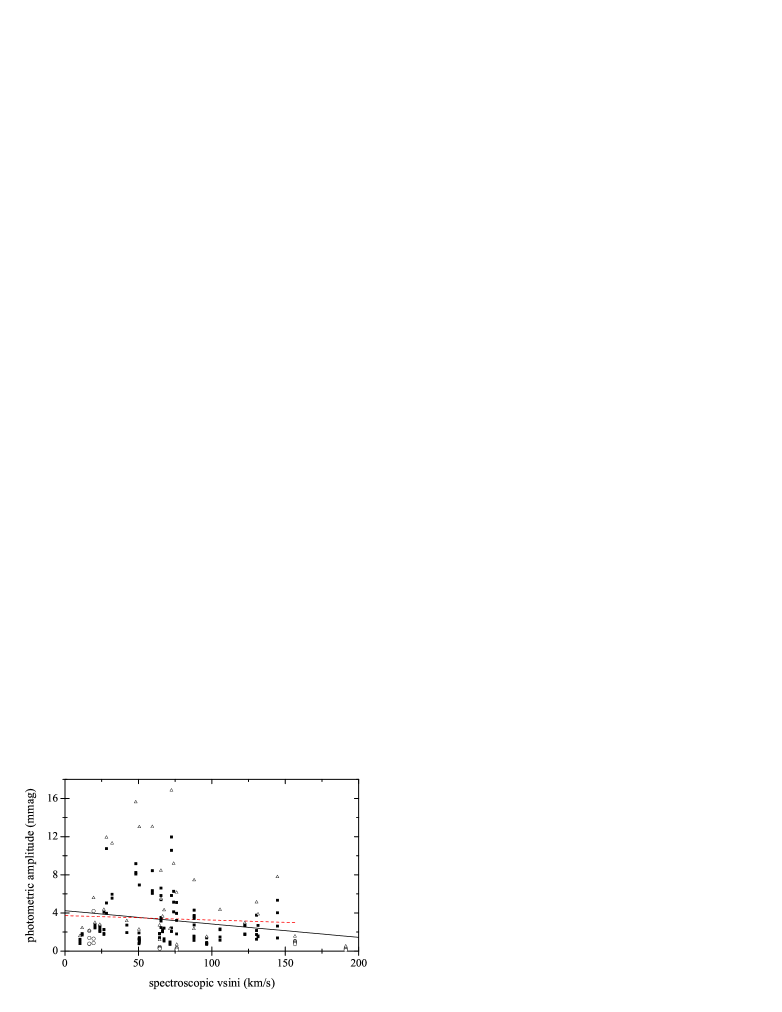
Figure 6: Same as Fig. 5 but for the amplitudes. The solid black line shows a linear fit to all data points, the red dashed line represents a linear fit after removing two stars with $v\sin{i}$$>$150 km s^-1 from the sample.

The derived values of $T_{\rm eff}$ and $\log{g}$ allow us to place the stars into the log (L/L_⊙)–log $T_{\rm eff}$ diagram and classify them by evaluating their positions relative to the $\gamma$ Dor and $\delta$ Sct theoretical instability strips. The luminosity of each star has been estimated from an interpolation in the tables by Schmidt-Kaler (1982) using our spectroscopically derived $T_{\rm eff}$ and $\log{g}$. The errors in luminosity were evaluated by taking the errors of both $T_{\rm eff}$ and $\log{g}$ into account. However, we base our spectroscopic classification mainly on the position of the stars according to the derived temperatures as the luminosity errors can still be underestimated due to the uncertainties in the empirical relations.

Figure 4 shows the position of the stars in the HR diagram together with the $\gamma$ Dor and $\delta$ Sct theoretical instability strips. The latter are based on Dupret et al. (2005, Figures 2 and 9). The edges of the $\delta$ Sct instability region have been computed for the fundamental mode and a mixing-length parameter of $\alpha=1.8$ (solid lines). The borders of the $\gamma$ Dor instability regions computed with $\alpha=2.0$ and 1.5 are shown by dashed thin and thick lines, respectively. All stars but one are nicely clustering in the region of the HR diagram where the $\gamma$ Dor-type g-mode pulsations are expected to be excited in stellar interiors. KIC 08378079 is the only “outlier” located the top left (towards higher temperatures and more luminous objects) of the $\gamma$ Dor instability region in the diagram (cf. Figure 4). Given that our average spectrum is of very low S/N and thus the error bars in both temperature and luminosity are large for this faint ($V=12.5$) star, it can safely be considered as a $\gamma$ Dor-type variable from our spectroscopic values of $T_{\rm eff}$ and $\log{g}$.

As an overall conclusion, our spectroscopic classification perfectly agrees and thus confirms the photometric one based on the information derived from the $Kepler$ light curves only (cf. Sect. 3). A second important conclusion for future asteroseismic modelling is that most stars are slow to moderate rotators. Of course, the estimated value of the projected rotational velocity is not a measure of the true rotational period of a star but allows to put some constraints (lower limit) on the stellar rotation frequency.

Figure 7: Frequency of the dominant mode as a function of $v\sin{i}$ for $\delta$ Sct stars from the catalogues of Rodríguez et al. (2000, top) and Uytterhoeven et al. (2011, bottom). The solid line represents a linear function fit to the shown data points. Detailed information on individual stars is provided in Table A.1.

We also checked for a possible correlation between the spectroscopically derived value of $v\sin{i}$ and photometric frequencies of the independent pulsation modes for each star. The distribution is illustrated in Figure 5. There is a clear trend in the $v\sin{i}$-frequency diagram implying that the independent mode frequencies are higher for the larger $v\sin{i}$. The correlation becomes even stronger if we include the three frequencies from the $\delta$ Sct domain that we detected for two of the shown stars (solid, black line to be compared with the dashed, red line in Figure 5). For completeness, in Figure 6, we also present the $v\sin{i}$-amplitude distribution for the sample stars. Though a negative trend shows up when fitting all the data points linearly (solid line), it is almost gone when the two stars with $v\sin{i}$$>$150 km s^-1 are removed (dashed line). Thus, we conclude that the $v\sin{i}$-amplitude correlation presented here is at best weak and is not a characteristic of $\gamma$ Dor stars.

To check whether a similar $v\sin{i}$-frequency correlation is also characteristic of $\delta$ Sct stars, we used the data from the catalogues of Rodríguez et al. (2000, hereafter called R2000) and Uytterhoeven et al. (2011). All stars for which $v\sin{i}$ measurements are available were selected, resulting in 189 and 16 objects extracted from R2000 and Uytterhoeven et al. (2011), respectively. The full list of the retrieved objects is given in Table A.1. We are also aware of the two recent extensive studies by Balona & Dziembowski (2011) and Chang et al. (2013) focusing on the $\delta$ Sct stars but these authors do not present $v\sin{i}$-frequency correlations in their papers. The $v\sin{i}$-frequency distributions obtained based on the data from R2000 and Uytterhoeven et al. (2011) are illustrated in Figure 7. In both cases, linear fits (solid lines in both panels) show a negative trend, though with different slopes: it is steeper for the Uytterhoeven et al. (2011) data than for those from R2000. However, the reliability of the correlation shown in the bottom panel of Figure 7 is not convincing because of too few objects that could be retrieved from the sample of Uytterhoeven et al. (2011). Comparison of the R2000 distribution (cf. Figure 7, top panel) with the one we obtained for the $\gamma$ Dor stars in this paper (cf. Figure 5), reveals opposite behaviour: for the $\gamma$ Dor stars, the frequencies of oscillation modes are found to increase as the $v\sin{i}$ increases whereas they decrease or, at most, remain constant for the $\delta$ Sct stars.

From Figure 5, it is clear that not only the dominant mode frequencies (open triangles) but also all the other independent frequencies (filled boxes and open circles) show a correlation with $v\sin{i}$. If the correlation was due to rotational modulation, one would expect only the dominant, rotation frequency to show dependence on $v\sin{i}$. Since we observe several independent frequencies for each star and they all show similar behaviour with respect to $v\sin{i}$ (cf. Figure 5), we conclude that the observed correlation is due to stellar pulsations rather than rotational modulation. Moreover, besides the above mentioned correlation for the rotation frequency, one would also expect the rotational modulation to show up with series of harmonics of that frequency (see e.g., Thoul et al. 2013). We thus checked how many harmonics in total (including those of combination frequencies) per star could be detected and present the distribution in Figure 8 (top). Though there is a clear peak at three harmonics per star, the distribution is rather random, revealing stars showing up to a couple of dozens of harmonics in their light curves. The majority of these detections are harmonics of (very low-amplitude) combination frequencies which is likely to be just a mathematical coincidence rather than having any physical meaning (see Pápics 2012a). Indeed, none of the stars show a series of harmonics but rather single peaks for combination frequencies. We thus reconsidered our distribution including only harmonics of the independent frequencies now (see Figure 8, bottom). There is a clear peak at three harmonics per star and the largest number of the detected harmonics per object decreased from the previous 29 to the present 9. A careful look at the independent frequencies and their harmonics showed that the latter are homogeneously distributed among all independent frequencies and there is no star showing a long series of harmonics of a single independent frequency as one would expect for rotational modulation.

Figure 8: Distributions of the total number of the detected harmonics (top) and those formed of independent frequencies only (bottom).

6 Discussion and conclusions

Non-uniform period spacings of gravity pulsation modes is a powerful tool for diagnostics of the properties of the inner core and its surrounding layers. We aim for the application of the methodology described by Miglio et al. (2008) and Bouabid et al. (2013) (for the first practical application, see Degroote et al. 2010) to $\gamma$ Dor-type pulsating stars. This paper is the first step towards this goal.

Based on an automated supervised classification method (Debosscher et al. 2011) applied to the entire $Kepler$ Q1 dataset of about 150 000 high-quality light curves, we compiled a sample of 69 $\gamma$ Dor candidate stars. We presented the results of frequency analyses of the $Kepler$ light curves for all stars in our sample. For each star, we checked the results for evidence of non-linear effects in the light curve by looking for low-order combination frequencies. All our stars show at least several second-order and third-order combination frequencies (including harmonics) suggesting that non-linear effects are common for $\gamma$ Dor-type pulsating stars.

From the $Kepler$ light curve analysis, we identified 45 $\gamma$ Dor stars, 14 hybrid pulsators, and 10 stars marked as “possible $\gamma$ Dor/$\delta$ Sct hybrids” and showing low amplitude, high-order (typically, higher than 6-8) combinations in the p-mode regime of the Fourier spectrum. A more detailed study of the amplitude spectra would be needed for these ten stars to classify them correctly. According to the highest amplitude frequency distribution (cf. Figure 9), the $\gamma$ Dor-type g-mode pulsations dominate our sample and there is only one star, KIC 06778063, where the peak in the p-mode regime is the dominant one in the data.

Additionally, high-resolution spectroscopic data have been obtained for half of our stars with the HERMES spectrograph (Raskin et al. 2011) attached to the 1.2-m Mercator telescope. All 36 stars for which spectra have been acquired fall into the $\gamma$ Dor instability region confirming the photometric classification as either $\gamma$ Dor- or of $\gamma$ Dor/$\delta$ Sct hybrid-type pulsating stars. The effective temperatures are distributed within a narrow window of 700 K, the surface gravities distribution suggests luminosity class IV-V sub-giant or main-sequence stars. Hence, the applied method of photometric classification as described in Debosscher et al. (2011), proves to be very robust.

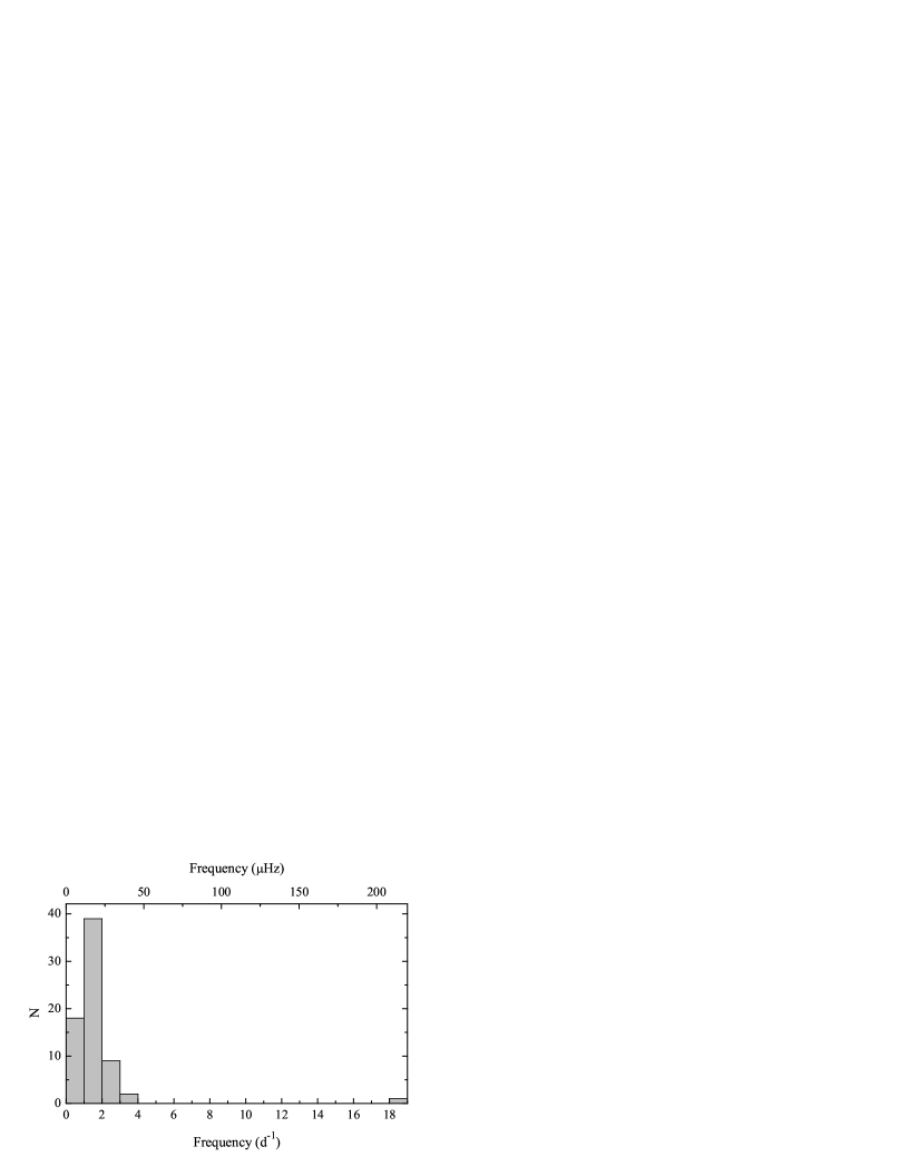
Figure 9: Distribution of the highest amplitude frequency detected in the Fourier spectra of the sample stars.

Uytterhoeven et al. (2011) presented a characterization of a large sample of A- to F-type stars based on $Kepler$ photometry and, where available, ground-based spectroscopy. Among the stars showing $\gamma$ Dor, $\delta$ Sct, or both types of pulsations in their light curves, the authors identified about 36% as hybrid pulsators. In our case, this fraction is about 35% if we consider 10 “possible $\gamma$ Dor/$\delta$ Sct hybrids” as being indeed hybrid pulsators and about 20% if we exclude them. An extrapolation of the results obtained by Uytterhoeven et al. (2011) for a sub-sample of 41 targets to the entire sample, led the authors to the conclusion that many of $\gamma$ Dor and $\delta$ Sct pulsators are moderate (40$<$$v\sin{i}$$<$90 km s^-1) to fast ($v\sin{i}$$>$90 km s^-1) rotators. Our sample consists of mainly slow to moderate rotators with the $v\sin{i}$ distribution peaking at the value of 65 km s^-1 (cf. Figure 3, bottom left). The major conclusion that Uytterhoeven et al. (2011) made concerning $\gamma$ Dor and $\delta$ Sct theoretical instability strips was that they have to be refined as the stars with characteristic type of pulsations seem to exist beyond the respective instability regions. The studies preformed by Grigahcène et al. (2010); Tkachenko et al. (2012, 2013) led to similar conclusions. Also Hareter (2012), who studied a large number of the CoRoT light curves, found that $\gamma$ Dor stars mainly cluster at the red edge of the $\delta$ Sct instability strip, with a significant fraction of them having cooler temperatures however, whereas $\delta$ Sct-$\gamma$ Dor hybrid pulsators fill the whole $\delta$ Sct instability region with a few stars being beyond its blue edge. The author also concludes that, from the position of the studied objects in the HR diagram, there is no close relation between $\gamma$ Dor stars and hybrid pulsators. In this paper, we found that all stars for which fundamental parameters could be measured from spectroscopic data, reside in the expected range of the HR diagram, clustering inside the theoretical $\gamma$ Dor instability region. Our results are based on different i.e., much stricter, selection criteria than those applied in the above mention papers, i.e. the morphology of the light curves in combination with a spectroscopic $T_{\rm eff}$ determination rather than a poor $T_{\rm eff}$ estimate or colour index alone. This implies that our sample is much “cleaner” and not contaminated by stars with other causes of variability than pulsations.

Balona et al. (2011) suggested that the pulsation and rotation periods must be closely related. Given that in Uytterhoeven et al. (2011) $v\sin{i}$ values were obtained for a very limited number of stars, the authors did not look for any correlations between $v\sin{i}$ and pulsation period/frequency. In our case, we have found a clear correlation between the spectroscopically derived $v\sin{i}$ and the photometric frequencies of the independent pulsation modes (cf. Figure 5) in a sense that the modes have higher frequencies the faster is the rotation. This correlation is not caused by rotational modulation of the analysed stars but is valid for the $\gamma$ Dor g-mode stellar oscillations. These findings are in perfect agreement with the results of the recent theoretical work by Bouabid et al. (2013), who showed that the rotation shifts the g-mode frequencies to higher values in the frequency spectrum of a pulsating star, filling the gap between the $\delta$ Sct-type p- and $\gamma$ Dor-type g-modes. Comparison with the $\delta$ Sct stars reveals that they behave in the opposite way, namely they show decreasing frequency as the $v\sin{i}$ increases. We also checked for a $v\sin{i}$-amplitude correlation for our $\gamma$ Dor stars but did not get any convincing results.

Compared to the study by Uytterhoeven et al. (2011) where a large sample of 750 A- to F-type stars has been analysed and of which about 21% were found not to belong the class of $\gamma$ Dor or $\delta$ Sct nor to the hybrid pulsators, 12% were identified as binary or multiple star systems, and many objects were found to be constant stars, our sample is much more homogeneous and does not include “bias”, i.e., all selected stars are multiperiodic pulsators. Compared to the sample of CoRoT stars compiled by Hareter (2012), nearly continuous $Kepler$ observations spread over several years offer an order of magnitude higher frequency resolution which allows to resolve the frequency spectrum and makes the detection of frequency and period spacings possible. Hence, our sample selection and frequency analysis offer a good starting point for seismic modelling of $\gamma$ Dor stars.

In follow-up papers, we plan to present the detailed frequency analysis results for all individual stars as well as a spectroscopic analysis of the fainter stars in the sample, in addition to seismic modelling based on the observational results.