A dynamical programming approach for controlling the directed abelian Dhar-Ramaswamy model

Abstract

A dynamical programming approach is used to deal with the problem of controlling the directed abelian Dhar-Ramaswamy model on two-dimensional square lattice. Two strategies are considered to obtain explicit results to this task. First, the optimal solution of the problem is characterized by the solution of the Bellman equation obtained by numerical algorithms. Second, the solution is used as a benchmark to value how far from the optimum other heuristics that can be applied to larger systems are. This approach is the first attempt on the direction of schemes for controlling self-organized criticality that are based on optimization principles that consider explicitly a tradeoff between the size of the avalanches and the cost of intervention.

1 Introduction

Self-organized criticality (SOC) is a characteristic of systems that are driven by a slowly acting external force and organize themselves through energy dissipating avalanches of all sizes. Although SOC models were first proposed to explain the origin of the $1/f$ noise, it is recognized that it can be used to explain a large class of systems such as earthquakes [sch91], evolutionary bursts [baksne93], forest fires [drosch92], rice piles [fre96], financial markets [bar06], and so on.

Recently we have raised the issue that, for some critical organized systems, the size of the largest avalanches can be reduced by a control intervention heuristics [cajand10]. That was just a first effort to investigate if and how the damaging energy dissipative bursts in SOC systems could be controlled. Although such systems organize themselves without external intervention, this reorganization in a lower level of energy is very costly for society, since it depends on avalanches of all sizes. Examples of these events of dissipation of energy in nature and society are avalanches that arise in snow hills, bubbles that explode in financial markets and earthquakes. Although it is not possible to intervene in events such as earthquakes, in some sense we can intervene in the process that generates large snow avalanches and the explosion of stock bubbles. In the former case, small avalanches can be triggered in order to avoid larger ones [mccsch93]. In the later case, central banks can in some sense enforce a monetary policy that can avoid the rising of large bubbles [greenspan08]. Regarding this aspect, it is not the purpose of this work to defend this kind of procedure, but we surely think that it deserves to be studied. Our first investigation  [cajand10], was based on a replica model of the region of the system to be controlled, a control scheme was designed to externally trigger small size avalanches in order to avoid larger ones. Although we have shown that this principle works for sandpiles in two-dimensional lattices [cajand10], we have no information about how far from the optimal choice these heuristics are. To fill this gap we resume our investigation with a rather different approach: we develop a dynamical programming (DP) approach to control the directed abelian Dhar-Ramaswamy (DADR) model in a two dimensional lattice. Due to the huge number of possible states that come to play in DP approaches, any feasible investigation must be restricted to systems of much smaller size than those one usually considers when performing numerical integration of the systems. Nevertheless, we can use this approach to characterize optimally the problem of controlling SOC systems, as well as to explore the efficiency of other heuristics built without any kind of optimization law and as a basis for approximate optimization principles such as the ones presented in [bertsi96].

It is worth mentioning that recent literature has used optimization principles to understand the structure and dynamics of several complex systems. In [rodrin92, caj05, jacrog05, mottor07, carior08], it was shown that complex networks may arise from optimization principles. Further, analyzes of optimal navigation in complex networks [caj09, caj10] have shown that a walker that minimizes the cost of walking overlaps the random walker and the directed walker behaviors. In [cajmal08, ast08] optimization has been used to study the complex human dynamics of task execution. Moreover, reinforcement learning has been used to explore the problem of learning paths in complex networks [cajand09].

2 The DP approach for controlling the DADR model

The DADR model [dha89] is built on a two-dimensional square lattice of $L\times L$ sites $(i,j)$, $i,j=1,\cdots,L$. Each site stores a certain amount $z_{ij}$ of mass units. At each time step, the system is driven by two update rules: (a) Addition rule: a mass unit is added to a randomly selected site $(k,\ell)$, so that $z_{k\ell}\rightarrow z_{k\ell}+1$. (b) Toppling rule: if $z_{ij}>z_{c}=1$, then $z_{ij}\rightarrow z_{ij}-2$, $z_{i+1,j-1}\rightarrow z_{i+1,j-1}+1$ and $z_{i+1,j+1}\rightarrow z_{i+1,j+1}+1$. The model is usually represented after performing a $5\pi/4$ rotation of the standard square lattice, in such a way the site $(i+1,j+1)$ lies just below the site $(i,j)$, and the $\mathbf{x}$ and $\mathbf{y}$ directions are at $5\pi/4$ and $7\pi/4$ angles with the horizontal axis. Therefore, if deposition occurs in site $(i,j)$, the only sites that may be affected are those located on the lines $i+\ell,\ell\geq 1$.

Let $\Gamma$ be the finite set of stable states (configurations) in the phase space of the DADR model, and $N_{\Gamma}$ the number of elements of $\Gamma$. As in any DP study, it is necessary to identify the different actions (or policies) that can be taken when the system is in any of these states. So let us note such one policy as $\pi=[u(1),\cdots,u(N_{\Gamma})]$, where $u(i)\in U$ refers to the specific control action that $\pi$ undertakes when the system is in the state $i$. $U$ represents the set of admissible controls, i.e. those control actions that do not violate the system dynamics. Note that the number of elements in the set $\Pi$ of all admissible policies $\pi$ increases faster than combinatorial when the system size increases. Indeed, this number depends both on $N_{\Gamma}$ and on the number of possible control actions for each state $i$.

To control the avalanches sizes in our approach, it is important to consider that events occur according to an ordered sequence, as discussed in  [cajand10]. If $t$ is a discrete variable $t=n\Delta t$, and the DADR model is in a given “stable” state $x_{t}$ we assume that the following events take place within the time step $\Delta t$. The control scheme triggers (or not) one avalanche in a specific site $(i,j)$ of the lattice. If this occurs, the avalanche starts by emptying the site $(i,j)$, what amounts to topple the single unit mass with $50\%$ of probability to the site $(i+1,j-1)$ or to the site $(i+1,j+1)$. This control induced toppling may lead to further toppling until the system reaches a new stable state $x_{t}^{c}$ due to the control intervention $u(x_{t})$. After this induced avalanche, which is absent if the used policy indicates to take no action, the usual deposition process of the model takes place and the system evolves from either $x_{t}$ or $x_{t}^{c}$ to a new state $x_{t+1}$. For this process, we only care that control intervention comes before the deposition process, and that both relaxations occur within the same time step $\Delta t$.

However, differently from [cajand10], we assume here that there is only possible at most one control intervention per time step, and the intervention decision is made according to a dynamic programming approach.

For instance, if $L=2$, then $N_{\Gamma}=2^{L^{2}}=2^{2^{2}}=16$. One possible state of $\Gamma$ is

$$x=\left[\begin{array}[]{cc}0&1\\ 1&0\\ \end{array}\right].$$ (1)

Please note that, for the purpose of keeping a simple diagram, we did not perform the rotation used for the representation of the system described before. In such matrix-like notation, the toppling process makes the grain move either one column to the right or one line downwards. Assume $x$ to be $x_{t}$. In this state, we have three admissible controls, namely the one that triggers no avalanche, and those that trigger an avalanche in the sites $(1,2)$ and $(2,1)$, respectively. If there is no intervention, the intermediate state $x_{c}(t)=x(t)$. If an avalanche is triggered in the site $(1,2)$, the system goes to $x_{t}^{c}$ which, with equal probabilities, is one of the states

$$\left[\begin{array}[]{cc}0&0\\ 1&1\\ \end{array}\right],\left[\begin{array}[]{cc}0&0\\ 1&0\\ \end{array}\right].$$

(If the site $(2,1)$ had been chosen, the situation would be quite similar but, for the sake of brevity, we will not consider this choice here.) In order to differ one state from the other, we call the one in the left as $x_{t}^{c,L}$ and the one in the right as $x_{t}^{c,R}$, making reference to the side followed by the controlled avalanche. Thus, after the deposition process, the system can have suffered a transition to one of the following states, in the case of $x_{t}^{c,L}$,

$$\left[\begin{array}[]{cc}1&0\\ 1&1\\ \end{array}\right],\left[\begin{array}[]{cc}0&1\\ 1&1\\ \end{array}\right],\left[\begin{array}[]{cc}0&0\\ 0&0\\ \end{array}\right],\left[\begin{array}[]{cc}0&0\\ 1&0\\ \end{array}\right].$$

or to one of the possible states, if $x_{t}^{c,R}$ was taken:

$$\left[\begin{array}[]{cc}1&0\\ 1&0\\ \end{array}\right],\left[\begin{array}[]{cc}0&1\\ 1&0\\ \end{array}\right],\left[\begin{array}[]{cc}0&0\\ 0&1\\ \end{array}\right],\left[\begin{array}[]{cc}0&0\\ 1&1\\ \end{array}\right].$$

Therefore, with equal probabilities, the state $x_{t+1}$ will be represented by one of these eight states. One also must note that, associated with the control intervention and the deposition process, we have respectively two classes of avalanches: controlled avalanches, that are triggered by the control scheme in state $x_{t}$ with sizes $s_{c,x_{t}\,x_{t}^{c,L}}$ or $s_{c,x_{t}\,x_{t}^{c,R}}$ depending on the side that the controlled avalanche followed; and uncontrolled avalanches with sizes $s_{u,x_{t}^{c,L}\,x_{t+1}}$ or $s_{u,x_{t}^{c,R}\,x_{t+1}}$ that happen when the system goes from state $x_{t}^{c,L}$ or $x_{t}^{c,R}$ to state $x_{t+1}$ due to the deposition process.

Following the DP approach, we assume that the control scheme makes the decision of triggering an avalanche in one site of the system or doing nothing in a given state $x$ based on the minimization of the cost function

$$J(x)=\min_{\pi\in\Pi}E^{\pi}\left[\sum_{t=0}^{\infty}\gamma^{t}g(x_{t},u(x_{t}))|x\right]$$ (2)

where the expectation $E^{\pi}[\cdot|x]$ is conditional on the policy $\pi$ and the state $x$. The cost per stage $g(\cdot,\cdot)$ is given by

$$g(x_{t},u(x_{t}))=\sum_{x_{t+1}}p_{x_{t}x_{t+1}}(u)\overline{g}(x_{t},u(x_{t}),x_{t+1}),$$ (3)

where $u(x_{t})$ is the control intervention in state $x_{t}$, $\overline{g}(x_{t},u(x_{t}),x_{t+1})$ is the cost of using the control $u$ at state $x_{t}$ and moving to state $x_{t+1}$, $p_{x_{t}x_{t+1}}(u)$ is the transition probability from state $x_{t}$ to state $x_{t+1}$ using the control $u$ at state $x_{t}$. In the general expression (3), the function form of $\overline{g}$ has not yet made explicit. In this work, we assume a simple particular form for $\overline{g}$ that depends only on two parameters and a functional dependence on the avalanche size $s$. Therefore, we write

$$g(x_{t},u(x_{t}))=C_{I}I(x_{t})$$

$$+\frac{1}{2}[C_{A}h(s_{c,x_{t}\,x_{t}^{c,L}})+\sum_{x_{t+1}}p_{x_{t}^{c,L}x_{t+1}}C_{A}h(s_{u,x_{t}^{c,L}\,x_{t+1}})]$$

$$+\frac{1}{2}[C_{A}h(s_{c,x_{t}\,x_{t}^{c,R}})+\sum_{x_{t+1}}p_{x_{t}^{c,R}x_{t+1}}C_{A}h(s_{u,x_{t}^{c,R}\,x_{t+1}})],$$

where $p_{x_{t}^{c,L}x_{t+1}}$ (or $p_{x_{t}^{c,R}x_{t+1}}$) is the probability of transition from $x_{t}^{c,L}$ (or $x_{t}^{c,R}$) to $x_{t+1}$. One must also note that, while $p_{x_{t}x_{t+1}}(u)$ indicates explicitly that the probability of the transition from state $x_{t}$ to state $x_{t+1}$ depends on the choice of the control $u$ at state $x_{t}$, $p_{x_{t}^{c,L}x_{t+1}}$ (or $p_{x_{t}^{c,R}x_{t+1}}$) does not present this dependence. $I(x_{t})$ is an indicator function that assumes the value 1, when there is an intervention in state $x_{t}$, and 0 otherwise. Finally, the two parameters $C_{I}$ and $C_{A}$ represent the fixed cost associated with one intervention and avalanche size. For the sake of simplicity, we assume here that $h(s)=s^{2}$, i.e., we penalize larger avalanches in a power law with exponent equal to 2.

The term $\gamma^{t}$ in (2) weights differently the influence of the present and future costs in the decision process. Although a realistic optimization process must take into account the intervention cost, it could be expected that avalanches at a given time step and those in the next future should have approximately the same weight in the decision process, what amounts to take the discount factor $\gamma=1$. We call the attention that this simple choice leads to a technical difficult, namely, we can not ensure that this problem has a solution that does not depend on the kind of the controlled Markov process. In such situations, the method used to solve the problem may depend on the type of the controlled Markov chain that we are dealing with and may be difficult to find by simple algorithms [put05]. However, due to the Banach Fixed Theorem [put05], this difficult can be circumvented if we consider $\gamma\rightarrow 1_{-}$. Finally we should also note that the choice $\gamma=1$ is somewhat unrealistic as it does not consider the cost of the money over time.

It is easy to show that the solution of problem (2) is given by the Bellman equation [bel57]

$$J(x)=\min_{u\in U(x)}\left[g(x,u)+\sum_{x^{\prime}}p_{xx^{\prime}}(u)\gamma J(x^{\prime})\right].$$ (5)

In the rest of this paper, we discuss the solution of problem (2) using numerical solutions of the Bellman equation (5) found by means of the value iteration algorithm [put05].

3 Results

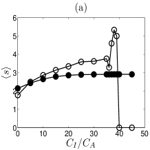
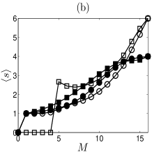
Figure 1: (a) The avalanche average size for several values of the ratio $C_{I}/C_{A}$: controlled avalanches (hollow circles) and uncontrolled avalanches (solid circles). (b) The average size of the avalanches for several values of the mass of the state. While solid symbols represent uncontrolled avalanches, hollow symbols represent controlled avalanches: $C_{I}/C_{A}=0$ (circles) and $C_{I}/C_{A}=10$ (squares).

The main difficulty associated with DP approach is the rapid increase of $N_{\Gamma}$ which, for the current study, behaves like $2^{L^{2}}$. For practical purposes, it becomes impossible to study numerically a system larger than $L=4$. As already discussed, the size of such system in much smaller than lattice sizes actually used to compute the time evolution of the model. However, we will show that this approach can be used to characterize the optimal solution of the problem and be used as a benchmark to validate other solutions based on ad-hoc chosen heuristics.

For all simulations of DADR’s model reported in this paper, the corresponding solution of Eq. (5) was obtained for $L=4$ and $\gamma=0.999$. For this value of $L$, $N_{\Gamma}=65536$, the largest avalanche that can take place in such system is of size $s=16$, the minimal and maximal amount of mass $M$ kept in the system are, respectively, $M=0$ and $M=16$. For the next lattice size $L=5$, solving (5) requires to find the minimum of $J(x)$ by taking into account all $2^{25}\sim 3.2\times 10^{7}$ states for this lattice size.

At a given time $t$, the number of admissible controls depends on the state $x$. For instance, while in the unique state of the system with mass 0, there is only one control, which is to do nothing, in the unique state of the system with mass 16, there are 17 admissible controls.

Figure 1(a) shows the effect of the the cost $C_{A}$ and $C_{I}$ in the solution of the problem presenting the average controlled and uncontrolled avalanches $\langle s\rangle$ for different values of $C_{I}/C_{A}$. It is shown that, when the cost of making interventions becomes high, the control scheme waits until the system has stored a larger amount of mass $M$ to make interventions. This causes also the size of the uncontrolled avalanches to increase. For a given threshold value $(C_{I}/C_{A})_{T}\sim 40$, intervention cost becomes so large that the optimal solution corresponds to not intervene in the system anymore. Correspondingly, when $C_{I}/C_{A}$ is close to $(C_{I}/C_{A})_{T}$, the number of interventions decreases exponentially (not shown). Figure 1a also shows that, for $C_{I}/C_{A}>(C_{I}/C_{A})_{T}$, only avalanches produced by the system dynamics are observed.

It turns out that $M$ is an interesting metric that can be used to order the states of the system in terms of danger of larger avalanches. Figure 1(b) shows the average size of avalanches for several values of $M$ for the ratios $C_{I}/C_{A}=0$ and $C_{I}/C_{A}=10$. This figure shows the effect of the increasing the ratio $C_{I}/C_{A}$ for a state of the system characterized by its mass. For the no cost intervention situation $C_{I}/C_{A}=0$, the control scheme acts for all states of the system but the one with $M=0$. The same does not happen for $C_{I}/C_{A}=10$, when avalanches are triggered only for states with $M>4$. The consequence of such behavior is to increase the size of the uncontrolled avalanches for the states with low values of $M$. Only for large values of $M$ the average size of the controlled avalanches becomes larger than that of the uncontrolled ones. Moreover, one may also see that increasing $C_{I}/C_{A}$ has almost no effect on the avalanche average size when $M$ grows. Finally, Figure 1(b) suggests that the $C_{I}/C_{A}$ plays a role similar to the acceptable size of an avalanche considered in [cajand10], i.e., when the ratio $C_{I}/C_{A}$ is high, it is not worth triggering small controlled avalanches anymore.

Now, we compare the results provided by DP control with those from three other heuristic approaches that we identify as maximal (max), minimal (min) and random (ran), although none of them is exactly equivalent to the fixed avalanche size heuristic discussed in [cajand10]. As in the DP case, all of them make at most one intervention per time step. We call $p_{I}$ the fraction of time steps where an intervention occurs. Let $T_{I}$ be a minimal threshold avalanche size that allows the max and min control schemes to intervene, i.e., they do not trigger avalanches with size less than $T_{I}$. This parameter plays a role similar to the acceptable size of an avalanche in [cajand10]. The max approach works as follows. In each time step $t$ and corresponding state $x_{t}$, it triggers only the maximal avalanche with size $s_{\mathrm{max}}$ that may happen in this state if $s_{\mathrm{max}}\geq T_{I}$. On the other hand, the min approach triggers the minimal avalanche with size $s_{\mathrm{min}}$ that may happen in the state $x_{t}$ if $s_{\mathrm{min}}\geq T_{I}$. Finally, the ran approach triggers avalanches in saturated sites of the system with the same frequency of intervention $p_{I}$.

In order to compare the results of the four approaches, we use the number of interventions as a tune parameter. Therefore, we choose $T_{I}$ large enough in order to have the number of interventions of the max and min schemes of the same order of the DP control. Figure 2 compares the DP results low (a) and high (b) ratios $C_{I}/C_{A}$ with the equivalent max, min and ran controls. There we measure the efficiency of the control scheme by the ratio $f$ between the number of avalanches of the controlled to the uncontrolled system for $T_{I}=1$ (2a) and $T_{I}=8$ (2b). From these strategies, we see that the max scheme performs more closely to the optimal one when the control scheme is allowed to make almost one intervention per time step and the min scheme performs better when the control schemes are allowed only to make interventions when there is a probability of large avalanches. It is clear that the cost is always minimal for the DP scheme. Furthermore, while the max, min and ran controls have their performances strongly affected by changes in the ratio $C_{I}/C_{A}$, the DP control makes a good work in reducing the size of avalanches in both situations (this information can also be seen with the help of Fig. 1(b)). Figure 2 can also help us to choose when to choose the min scheme and the max scheme. The min scheme should be used when the size of $T_{I}$ is larger – triggering the minimal avalanches, this system can avoid uncontrolled triggering of large avalanches. On the other hand, for low values of $T_{I}$, one should use the max scheme. Since in almost every time step avalanches are being triggered, triggering the largest ones the max control avoids uncontrolled triggering of larger avalanches. Note that the use of the max  scheme for the case of large $T_{I}$ is dangerous, since the control by itself will trigger large avalanches. Finally, the choice of the min control for small $T_{I}$ is useless, since it will trigger only small avalanches that do not help avoid the largest ones.

Figure 3 reinforces the results of Figure 2 showing simulations of the DADR’s model controlled by the heuristics max, min and ran for a system with size $L=32$. While in Figure 3(a) $T_{I}=8$ (small value), in figure Figure 3(b) $T_{I}=32$ (large value). One should note that qualitatively the results are the same. Furthermore, based on the results of Figure 2, we are able to say that while in the first case ($T_{I}=8$) the heuristic max is closest to the optimality, in the second case ($T_{I}=32$) the heuristic (min) is the one that it is closest.

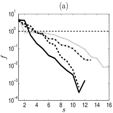
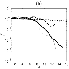
Figure 2: Ratio $f$ between the total number of avalanches in the controlled and uncontrolled situations, for several control schemes. Both in panel (a) as in (b), the following notation is used to identify parameter values and adopted control scheme: $(p_{I};\mathrm{cost\;scheme}/\mathrm{cost\;DP};\mathrm{scheme})$. In panel (a), $T_{I}=1$: solid (1; 1; DP), dashes (1; 1.29; max), dots (1; 1.46; min), dot-dashes (1; 1.31; ran). In panel (b), $T_{I}=8$: solid (0.11; 1; DP), dashes (0.12; 1.21; max), dots (0.12; 1.14; min), dot-dashes (0.1; 1.19; ran).

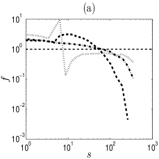
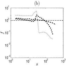
Figure 3: Ratio $f$ between the total number of avalanches in the controlled and uncontrolled situations for square lattices with size $L=32$ and for several control schemes. Both in panel (a) as in (b), the following notation is used to identify parameter values and adopted control scheme: $(p_{I};\mathrm{scheme})$. In panel (a), $T_{I}=8$: dashes (0.92; max), dots (1; min), dot-dashes (1; ran). In panel (b), $T_{I}=32$: dashes (0.33; max), dots (0.78; min), dot-dashes (0.50; ran).

4 Final remarks

We have introduced a DP approach to control SOC in the DADR model. Although this framework cannot be applied to large system, it is quite useful to characterize the optimal solution and evaluate optimality of other heuristics. The reduction in the number of large avalanches shown in Fig. 2 is similar to those obtained in [cajand10], where a fixed heuristics was considered. In that work, no cost was associated with intervention, so that it is not possible to directly compare results predicted in Fig. 1a to larger systems. However, the sudden vanishing of $\langle s\rangle$ at $(C_{I}/C_{A})_{T}$ suggests that, for heuristic based control, a similar behavior would be observed if cost is introduced in the model. Finally, this approach can be the basis to study approximate sub-optimal approaches in the line of [bertsi96], using for instance reinforcement learning techniques.

5 Acknowledgment

The authors are grateful to the Brazilian agency CNPQ and the National Institute of Science and Technology for Complex Systems (Brazil) for financial support.

References

- [1] \harvarditemBak \harvardand Sneppen1993baksne93 Bak, P. \harvardand Sneppen, K. \harvardyearleft1993\harvardyearright. Punctuated equilibrium and criticality in a simple model of evolution, Physical Review Letters 71: 4083.
- [2] \harvarditem[Bartolozzi et al.]Bartolozzi, Leinweber \harvardand Thomas2006bar06 Bartolozzi, M., Leinweber, D. B. \harvardand Thomas, A. W. \harvardyearleft2006\harvardyearright. Scale-free avalanche dynamics in the stock market, Physica A 370: 132–139.
- [3] \harvarditemBellman1957bel57 Bellman, R. \harvardyearleft1957\harvardyearright. Dynamic programming, Princeton University Press, New Jersey.
- [4] \harvarditemBertsekas \harvardand Tsitsiklis1996bertsi96 Bertsekas, D. P. \harvardand Tsitsiklis, J. N. \harvardyearleft1996\harvardyearright. Neural dynamic programming, Athena Scientific, Belmont.
- [5] \harvarditemCajueiro2005caj05 Cajueiro, D. O. \harvardyearleft2005\harvardyearright. Agent preferences and the topology of networks, Physical Review E 72: 047104.
- [6] \harvarditemCajueiro2009caj09 Cajueiro, D. O. \harvardyearleft2009\harvardyearright. Optimal navigation in complex networks, Physical Review E 79: 046103.
- [7] \harvarditemCajueiro2010caj10 Cajueiro, D. O. \harvardyearleft2010\harvardyearright. Optimal navigation for characterizing the role of the nodes in complex networks, Physica A 389: 1945–1954.
- [8] \harvarditemCajueiro \harvardand Andrade2009cajand09 Cajueiro, D. O. \harvardand Andrade, R. F. S. \harvardyearleft2009\harvardyearright. Learning paths in complex networks, Europhysics Letters 87: 58004.
- [9] \harvarditemCajueiro \harvardand Andrade2010cajand10 Cajueiro, D. O. \harvardand Andrade, R. F. S. \harvardyearleft2010\harvardyearright. Controlling self-organized criticality in abelian sandpiles, Physical Review E 81: 015102(R).
- [10] \harvarditemCajueiro \harvardand Maldonado2008cajmal08 Cajueiro, D. O. \harvardand Maldonado, W. L. \harvardyearleft2008\harvardyearright. Role of optimization on the human dynamics of tasks execution, Physical Review E 77: 035101(R).
- [11] \harvarditemCarvalho \harvardand Iori2008carior08 Carvalho, R. \harvardand Iori, G. \harvardyearleft2008\harvardyearright. Socio-economic networks with long-range interactions, Physical Review E 78: 016110.
- [12] \harvarditem[Dall’Asta et al.]Dall’Asta, Marsili \harvardand Pin2008ast08 Dall’Asta, L., Marsili, M. \harvardand Pin, P. \harvardyearleft2008\harvardyearright. Optimization in task-completion networks, Journal of Statistical Mechanics: Theory and Experiment 2008: P02003.
- [13] \harvarditemDhar \harvardand Ramaswamy1989dha89 Dhar, D. \harvardand Ramaswamy, R. \harvardyearleft1989\harvardyearright. Exactly solved model of self organized critical phenomena, Physical Review Letters 63: 1659–1662.
- [14] \harvarditemDrossel \harvardand Schwabl1992drosch92 Drossel, B. \harvardand Schwabl, F. \harvardyearleft1992\harvardyearright. Self-organized critical forest-fire model, Physical Review Letters 69: 1629.
- [15] \harvarditem[Frette et al.]Frette, Christensen, Malthe-Sorenssen, Feder, Jossang \harvardand Meakin1996fre96 Frette, V., Christensen, K., Malthe-Sorenssen, A., Feder, J., Jossang, T. \harvardand Meakin, P. \harvardyearleft1996\harvardyearright. Avalanche dynamics in a pile of rice, Nature 379: 49.
- [16] \harvarditemGreenspan2008greenspan08 Greenspan, A. \harvardyearleft2008\harvardyearright. The Age of Turbulence: Adventures in a New World, Penguin.
- [17] \harvarditemJackson \harvardand Rogers2005jacrog05 Jackson, M. O. \harvardand Rogers, B. W. \harvardyearleft2005\harvardyearright. The economics of small worlds, Journal of the European Economic Association 3: 617–627.
- [18] \harvarditemMcClung \harvardand Schaerer1993mccsch93 McClung, D. \harvardand Schaerer, P. \harvardyearleft1993\harvardyearright. The avalanche handbook, The Mountaineers, Seattle.
- [19] \harvarditemMotter \harvardand Toroczkai2007mottor07 Motter, A. E. \harvardand Toroczkai, Z. \harvardyearleft2007\harvardyearright. Introduction: Optimization in networks, Chaos 17: 026101.
- [20] \harvarditemPuterman2005put05 Puterman, M. L. \harvardyearleft2005\harvardyearright. Markov Decision Processes: Discrete Stochastic Dynamic Programming, Wiley-Interscience.
- [21] \harvarditem[Rodriguez-Iturbe et al.]Rodriguez-Iturbe, Rinaldo, Rigon, Bras, Ijjaszvasquez \harvardand Marani1992rodrin92 Rodriguez-Iturbe, I., Rinaldo, A., Rigon, R., Bras, R. L., Ijjaszvasquez, E. \harvardand Marani, A. \harvardyearleft1992\harvardyearright. Fractal structures as least energy patterns - the case of river networks, Geophysical Research Letters 19: 889–892.
- [22] \harvarditemScholz1991sch91 Scholz, C. H. \harvardyearleft1991\harvardyearright. The mechanics of earthquakes and faulting, Cambridge University Press, Cambridge.
- [23]