Stochastic gene expression with delay

Abstract

The expression of genes usually follows a two-step procedure. First, a gene (encoded in the genome) is transcribed resulting in a strand of (messenger) RNA. Afterwards, the RNA is translated into protein. We extend the classical stochastic jump model by adding delays (with arbitrary distributions) to transcription and translation.

Already in the classical model, production of RNA and protein come in bursts by activation and deactivation of the gene, resulting in a large variance of the number of RNA and proteins in equilibrium. We derive precise formulas for this second-order structure with the model including delay in equilibrium.

1 Introduction

The central dogma of molecular biology is that a gene (encoded within the genome) is transcribed into (messenger) RNA (also abbreviated mRNA), which in turn is translated into protein, the whole process also being called gene expression. Mathematical models for this process have by now been studied for a long time; see e.g. Rigney and Schieve (1977), Berg (1978), McAdams and Arkin (1997), Swain et al. (2002), Paulsson (2005), Cottrell et al. (2012), Bokes et al. (2012), Pendar et al. (2013), Fromion et al. (2013).

Within a single cell, gene expression often comes with stochastic fluctuations; see e.g. Raser and O’Shea (2005); A and van Oudenaarden (2008); Balazsi et al. (2011). There are either one or two copies of the genome, and only a few genes code for the same protein. As reviewed by Jackson et al. (2000) the majority of expressed RNA species in mammalian cells have less than 10 copies, though there are also RNA species present at an order of 10000 copies. Guptasarma (1995) observed that for 80% of genes in E. Coli genome the copy number of many proteins is less than 100. Hence in many cases there are only a small copy numbers of RNA and protein molecules, making them a noisy (i.e. stochastic) quantity. While this stochasticity has been assumed to be detrimental to the cellular function, it can also help a cell to adapt to fluctuating environments, or help to explain genetically homogeneous but phenotypically heterogeneous cellular populations (Kaern et al., 2005).

In order to consider stochasticity in gene expression, Swain et al. (2002) distinguish between intrinsic and extrinsic noise. The latter accounts for changing environments of the cell, while the former accounts for the stochastic process of transcription and translation. Let us look at the possible sources of intrinsic noise in more detail; see e.g. Zhu et al. (2007), Roussel and Zhu (2006a).
(i) Various mechanisms for gene expression require random events to occur. In order to understand this let us have a closer look at the mechanisms of gene expression. Transcription starts when RNA polymerase (which are enzymes helping in the synthetisis of RNA) binds to the promoter region of the gene, forming an elongation complex. This elongation complex is then ready to start walking along the DNA, reading off DNA and making RNA. Before the transcript is released, a ribosome binding site (which is needed for translation) is being produced on the transcript. Then follows translation which starts when a free ribosome binds to the ribosome binding site of the transcript and again is a complex process involving many chemical reactions, which lead to fluctuations.
(ii) Another source of noise comes from turning genes on and off. This means that transcription factors can bind to promoter regions of the gene and only bound (or unbound) promoters can initiate transcription. This process has been found to be the most important source of randomness for gene expression (see e.g. Swain et al., 2002; Kærn et al., 2005; Zhu and Salahub, 2008; Raj and ”van Oudenaarden”, 2008; Iyer-Biswas et al., 2009). The effect of this activation and inactivation of genes is a burst-like behavior of protein production, already apparent in McAdams and Arkin (1997). When considering the amount of RNA within the cell during the production of a specific protein, it is hence not surprising that production of RNA comes in bursts, which are related to times when the gene is turned on. This burst-like behavior is inherited to protein formation, which also comes in bursts during translation.

The classical model of stochasticity in gene expression uses exponential waiting times between transcription and translation events, and once produced, RNA and protein molecules are immediately available to the system. The latter contradicts several biological facts, valid in prokaryotes as well as in eukaryotes, e.g.: Production of RNA consists of many enzymatic reactions (Roussel and Zhu, 2006a). In the translation process another set of reactions unbinds RNA from the ribosome. For eukaryotes, post-transcriptional modification of RNA and the transport of RNA out of the nucleus to the ribosomes, as well as folding of proteins, requires time. Taking such issues into account, it makes sense to model a (random) time delay before an RNA or protein molecule can be used by the system. In our paper, we are studying the effect of (random) delay on the noise in gene expression. In real-life applications, models for such gene expression delays have been considered e.g. by Lewis (2003), Monk (2003), Barrio et al. (2006), Bratsun et al. (2005).

While our modeling approach only takes a single gene/RNA/protein triple into account, the field of systems biology aims at unraveling interactions between genes in so-called pathways. It seems clear that randomness as well as delays can accumulate in such networks of interacting genes and proteins. As a simple example, the transcription factor regulating the expression of gene $A$ is coded by a gene $B$ which in turn may be regulated by gene $A$ (or by itself), which can lead to a bi-modal distribution of the number of proteins encoded by gene $A$ or $B$; see e.g. Kaern et al. (2005). Although such feedback systems are highly interesting, we are not touching on this level of complexity.

Today, delays in biochemical reaction networks also serve as a tool for model reduction. Barrio et al. (2013) and Leier et al. (2014) argue that lumping together certain reactions effectively leads to a delay for other reactions. At least for first order reactions, they compute the resulting delay times which serve for a precise model reduction.

Simulation of chemical systems, or in silico modeling, today paves the way to understanding complex cellular processes. While the Gillespie algorithm is a classical approach for stochastic simulations (Gillespie, 1977) – see also the review Gillespie et al. (2013) – chemical delay models have as well been algorithmically studied. Various explicit simulation schemes for delay models – in particular in the field of stochasticity in gene expression – have been given; see Bratsun et al. (2005), Roussel and Zhu (2006b), Barrio et al. (2006), Cai (2007), Tian et al. (2007), Anderson (2007), Ribeiro (2010), Tian (2013), Zavala and Marquez-Lago (2014).

The goal of this paper is to give a quantitative evaluation of delay in the standard model of stochastic gene expression. We do this in a general way in which the delay – both for transcription and translation – can have an arbitrary distribution. Although we give a full description of the stochastic processes of the total number of RNA and protein molecules, our quantitative results are restricted since we only address the calculation of the first two moments (expectation, variance and autocovariances) of the number of RNA and protein molecules.

Outline: In Section 2, we introduce our delay model using a classical approach of stochastic time-change equations as well as a description of the system in equilibrium. Then, we present our main results in Section 3. Basically, Theorems 3.2 and 3.4 give the second-order structure of the number of RNA and protein in equilibrium under the delay model, respectively. In Section 4, we give several examples (uniformly and exponentially distributed delay, and delay with small variance). We end our paper with a discussion and connections to previous work in Section 5.

2 The model

In order to be able to model gene expression in a sophisticated way, we now give our delay model. Using the terminology from Roussel (1996), we may write

$$\operatorname{inactive\;gene} \autorightleftharpoons{$\lambda_1^+$}{$\lambda_1^-$}\operatorname{active\;gene}$$ (1)

$$\operatorname{active\;gene}(t) \autorightarrow{$\lambda_2$}{}\operatorname{active\;gene}(t)+\operatorname{RNA\;transcript}(t+G_{2})$$

$$\operatorname{RNA\;transcript}(t) \autorightarrow{$\lambda_3$}{}\operatorname{RNA\;transcript}(t)+\operatorname{protein}(t+G_{3})$$

$$\operatorname{RNA\;transcript} \autorightarrow{$1/\tau_2$}{}\emptyset$$

$$\operatorname{protein} \autorightarrow{$1/\tau_3$}{}\emptyset.$$

Essentially, (1) is an extension of the well-studied model of gene expression, as e.g. given in Paulsson (2005). Gene expression of $n_{\text{max}}$ similar genes is studied. Each gene is activated and deactivated at rates $\lambda_{1}^{+}$ and $\lambda_{1}^{-}$, respectively. (Additionally, we will set $\tau_{1}=1/(\lambda_{1}^{+}+\lambda_{1}^{-})$). Every active gene creates the RNA transcript at rate $\lambda_{2}$, which is degraded at rate $1/\tau_{2}$. However, a RNA molecule is available for the system (i.e. can be translated) only some random delay time $G_{2}$ after its creation, where $G_{2}$ is an independent random variable with distribution $\mu$. Then, each RNA transcript available for the system initiates translation of protein at rate $\lambda_{3}$ which in turn degrades at rate $1/\tau_{3}$. Again, it takes a delay of a random time $G_{3}$, distributed according to $\nu$ and independent of everything else, that the protein molecule is available for the system (i.e. for other downstream processes).

We note that (1) is a special case of a model studied in Zhu et al. (2007). Since they consider the ribosome binding site as an own chemical species, their model requires more delay random variables. Moreover, they distinguish gene expression in prokaryotes (bacteria) and eukaryotes (higher organisms), the main difference being that only eukaryotes have a cellular core. As a consequence, in prokaryotes translation can already be initiated when transcription is not complete yet. (The ribosome can bind to the ribosome binding site while the RNA transcript is still being produced.) The simplification (6) and (7) in Zhu et al. (2007) for gene expression in prokaryotes (both, the time the promoter region of the gene is occupied and the time the ribosome binds to the ribosome binding site are negligible), are in line with (1) for $G_{2}=0$. In addition, for the same simplification in eukaryotes (see their equation (5), where the ribosome binding site is available for binding to the ribosome only some time after the promoter was released), we exactly recover (1) for general $G_{2}$.

The question we ask is about the equilibrium behavior of the number of available RNA molecules and proteins. We restrict our study to $n_{\text{max}}=1$, because all genes are independent. We define, with $t\in\mathbb{R}$,

$$\mathcal{N}_{1}(t) =\text{number of active genes (either 0 or 1) at time $t$},$$

$$\mathcal{N}_{2}(t) =\text{number of available RNA at time $t$},$$

$$\mathcal{N}_{3}(t) =\text{number of available proteins at time $t$}.$$

Putting (1) into well-established time-change equations (Anderson and Kurtz, 2011), in equilibrium we get

$$\mathcal{N}_{1}(t) =\mathcal{P}_{1}\Big{(}\int_{-\infty}^{t}\lambda_{1}^{+}1_{\mathcal{N}_{1}(s)=0}ds\Big{)}-\mathcal{P}_{2}\Big{(}\int_{-\infty}^{t}\lambda_{1}^{-}1_{\mathcal{N}_{1}(s)=1}ds\Big{)},$$ (2)

$$\mathcal{N}_{2}(t) =\mathcal{P}_{3}\Big{(}\int_{-\infty}^{t}\int_{0}^{\infty}\lambda_{2}\mathcal{N}_{1}(s-\delta)\mu(d\delta)ds\Big{)}-\mathcal{P}_{4}\Big{(}\int_{-\infty}^{t}\frac{1}{\tau_{2}}\mathcal{N}_{2}(s)ds\Big{)},$$

$$\mathcal{N}_{3}(t) =\mathcal{P}_{5}\Big{(}\int_{-\infty}^{t}\int_{0}^{\infty}\lambda_{3}\mathcal{N}_{2}(s-\delta^{\prime})\nu(d\delta^{\prime})ds\Big{)}-\mathcal{P}_{6}\Big{(}\int_{-\infty}^{t}\frac{1}{\tau_{3}}\mathcal{N}_{3}(s)ds\Big{)}$$

for independent, unit rate Poisson processes $\mathcal{P}_{1},...,\mathcal{P}_{6}$. (Here, for the measure $\mu$, we use the standard notation $\mu(d\delta)$ for the mass the measure $\mu$ puts on the small interval $d\delta$.) Formally, we need to write integrals $\int_{-T}^{t}ds$ and then obtain the equilibrium by letting $T\to\infty$. Since we start the process at time $-\infty$, the initial state is of no relevance due to recurrence of the process. Also note that Anderson and Kurtz (2011) indicate that such delay time-change equations do have a unique solution which is shown by the same jump by jump argument as for models without delay. Another description gives the distribution of RNA and protein in equilibrium. If the gene is active, only some random delay time $G_{2}\geq 0$ with distribution $\mu$ later, the RNA is available. Therefore,

$$\mathcal{N}_{2}(t) \sim Poi\left\{\lambda_{2}\int_{0}^{\infty}e^{-\frac{r}{\tau_{2}}}\int_{0}^{\infty}\mathcal{N}_{1}(t-r-\delta)\mu(d\delta)dr\right\}$$ (3)

$$=Poi\left\{\lambda_{2}\tau_{2}\int_{0}^{\infty}\mathcal{N}_{1}(t-s)\Big{(}\exp\Big{(}\frac{1}{\tau_{2}}\Big{)}\ast\mu\Big{)}(ds)\right\},$$

where $\exp(1/\tau)$ is the exponential distribution with expectation $\tau$ and $\ast$ denotes the convolution of measures. Indeed, every RNA available at time $t$ was produced at some time $t-r$, which only works if at time $t-r-G_{2}$ (where $G_{2}\sim\mu$), the gene was active. In addition, the RNA must not be degraded during time $r$, which happens with probability $e^{-r/\tau_{2}}$. Using the same kind of arguments, we set for another delay $G_{3}\geq 0$ with distribution $\nu$

$$\mathcal{N}_{3}(t)\sim Poi\left\{\lambda_{3}\int_{0}^{\infty}e^{-\frac{r}{\tau_{3}}}\int_{0}^{\infty}\mathcal{N}_{2}(t-r-\delta)\nu(d\delta)dr\right\}$$ (4)

$$=Poi\left\{\lambda_{3}\tau_{3}\int_{0}^{\infty}\mathcal{N}_{2}(t-s)\Big{(}\exp\Big{(}\frac{1}{\tau_{3}}\Big{)}\ast\nu\Big{)}(ds)\right\}.$$

Frequently (see e.g. Paulsson, 2005; Bokes et al., 2012,) stochasticity in gene expression is studied through the Master equation. We stress that the usual Master equation is unsuitable to be used for an arbitrary delay of RNA and protein production. The reason is simply that by a non-exponentially distributed delay, the process $(\mathcal{N}_{1},\mathcal{N}_{2},\mathcal{N}_{3})$ is not a Markov process; however, compare with Tian et al. (2007) where an extension of the Master equation for deterministic delay models is given. Note that our Poisson point process approach is similar in spirit to Fromion et al. (2013), who model an arbitrary (non-exponential) life-time distribution of RNA and protein using point processes but without delay.

We remark that our modeling is unrealistic at least in one respect: considering two RNA molecules, created at times $s$ and $s^{\prime}$ with $s<s^{\prime}$, both will be available for translation by times $t=s+G_{2}$ and $t^{\prime}=s^{\prime}+G_{2}^{\prime}$. However, since the delay for both RNA molecules is given through independent $G_{2}$ and $G_{2}^{\prime}$, both having distribution $\mu$, it might be that $t>t^{\prime}$.

From (2), (3) and (4), we already obtain the equilibrium expectations and second moments in Proposition 3.1, Theorem 3.2 and 3.4. We will see that expectations are independent of the delay distributions, $\mu$ and $\nu$. This situation will change for the second-order structure.

3 Results

We are now ready to formulate and prove our results on the number of active genes (Proposition 3.1), the amount of RNA molecules (Theorem 3.2) and the number of available protein (Theorem 3.4). We start with first and second moments of the active genes.

Proposition 3.1 (First and second order structure of $\mathcal{N}_{1}$).

The expectation, variance and covariance of $\mathcal{N}_{1}$ in equilibrium are given by

$$\mathbf{E}[\mathcal{N}_{1}(t)] =\lambda_{1}^{+}\tau_{1},$$ (5)

$$\mathbf{Cov}[\mathcal{N}_{1}(0),\mathcal{N}_{1}(t)] =e^{-\frac{|t|}{\tau_{1}}}\lambda_{1}^{+}\lambda_{1}^{-}\tau_{1}^{2},$$ (6)

$$\mathbf{Var}[\mathcal{N}_{1}(t)] =\lambda_{1}^{+}\lambda_{1}^{-}\tau_{1}^{2}.$$ (7)

Proof.

Since activation and de-actication of the gene is independent of downstream processes, the assertion follows by a simple calculation using Poisson processes. We omit the details. ∎

Next, we derive our results for the amount of RNA.

Theorem 3.2 (Expectation, variance and covariance of RNA in equilibrium).

The expectation, variance and covariance of $\mathcal{N}_{2}$ in equilibrium are given by

$$\mathbf{E}[\mathcal{N}_{2}(t)] =\lambda_{1}^{+}\lambda_{2}\tau_{1}\tau_{2},$$ (8)

$$\mathbf{Cov}[\mathcal{N}_{2}(0),\mathcal{N}_{2}(t)] =\lambda_{1}^{+}\lambda_{2}\tau_{1}\tau_{2}e^{-\frac{|t|}{\tau_{2}}}$$ (9)

$$+\lambda_{1}^{+}\lambda_{1}^{-}\lambda_{2}^{2}\tau_{1}^{2}\tau_{2}^{2}\frac{\tau_{1}}{\tau_{1}+\tau_{2}}\frac{\tau_{1}\mathbf{E}\Big{[}e^{-\frac{|G_{2}^{\prime}-G_{2}-|t||}{\tau_{1}}}\Big{]}-\tau_{2}\mathbf{E}\Big{[}e^{-\frac{|G_{2}^{\prime}-G_{2}-|t||}{\tau_{2}}}\Big{]}}{\tau_{1}-\tau_{2}},$$

$$\mathbf{Var}[\mathcal{N}_{2}(t)] =\lambda_{1}^{+}\lambda_{2}\tau_{1}\tau_{2}$$ (10)

$$\qquad+\lambda_{1}^{+}\lambda_{1}^{-}\lambda_{2}^{2}\tau_{1}^{2}\tau_{2}^{2}\frac{\tau_{1}}{\tau_{1}+\tau_{2}}\cdot\frac{\tau_{1}\mathbf{E}\Big{[}e^{-\frac{|G_{2}^{\prime}-G_{2}|}{\tau_{1}}}\Big{]}-\tau_{2}\mathbf{E}\Big{[}e^{-\frac{|G_{2}^{\prime}-G_{2}|}{\tau_{2}}}\Big{]}}{\tau_{1}-\tau_{2}},$$

where $G_{2},G^{\prime}_{2}$ are independent and $G_{2},G^{\prime}_{2}\sim\mu$.

Remark 3.3 (Convexity and deterministic delay).

We note that the last terms in (9) and (10) stay bounded, even for $\tau_{1}\to\tau_{2}$. Moreover, for $X\geq 0$ the map $t\mapsto\mathbf{E}[e^{-Xt}]$ is convex. Hence, assuming $\tau_{1}>\tau_{2}$ without loss of generality, we obtain, using the convex combination $1=\frac{\tau_{1}}{\tau_{1}-\tau_{2}}-\frac{\tau_{2}}{\tau_{1}-\tau_{2}}$ (and noting that $\frac{\tau_{1}}{\tau_{1}-\tau_{2}}>1$) that for a random variable $S$

$$f_{S}(\tau_{1},\tau_{2}) :=\frac{\tau_{1}\mathbf{E}\Big{[}e^{-\frac{S}{\tau_{1}}}\Big{]}-\tau_{2}\mathbf{E}\Big{[}e^{-\frac{S}{\tau_{2}}}\Big{]}}{\tau_{1}-\tau_{2}}$$ (11)

$$\qquad\leq\mathbf{E}\Big{[}\exp\Big{(}-\Big{(}\frac{1}{\tau_{1}}\frac{\tau_{1}}{\tau_{1}-\tau_{2}}-\frac{1}{\tau_{2}}\frac{\tau_{2}}{\tau_{1}-\tau_{2}}\Big{)}S\Big{)}\Big{]}=1$$

with equality if and only if $\mathbf{V}[S]=0$. In particular we see that

$$\mathbf{Var}[\mathcal{N}_{2}(t)]\leq\lambda_{1}^{+}\lambda_{2}\tau_{1}\tau_{2}+\lambda_{1}^{+}\lambda_{1}^{-}\lambda_{2}^{2}\tau_{1}^{2}\tau_{2}^{2}\frac{\tau_{1}}{\tau_{1}+\tau_{2}}$$

with equality if and only if $\mu$ is a delta-measure. In particular, we see that stochastic delay leads to a decrease in the variance for $\mathcal{N}_{2}$ in equilibrium. For a deterministic delay, we obtain

$$\frac{\mathbf{Var}[\mathcal{N}_{2}(t)]}{\mathbf{E}[\mathcal{N}_{2}(t)]^{2}} =\frac{1}{\mathbf{E}[\mathcal{N}_{2}(t)]}+\frac{\lambda_{1}^{+}\lambda_{1}^{-}\lambda_{2}^{2}\tau_{1}^{3}\tau_{2}^{2}}{(\tau_{1}+\tau_{2})\lambda_{2}^{2}(\lambda_{1}^{+})^{2}\tau_{1}^{2}\tau_{2}^{2}}=\frac{1}{\mathbf{E}[N_{2}]}+\frac{\lambda_{1}^{-}}{\lambda_{1}^{+}}\frac{\tau_{1}}{\tau_{1}+\tau_{2}},$$

which equals the numerical value in the absence of delay, $\mu=\delta_{0}$; see equation (5) in Paulsson (2005).

Proof of Theorem 3.2.

Using (3) and Proposition 3.1, we write

$$\mathbf{E}[\mathcal{N}_{2}(t)] =\mathbf{E}\left[\lambda_{2}\tau_{2}\int_{0}^{\infty}\mathcal{N}_{1}(t-s)\Big{(}\exp\Big{(}\frac{1}{\tau_{2}}\Big{)}\ast\mu\Big{)}(ds)\right]$$

$$=\lambda_{2}\tau_{2}\int_{0}^{\infty}\mathbf{E}[\mathcal{N}_{1}(t-s)]\Big{(}\exp\Big{(}\frac{1}{\tau_{2}}\Big{)}\ast\mu\Big{)}(ds)$$

$$=\lambda_{2}\tau_{2}\lambda_{1}^{+}\tau_{1}.$$

For (9) and (10), it clearly suffices to prove (9), since the variance formula just requires to take $t=0$. From our model, we can write in the case $t\geq 0$ (compare with the explanation given below (3))

$$\mathcal{N}_{2}(0) =X+Y,$$

$$\mathcal{N}_{2}(t) =X+Z,$$

where $X,Y$ and $Z$ are conditionally independent given $\mathcal{N}_{1}$ such that

$$X \sim Poi\left\{\lambda_{2}\int_{0}^{\infty}e^{-\frac{r+t}{\tau_{2}}}\int_{0}^{\infty}\mathcal{N}_{1}(-r-\delta)\mu(d\delta)dr\right\}$$

$$=Poi\left\{\lambda_{2}\tau_{2}e^{-\frac{t}{\tau_{2}}}\int_{0}^{\infty}\mathcal{N}_{1}(-s)\Big{(}\exp\Big{(}\frac{1}{\tau_{2}}\Big{)}\ast\mu\Big{)}(ds)\right\}$$

is the number of RNAs available by time $0$ which will not be degraded by time $t$,

$$Y \sim Poi\left\{\lambda_{2}\int_{0}^{\infty}e^{-\frac{r}{\tau_{2}}}(1-e^{-\frac{t}{\tau_{2}}})\int_{0}^{\infty}\mathcal{N}_{1}(-r-\delta)\mu(d\delta)dr\right\}$$

$$=Poi\left\{\lambda_{2}\tau_{2}\big{(}1-e^{-\frac{t}{\tau_{2}}}\big{)}\int_{0}^{\infty}\mathcal{N}_{1}(-s)\Big{(}\exp\Big{(}\frac{1}{\tau_{2}}\Big{)}\ast\mu\Big{)}(ds)\right\}$$

is the number of RNAs available by time $0$ which will be degraded by time $t$,

$$Z \sim Poi\left\{\lambda_{2}\int_{0}^{t}e^{-\frac{r}{\tau_{2}}}\int_{0}^{\infty}\mathcal{N}_{1}(t-r-\delta)\mu(d\delta)dr\right\}$$

$$=Poi\left\{\lambda_{2}\int_{0}^{\infty}e^{-\frac{r}{\tau_{2}}}1_{r\leq t}\int_{0}^{\infty}\mathcal{N}_{1}(t-r-\delta)\mu(d\delta)dr\right\}$$

is the number of RNAs available only after time $0$ and present by time $t$.

Hence, we get

$$\mathbf{Cov}[ \mathcal{N}_{2}(0),\mathcal{N}_{2}(t)]=\mathbf{Cov}[X+Y,X+Z]$$

$$=\mathbf{E}\big{[}\mathbf{Var}[X|\mathcal{N}_{1}]\big{]}+\mathbf{Var}\big{[}\mathbf{E}[X|\mathcal{N}_{1}]\big{]}+\mathbf{Cov}\big{[}\mathbf{E}[X|\mathcal{N}_{1}],\mathbf{E}[Z|\mathcal{N}_{1}]\big{]}$$

$$\qquad\qquad\qquad\qquad+\mathbf{Cov}\big{[}\mathbf{E}[X|\mathcal{N}_{1}],\mathbf{E}[Y|\mathcal{N}_{1}]\big{]}+\mathbf{Cov}\big{[}\mathbf{E}[Y|\mathcal{N}_{1}],\mathbf{E}[Z|\mathcal{N}_{1}]\big{]}$$

$$=\mathbf{E}\Big{[}\lambda_{2}\tau_{2}e^{-\frac{t}{\tau_{2}}}\int_{0}^{\infty}\mathcal{N}_{1}(-s)\Big{(}\exp\Big{(}\frac{1}{\tau_{2}}\Big{)}\ast\mu\Big{)}(ds)\Big{]}$$

$$\qquad+\mathbf{Var}\Big{[}\lambda_{2}\tau_{2}e^{-\frac{t}{\tau_{2}}}\int_{0}^{\infty}\mathcal{N}_{1}(-s)\Big{(}\exp\Big{(}\frac{1}{\tau_{2}}\Big{)}\ast\mu\Big{)}(ds)\Big{]}$$

$$\qquad+\mathbf{Cov}\Big{[}\lambda_{2}\tau_{2}e^{-\frac{t}{\tau_{2}}}\int_{0}^{\infty}\mathcal{N}_{1}(-s)\Big{(}\exp\Big{(}\frac{1}{\tau_{2}}\Big{)}\ast\mu\Big{)}(ds),$$

$$\qquad\qquad\qquad\qquad\qquad\qquad\qquad\qquad\lambda_{2}\int_{0}^{\infty}e^{-\frac{r}{\tau_{2}}}1_{r\leq t}\int_{0}^{\infty}\mathcal{N}_{1}(t-r-\delta)\mu(d\delta)dr\Big{]}$$

$$\qquad+\mathbf{Cov}\Big{[}\lambda_{2}\tau_{2}e^{-\frac{t}{\tau_{2}}}\int_{0}^{\infty}\mathcal{N}_{1}(-s)\Big{(}\exp\Big{(}\frac{1}{\tau_{2}}\Big{)}\ast\mu\Big{)}(ds),$$

$$\qquad\qquad\qquad\qquad\qquad\qquad\lambda_{2}\tau_{2}\big{(}1-e^{-\frac{t}{\tau_{2}}}\big{)}\int_{0}^{\infty}\mathcal{N}_{1}(-s)\Big{(}\exp\Big{(}\frac{1}{\tau_{2}}\Big{)}\ast\mu\Big{)}(ds)\Big{]}$$

$$\qquad+\mathbf{Cov}\Big{[}\lambda_{2}\tau_{2}\big{(}1-e^{-\frac{t}{\tau_{2}}}\big{)}\int_{0}^{\infty}\mathcal{N}_{1}(-s)\Big{(}\exp\Big{(}\frac{1}{\tau_{2}}\Big{)}\ast\mu\Big{)}(ds),$$

$$\qquad\qquad\qquad\qquad\qquad\qquad\qquad\lambda_{2}\int_{0}^{\infty}e^{-\frac{r}{\tau_{2}}}1_{r\leq t}\int_{0}^{\infty}\mathcal{N}_{1}(t-r-\delta)\mu(d\delta)dr\Big{]}$$

$$=:A_{1}+A_{2}+A_{3}+A_{4}+A_{5}.$$

We treat the terms separately and write, using Proposition 3.1, for independent, $\exp(1/\tau_{2})$-distributed random variables $T_{2},T_{2}^{\prime}$,

$$A_{1} =\lambda_{1}^{+}\lambda_{2}\tau_{1}\tau_{2}e^{-\frac{t}{\tau_{2}}},$$

$$A_{2}+A_{4} =\lambda_{2}^{2}\tau_{2}^{2}\big{(}e^{-\frac{2t}{\tau_{2}}}+e^{-\frac{t}{\tau_{2}}}\big{(}1-e^{-\frac{t}{\tau_{2}}}\big{)}\int_{0}^{\infty}\int_{0}^{\infty}\mathbf{Cov}[\mathcal{N}_{1}(-s),\mathcal{N}_{1}(-r)]$$

$$\qquad\qquad\qquad\qquad\qquad\qquad\qquad\Big{(}\exp\Big{(}\frac{1}{\tau_{2}}\Big{)}\ast\mu\Big{)}(ds)\Big{(}\exp\Big{(}\frac{1}{\tau_{2}}\Big{)}\ast\mu\Big{)}(dr)$$

$$=\lambda_{1}^{+}\lambda_{1}^{-}\lambda_{2}^{2}\tau_{1}^{2}\tau_{2}^{2}e^{-\frac{t}{\tau_{2}}}\iint e^{-\frac{|s-r|}{\tau_{1}}}\Big{(}\exp\Big{(}\frac{1}{\tau_{2}}\Big{)}\ast\mu\Big{)}(ds)\Big{(}\exp\Big{(}\frac{1}{\tau_{2}}\Big{)}\ast\mu\Big{)}(dr)$$

$$=\lambda_{1}^{+}\lambda_{1}^{-}\lambda_{2}^{2}\tau_{1}^{2}\tau_{2}^{2}e^{-\frac{t}{\tau_{2}}}\mathbf{E}\Big{[}e^{-\frac{|T_{2}+G-T_{2}^{\prime}-G^{\prime}|}{\tau_{1}}}\Big{]},$$

$$A_{3}+A_{5} =\lambda_{2}^{2}\tau_{2}^{2}\iiint 1_{r\leq t}\mathbf{Cov}[\mathcal{N}_{1}(-s),\mathcal{N}_{1}(t-r-\delta)]\mu(d\delta)\exp\Big{(}\frac{1}{\tau_{2}}\Big{)}(dr)$$

$$\qquad\qquad\qquad\qquad\qquad\qquad\qquad\qquad\qquad\qquad\qquad\Big{(}\exp\Big{(}\frac{1}{\tau_{2}}\Big{)}\ast\mu\Big{)}(ds)$$

$$=\lambda_{1}^{+}\lambda_{1}^{-}\lambda_{2}^{2}\tau_{1}^{2}\tau_{2}^{2}\iiint 1_{r\leq t}e^{-\frac{|t+s-r-\delta|}{\tau_{1}}}\mu(d\delta)\exp\Big{(}\frac{1}{\tau_{2}}\Big{)}(dr)$$

$$\qquad\qquad\qquad\qquad\qquad\qquad\qquad\qquad\qquad\qquad\qquad\Big{(}\exp\Big{(}\frac{1}{\tau_{2}}\Big{)}\ast\mu\Big{)}(ds)$$

$$=\lambda_{1}^{+}\lambda_{1}^{-}\lambda_{2}^{2}\tau_{1}^{2}\tau_{2}^{2}\mathbf{E}\Big{[}e^{-\frac{|t+T_{2}+G-T_{2}^{\prime}-G^{\prime}|}{\tau_{1}}},T_{2}^{\prime}\leq t\Big{]}$$

$$=\lambda_{1}^{+}\lambda_{1}^{-}\lambda_{2}^{2}\tau_{1}^{2}\tau_{2}^{2}\Big{(}\mathbf{E}\Big{[}e^{-\frac{|t+T_{2}+G-T_{2}^{\prime}-G^{\prime}|}{\tau_{1}}}\Big{]}-\mathbf{E}\Big{[}e^{-\frac{|t+T_{2}+G-T_{2}^{\prime}-G^{\prime}|}{\tau_{1}}}\Big{|}T_{2}^{\prime}>t\Big{]}e^{-\frac{t}{\tau_{2}}}\Big{)}$$

$$=\lambda_{1}^{+}\lambda_{1}^{-}\lambda_{2}^{2}\tau_{1}^{2}\tau_{2}^{2}\Big{(}\mathbf{E}\Big{[}e^{-\frac{|t+T_{2}+G-T_{2}^{\prime}-G^{\prime}|}{\tau_{1}}}\Big{]}-\mathbf{E}\Big{[}e^{-\frac{|T_{2}+G-T_{2}^{\prime}-G^{\prime}|}{\tau_{1}}}\Big{]}e^{-\frac{t}{\tau_{2}}}\Big{)}$$

because, given $T_{2}^{\prime}>t$, the random variable $T_{2}^{\prime}-t$ is exp$\Big{(}\frac{1}{\tau_{2}}\Big{)}$-distributed. Altogether,

$$\mathbf{Cov}[\mathcal{N}_{2}(0),\mathcal{N}_{2}(t)]=\lambda_{1}^{+}\lambda_{2}\tau_{1}\tau_{2}e^{-\frac{|t|}{\tau_{2}}}+\lambda_{1}^{+}\lambda_{1}^{-}\lambda_{2}^{2}\tau_{1}^{2}\tau_{2}^{2}\mathbf{E}\Big{[}e^{-\frac{||t|+T_{2}+G-T_{2}^{\prime}-G^{\prime}|}{\tau_{1}}}\Big{]}.$$ (12)

Now, (9) follows since by Lemma A.1,

$$\mathbf{E}\Big{[} e^{-\frac{||t|+T_{2}+G-T_{2}^{\prime}-G^{\prime}|}{\tau_{1}}}\Big{]}$$

$$=\frac{\tau_{1}}{(\tau_{1}+\tau_{2})(\tau_{1}-\tau_{2})}\Big{(}\tau_{1}\mathbf{E}\Big{[}e^{-\frac{|G_{2}^{\prime}-G_{2}-|t||}{\tau_{1}}}\Big{]}-\tau_{2}\mathbf{E}\Big{[}e^{-\frac{|G_{2}^{\prime}-G_{2}-|t||}{\tau_{2}}}\Big{]}\Big{)}.$$

∎

Theorem 3.4 (Expectation and variance of protein in equilibrium).

The expectation and variance of $\mathcal{N}_{3}$ in equilibrium are given by

$$\mathbf{E}[\mathcal{N}_{3}(t)]=\lambda_{1}^{+}\lambda_{2}\lambda_{3}\tau_{1}\tau_{2}\tau_{3},$$ (13)

$$\mathbf{Var}[\mathcal{N}_{3}(t)]=\lambda_{1}^{+}\lambda_{2}\lambda_{3}\tau_{1}\tau_{2}\tau_{3}+\lambda_{1}^{+}\lambda_{2}\lambda_{3}^{2}\tau_{1}\tau_{2}\tau_{3}^{2}\cdot A+\lambda_{1}^{+}\lambda_{1}^{-}\lambda_{2}^{2}\lambda_{3}^{2}\tau_{1}^{2}\tau_{2}^{2}\tau_{3}^{2}\cdot B,$$ (14)

$$A=\frac{\tau_{2}}{\tau_{2}+\tau_{3}}\frac{\tau_{2}\mathbf{E}\Big{[}e^{-\frac{|G_{3}-G_{3}^{\prime}|}{\tau_{2}}}\Big{]}-\tau_{3}\mathbf{E}\Big{[}e^{-\frac{|G_{3}-G_{3}^{\prime}|}{\tau_{3}}}\Big{]}}{\tau_{2}-\tau_{3}}$$ (15)

$$B=\frac{\tau_{1}}{\tau_{1}+\tau_{3}}\Big{(}\frac{\tau_{1}^{2}}{\tau_{1}+\tau_{2}}\frac{\tau_{1}\mathbf{E}\Big{[}e^{-\frac{|G_{3}-G_{3}^{\prime}+G_{2}-G_{2}^{\prime}|}{\tau_{1}}}\Big{]}-\tau_{2}\mathbf{E}\Big{[}e^{-\frac{|G_{3}-G_{3}^{\prime}+G_{2}-G_{2}^{\prime}|}{\tau_{2}}}\Big{]}}{(\tau_{1}-\tau_{3})(\tau_{1}-\tau_{2})}$$ (16)

$$\qquad\qquad\qquad\qquad-\frac{\tau_{3}^{2}}{\tau_{2}+\tau_{3}}\frac{\tau_{2}\mathbf{E}\Big{[}e^{-\frac{|G_{3}-G_{3}^{\prime}+G_{2}-G_{2}^{\prime}|}{\tau_{2}}}\Big{]}-\tau_{3}\mathbf{E}\Big{[}e^{-\frac{|G_{3}-G_{3}^{\prime}+G_{2}-G_{2}^{\prime}|}{\tau_{3}}}\Big{]}}{(\tau_{1}-\tau_{3})(\tau_{2}-\tau_{3})}\Big{)},$$

where $G_{2},G_{2}^{\prime},G_{3},G_{3}^{\prime}$ and independent and $G_{2},G_{2}^{\prime}\sim\mu$ and $G_{3},G_{3}^{\prime}\sim\nu$.

Remark 3.5 (Convexity and deterministic delay).

We note that the last terms in (15) and (16) stay bounded, even for $\tau_{1}\to\tau_{2}$, $\tau_{2}\to\tau_{3}$ and $\tau_{1}\to\tau_{3}$. In addition, $A,B\geq 0$ can easily be shown, which means that $\mathbf{Var}[\mathcal{N}_{3}(t)]\geq\mathbf{E}[\mathcal{N}_{3}(t)]$ in all cases. Moreover, we will – as for the second moments of the amount of RNA – argue that $\mathbf{Var}[\mathcal{N}_{3}(t)]$ is largest in the absence of delay. First, recall from (11) that $A\leq 1$ with equality if and only if $\mu$ is a delta-measure (i.e. $\mathbf{Var}[G_{2}]=0$). Moreover, for a similar bound on $B$, assume without loss of generality that $\tau_{1}>\tau_{3}$ and write, using again (11) and $S:=|G_{3}-G_{3}^{\prime}+G_{2}-G_{2}^{\prime}|$

$$\frac{\tau_{1}+\tau_{3}}{\tau_{1}}B =\frac{\tau_{1}^{2}f_{S}(\tau_{1},\tau_{2})}{(\tau_{1}+\tau_{2})(\tau_{1}-\tau_{3})}-\frac{\tau_{3}^{2}f_{S}(\tau_{2},\tau_{3})}{(\tau_{2}+\tau_{3})(\tau_{1}-\tau_{3})}$$

$$=\frac{\tau_{1}^{2}\tau_{2}f_{S}(\tau_{1},\tau_{2})+\tau_{1}^{2}\tau_{3}f_{S}(\tau_{1},\tau_{2})-\tau_{1}\tau_{3}^{2}f_{S}(\tau_{2},\tau_{3})-\tau_{2}\tau_{3}^{2}f_{S}(\tau_{2},\tau_{3})}{(\tau_{1}+\tau_{2})(\tau_{2}+\tau_{3})(\tau_{1}-\tau_{3})}$$

$$=\frac{\tau_{2}(\tau_{1}+\tau_{3})}{(\tau_{1}+\tau_{2})(\tau_{2}+\tau_{3})}\frac{\tau_{1}^{2}f_{S}(\tau_{1},\tau_{2})-\tau_{3}^{2}f_{S}(\tau_{3},\tau_{2})}{\tau_{1}^{2}-\tau_{3}^{2}}$$

$$\qquad\qquad\qquad\qquad+\frac{\tau_{1}\tau_{3}}{(\tau_{1}+\tau_{2})(\tau_{2}+\tau_{3})}\frac{\tau_{1}f_{S}(\tau_{1},\tau_{2})-\tau_{3}f_{S}(\tau_{3},\tau_{2})}{\tau_{1}-\tau_{3}}.$$

Next, it is easy to check that the function $t\mapsto f_{S}(t,\tau_{2})$ is convex. (For this, it suffices to show that $t\mapsto t\mathbf{E}[e^{-S/t}]$ is convex, which can be shown by computing two derivatives.) Therefore, using the convex combinations $1=\frac{\tau_{1}^{2}}{\tau_{1}^{2}-\tau_{3}^{2}}-\frac{\tau_{1}^{3}}{\tau_{1}^{2}-\tau_{3}^{2}}$ and $1=\frac{\tau_{1}}{\tau_{1}-\tau_{3}}-\frac{\tau_{3}}{\tau_{1}-\tau_{3}}$ (recall $\tau_{1}>\tau_{3}$), we see that

$$\frac{\tau_{1}^{2}f_{S}(\tau_{1},\tau_{2})-\tau_{3}^{2}f_{S}(\tau_{3},\tau_{2})}{\tau_{1}^{2}-\tau_{3}^{2}}$$

$$\qquad\leq f_{S}\Big{(}\frac{\tau_{3}^{2}}{\tau_{1}^{2}-\tau_{3}^{2}}-\frac{\tau_{3}^{2}}{\tau_{1}^{2}-\tau_{3}^{2}},\tau_{2}\Big{)}=f_{S}\Big{(}\frac{\tau_{1}^{2}+\tau_{1}\tau_{3}+\tau_{3}^{2}}{\tau_{1}+\tau_{3}},\tau_{2}\Big{)}\leq 1,$$

$$\frac{\tau_{1}f_{S}(\tau_{1},\tau_{2})-\tau_{3}f_{S}(\tau_{3},\tau_{2})}{\tau_{1}-\tau_{3}}$$

$$\qquad\leq f_{S}\Big{(}\frac{\tau_{1}^{2}}{\tau_{1}-\tau_{3}}-\frac{\tau_{3}^{2}}{\tau_{1}-\tau_{3}},\tau_{2}\Big{)}=f_{S}(\tau_{1}+\tau_{3},\tau_{2})\leq 1$$

with equality if and only if $\mathbf{Var}[S]=0$. In total, we see that

$$\mathbf{Var}[\mathcal{N}_{3}(t)] \leq\lambda_{1}^{+}\lambda_{2}\lambda_{3}\tau_{1}\tau_{2}\tau_{3}+\lambda_{1}^{+}\lambda_{2}\lambda_{3}^{2}\tau_{1}\tau_{2}\tau_{3}^{2}\frac{\tau_{2}}{\tau_{2}+\tau_{3}}$$

$$\qquad\qquad\qquad\qquad+\lambda_{1}^{+}\lambda_{1}^{-}\lambda_{2}^{2}\lambda_{3}^{2}\tau_{1}^{2}\tau_{2}^{2}\tau_{3}^{2}\frac{\tau_{1}}{\tau_{1}+\tau_{3}}\frac{\tau_{1}\tau_{2}+\tau_{1}\tau_{3}+\tau_{2}\tau_{3}}{(\tau_{2}+\tau_{3})(\tau_{1}+\tau_{2})}$$

with equality if $\mu$ and $\nu$ are delta-measures. In this case,

$$\frac{\mathbf{Var}[\mathcal{N}_{3}(t)]}{\mathbf{E}[\mathcal{N}_{3}(t)]^{2}} =\frac{1}{\mathbf{E}[\mathcal{N}_{3}(t)]}+\frac{1}{\lambda_{1}^{+}\lambda_{2}\tau_{1}\tau_{2}}\frac{\tau_{2}}{\tau_{2}+\tau_{3}}+\frac{\lambda_{1}^{-}}{\lambda_{1}^{+}}\frac{\tau_{1}}{\tau_{1}+\tau_{2}}\frac{\tau_{1}\tau_{2}+\tau_{1}\tau_{3}+\tau_{2}\tau_{3}}{(\tau_{2}+\tau_{3})(\tau_{1}+\tau_{3})},$$

which is a well-known result; see equation (4) in Paulsson (2005).

Proof of Theorem 3.4.

Using (4) and Theorem 3.2

$$\mathbf{E}[\mathcal{N}_{3}(t)] =\mathbf{E}\left[\lambda_{3}\tau_{3}\int_{0}^{\infty}\mathcal{N}_{2}(t-s)\Big{(}\exp\Big{(}\frac{1}{\tau_{3}}\Big{)}\ast\nu\Big{)}(ds)\right]$$

$$=\lambda_{3}\tau_{3}\lambda_{2}\lambda_{1}^{+}\tau_{1}\tau_{2}.$$

For the variance, we again use (4) and two independent $\exp(1/\tau_{3})$-distributed random variables $T_{3},T_{3}^{\prime}$ for

$$\mathbf{Var}[\mathcal{N}_{3}(t)]=\mathbf{E}\big{[}\mathbf{Var}[\mathcal{N}_{3}(t)|\mathcal{N}_{1},\mathcal{N}_{2}]\big{]}+\mathbf{Var}\big{[}\mathbf{E}[\mathcal{N}_{3}(t)|\mathcal{N}_{1},\mathcal{N}_{2}]\big{]},$$

with

$$\mathbf{E}\big{[}\mathbf{Var}[\mathcal{N}_{3}(t)|\mathcal{N}_{1},\mathcal{N}_{2}]\big{]}=\mathbf{E}\Big{[}\lambda_{3}\tau_{3}\int_{0}^{\infty}\mathcal{N}_{2}(t-r)\Big{(}\exp\Big{(}-\frac{1}{\tau_{3}}\Big{)}\ast\nu\Big{)}(dr)\Big{]}$$

$$\qquad\qquad\qquad\qquad\qquad=\lambda_{1}^{+}\lambda_{2}\lambda_{3}\tau_{1}\tau_{2}\tau_{3}$$

and with (12) in the third equality

$$\mathbf{Var}\big{[}\mathbf{E}[\mathcal{N}_{3}(t)|\mathcal{N}_{1},\mathcal{N}_{2}]\big{]}=\mathbf{Var}\Big{[}\lambda_{3}\tau_{3}\int_{0}^{\infty}\mathcal{N}_{2}(t-r)\Big{(}\exp\Big{(}\frac{1}{\tau_{3}}\Big{)}\ast\nu\Big{)}(dr)\Big{]}$$

$$=\lambda_{3}^{2}\tau_{3}^{2}\int_{0}^{\infty}\int_{0}^{\infty}\mathbf{Cov}[\mathcal{N}_{2}(t-s),\mathcal{N}_{2}(t-r)]$$

$$\qquad\qquad\qquad\qquad\qquad\Big{(}\exp\Big{(}\frac{1}{\tau_{3}}\Big{)}\ast\nu\Big{)}(dr)\Big{(}\exp\Big{(}\frac{1}{\tau_{3}}\Big{)}\ast\nu\Big{)}(ds)$$

$$=\lambda_{1}^{+}\lambda_{2}\lambda_{3}^{2}\tau_{1}\tau_{2}\tau_{3}^{2}\int_{0}^{\infty}\int_{0}^{\infty}e^{-\frac{|s-r|}{\tau_{2}}}\Big{(}\exp\Big{(}\frac{1}{\tau_{3}}\Big{)}\ast\nu\Big{)}(dr)\Big{(}\exp\Big{(}\frac{1}{\tau_{3}}\Big{)}\ast\nu\Big{)}(ds)$$

$$\qquad+\lambda_{1}^{+}\lambda_{1}^{-}\lambda_{2}^{2}\lambda_{3}^{2}\tau_{1}^{2}\tau_{2}^{2}\tau_{3}^{2}$$

$$\qquad\qquad\Big{(}\int_{0}^{\infty}\int_{0}^{\infty}\mathbf{E}\Big{[}e^{-\frac{||s-r|+T_{2}+G_{2}-T_{2}^{\prime}-G_{2}^{\prime}|}{\tau_{1}}}\Big{]}$$

$$\qquad\qquad\qquad\qquad\qquad\qquad\Big{(}\exp\Big{(}\frac{1}{\tau_{3}}\Big{)}\ast\nu\Big{)}(dr)\Big{(}\exp\Big{(}\frac{1}{\tau_{3}}\Big{)}\ast\nu\Big{)}(ds)\Big{)}$$

$$=\lambda_{1}^{+}\lambda_{2}\lambda_{3}^{2}\tau_{1}\tau_{2}\tau_{3}^{2}\mathbf{E}\Big{[}e^{-\frac{|T_{3}+G_{3}-T_{3}^{\prime}-G_{3}^{\prime}|}{\tau_{2}}}\Big{]}$$ (17)

$$\qquad+\lambda_{1}^{+}\lambda_{1}^{-}\lambda_{2}^{2}\lambda_{3}^{2}\tau_{1}^{2}\tau_{2}^{2}\tau_{3}^{2}\mathbf{E}\Big{[}e^{-\frac{||T_{3}+G_{3}-T_{3}^{\prime}-G_{3}^{\prime}|+T_{2}+G_{2}-T_{2}^{\prime}-G_{2}^{\prime}|}{\tau_{1}}}\Big{]}.$$

Now, by Lemma A.1, (20),

$$\mathbf{E}\Big{[}e^{-\frac{|T_{3}+G_{3}-T_{3}^{\prime}-G_{3}^{\prime}|}{\tau_{2}}}\Big{]} =\frac{\tau_{2}}{\tau_{2}+\tau_{3}}\frac{\tau_{2}\mathbf{E}\Big{[}e^{-\frac{|G_{3}-G_{3}^{\prime}|}{\tau_{2}}}\Big{]}-\tau_{3}\mathbf{E}\Big{[}e^{-\frac{|G_{3}-G_{3}^{\prime}|}{\tau_{3}}}\Big{]}}{\tau_{2}-\tau_{3}}$$ (18)

and by applying (21) twice (first for $S=T_{2}+G_{2}^{\prime}-T_{2}-G_{2}$ and then for $S=G_{2}-G_{2}^{\prime}+G_{3}-G_{3}^{\prime}$

$$\mathbf{E}\Big{[} e^{-\frac{||T_{3}+G_{3}-T_{3}^{\prime}-G_{3}^{\prime}|+T_{2}+G_{2}-T_{2}^{\prime}-G_{2}^{\prime}|}{\tau_{1}}}\Big{]}$$ (19)

$$=\frac{\tau_{1}}{\tau_{1}+\tau_{3}}\frac{\tau_{1}\mathbf{E}\Big{[}e^{-\frac{|T_{2}+G_{2}-T_{2}^{\prime}-G_{2}^{\prime}+G_{3}-G_{3}^{\prime}|}{\tau_{1}}}\Big{]}-\tau_{3}\mathbf{E}\Big{[}e^{-\frac{|T_{2}+G_{2}-T_{2}^{\prime}-G_{2}^{\prime}+G_{3}-G_{3}^{\prime}|}{\tau_{3}}}\Big{]}}{\tau_{1}-\tau_{3}}$$

$$=\frac{\tau_{1}}{\tau_{1}+\tau_{3}}\Big{(}\frac{\tau_{1}^{2}}{\tau_{1}+\tau_{2}}\frac{\tau_{1}\mathbf{E}\Big{[}e^{-\frac{|G_{3}-G_{3}^{\prime}+G_{2}-G_{2}^{\prime}|}{\tau_{1}}}\Big{]}-\tau_{2}\mathbf{E}\Big{[}e^{-\frac{|G_{3}-G_{3}^{\prime}+G_{2}-G_{2}^{\prime}|}{\tau_{2}}}\Big{]}}{(\tau_{1}-\tau_{3})(\tau_{1}-\tau_{2})}$$

$$\qquad\qquad\qquad-\frac{\tau_{3}^{2}}{\tau_{2}+\tau_{3}}\frac{\tau_{2}\mathbf{E}\Big{[}e^{-\frac{|G_{3}-G_{3}^{\prime}+G_{2}-G_{2}^{\prime}|}{\tau_{2}}}\Big{]}-\tau_{3}\mathbf{E}\Big{[}e^{-\frac{|G_{3}-G_{3}^{\prime}+G_{2}-G_{2}^{\prime}|}{\tau_{3}}}\Big{]}}{(\tau_{1}-\tau_{3})(\tau_{2}-\tau_{3})}\Big{)}.$$

Hence, plugging (18) and (19) in (17), we get the result. ∎

4 Examples

Here, we present some examples for different kinds of delays and their consequences on the variances of the number of RNA and protein molecules, respectively. The first two are uniform and exponential delays, which are also compared in Figure 1. The main work is to compute the quantities $A$ and $B$ from Theorem 3.4. We also present a result for a delay of small variance in Subsection 4.3.

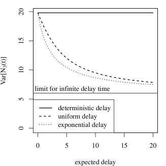
Figure 1: The results from Theorem 3.4, Lemma 4.1 and Lemma 4.2 are summarized in this figure. We fix $\lambda_{1}^{+}=\lambda_{1}^{-}=\lambda_{2}=\lambda_{3}=1$, $\tau_{1}=1,\tau_{2}=2,\tau_{3}=3$ here. We display the dependency of the variance of the number of proteins $\mathbf{Var}[\mathcal{N}_{3}(t)]$, on the expected delay time. For deterministic delay, the variance does not change in equilibrium, while it decreases for uniform and even more for exponentially distributed delay. For simplicity, we choose $b=d$ and $a=c=0$ for Lemma 4.1 and $\sigma_{2}=\sigma_{3}$ in Lemma 4.2.

4.1 Uniform delay

Lemma 4.1 (Uniform delay).

Let $\mu$ be the uniform distribution on $[a,b]$, $\nu$ be the uniform distribution on $[c,d]$ and $G_{2},G_{2}^{\prime}\sim\mu,G_{3},G_{3}^{\prime}\sim\nu$ be independent. Then, for $e_{+}:=max(d-c,b-a)$ and $e_{-}:=\min(d-c,b-a)$,

$$\mathbf{E}\Big{[}e^{-\frac{|G_{2}-G_{2}^{\prime}|}{\tau}}\Big{]} =\frac{2\tau}{b-a}\Big{(}1-\frac{\tau}{b-a}(1-e^{-\frac{b-a}{\tau}})\Big{)},$$

$$\mathbf{E}\Big{[}e^{-\frac{|G_{3}-G_{3}^{\prime}+G_{2}-G_{2}^{\prime}|}{\tau}}\Big{]} =\frac{2\tau}{3(b-a)^{2}(d-c)^{2}}\Big{(}3e_{-}^{2}e_{+}-e_{-}^{3}-6e_{-}\tau^{2}$$

$$\qquad\qquad\qquad\qquad+3e^{-\frac{e_{-}+e_{+}}{\tau}}(e^{\frac{e_{-}}{\tau}}-1)(e^{\frac{e_{-}}{\tau}}+2e^{\frac{e_{+}}{\tau}}-1)\tau^{3}\Big{)}.$$

Proof.

Without loss of generality we can assume that $a=c=0$ since deterministic delays do not affect our result. Let $G_{2},G_{2}^{\prime}\sim\mu$ and $G_{3},G_{3}^{\prime}\sim\nu$ be independent. Note that the density of $\mu\ast\nu\sim G_{2}+G_{3}$ is given by (recall $s\wedge t:=\min(s,t)$ and $s^{+}:=\max(s,0)$)

$$f(x) =\frac{1}{bd}\int_{0}^{x}1_{y\leq b}1_{x-y\leq d}dy=\frac{1}{bd}\int_{(x-d)^{+}}^{x\wedge b}dy=\frac{(x\wedge b)-(x-d)^{+}}{bd}$$

for $0\leq x\leq b+d$. We need to compute (using Mathematica), assuming $b\leq d$,

$$\mathbf{E}\Big{[}e^{-\frac{|G_{2}-G_{2}^{\prime}|}{\tau}}\Big{]}=\frac{2}{b^{2}}\int_{0}^{b}\int_{0}^{x}e^{\frac{y-x}{\tau}}dydx=\frac{2\tau}{b^{2}}\int_{0}^{b}1-e^{-\frac{x}{\tau}}dx$$

$$\qquad=\frac{2\tau}{b}\Big{(}1-\frac{\tau}{b}(1-e^{-\frac{b}{\tau}})\Big{)},$$

$$\mathbf{E}\Big{[}e^{-\frac{|G_{3}-G_{3}^{\prime}+G_{2}-G_{2}^{\prime}|}{\tau}}\Big{]}=\frac{2}{b^{2}d^{2}}\int_{0}^{b+d}\int_{0}^{x}e^{\frac{y-x}{\tau}}((x\wedge b)-(x-d)^{+})$$

$$\qquad\qquad\qquad\qquad\qquad\qquad\qquad\cdot((y\wedge b)-(y-d)^{+})dydx$$

$$=\frac{2}{b^{2}d^{2}}\Big{(}\int_{0}^{b}\int_{0}^{x}e^{\frac{y-x}{\tau}}xydydx+\int_{b}^{b+d}\int_{0}^{b}e^{\frac{y-x}{\tau}}bydy$$

$$\qquad\qquad+\int_{b}^{b+d}\int_{b}^{x}e^{\frac{y-x}{\tau}}b^{2}dydx-\int_{d}^{b+d}\int_{d}^{x}e^{\frac{y-x}{\tau}}b(y-d)dydx$$

$$\qquad\qquad-\int_{d}^{b+d}\int_{0}^{b}e^{\frac{y-x}{\tau}}(x-d)ydydx-\int_{d}^{b+d}\int_{b}^{x}e^{\frac{y-x}{\tau}}(x-d)bdydx$$

$$\qquad\qquad+\int_{d}^{b+d}\int_{d}^{x}e^{\frac{y-x}{\tau}}(x-d)(y-d)dydx\Big{)}$$

$$=\frac{2\tau}{3b^{2}d^{2}}\Big{(}3b^{2}d-b^{3}+-6b\tau^{2}+3e^{-\frac{b+d}{\tau}}(e^{\frac{b}{\tau}}-1)(e^{\frac{b}{\tau}}+2e^{\frac{d}{\tau}}-1)\tau^{3}\Big{)}.$$

∎

4.2 Exponential delay

Lemma 4.2 (Exponential delay).

For $\sigma_{2},\sigma_{3}>0$, let $\mu$ be the $\exp(1/\sigma_{2})$-distribution, $\nu$ be the $\exp(1/\sigma_{3})$-distribution and $G_{2},G_{2}^{\prime}\sim\mu,G_{3},G_{3}^{\prime}\sim\nu$ be independent. Then,

$$\mathbf{E}\Big{[}e^{-\frac{|G_{2}-G_{2}^{\prime}|}{\tau}}\Big{]} =\frac{\tau}{\sigma_{2}+\tau},$$

$$\mathbf{E}\Big{[}e^{-\frac{|G_{3}-G_{3}^{\prime}+G_{2}-G_{2}^{\prime}|}{\tau}}\Big{]} =\frac{\tau(\sigma_{2}\sigma_{3}+\tau(\sigma_{2}+\sigma_{3}))}{(\tau+\sigma_{2})(\tau+\sigma_{3})(\sigma_{2}+\sigma_{3})}.$$

Proof.

Note that the distribution of $|G_{2}-G_{2}^{\prime}|$ has the density

$$f(x)=\frac{2}{\sigma_{2}^{2}}\int_{x}^{\infty}e^{-\frac{y}{\sigma_{2}}}e^{-\frac{y-x}{\sigma_{2}}}dy=\frac{1}{\sigma_{2}}e^{-\frac{x}{\sigma_{2}}},$$

i.e. is again an $\exp(1/\sigma_{2})$-distribution. Hence,

$$\mathbf{E}\Big{[}e^{-\frac{|G_{2}-G^{\prime}_{2}|}{\tau}}\Big{]} =\frac{\tau}{\sigma_{2}+\tau}.$$

Moreover, we can use Lemma A.1 with $t=0$, $G=G_{2},G^{\prime}=G_{2}^{\prime}$, $T=G_{3},T^{\prime}=G_{3}^{\prime}$, $\sigma=\sigma_{3}$, in order to see that

$$\mathbf{E}\Big{[}e^{-\frac{|G_{2}-G^{\prime}_{2}+G_{3}-G_{3}^{\prime}|}{\tau}}\Big{]} =\frac{\tau}{\tau+\sigma_{3}}\frac{\tau\mathbf{E}\Big{[}e^{-\frac{|G_{2}-G^{\prime}_{2}|}{\tau}}\Big{]}-\sigma_{3}\mathbf{E}\Big{[}e^{-\frac{|G_{2}-G^{\prime}_{2}|}{\sigma_{3}}}\Big{]}}{\tau-\sigma_{3}}$$

$$=\frac{\tau}{\tau+\sigma_{3}}\frac{\tau^{2}(\sigma_{2}+\sigma_{3})-\sigma_{3}^{2}(\sigma_{2}+\tau)}{(\tau-\sigma_{3})(\sigma_{2}+\tau)(\sigma_{2}+\sigma_{3})}$$

$$=\frac{\tau(\sigma_{2}\sigma_{3}+\tau(\sigma_{2}+\sigma_{3}))}{(\tau+\sigma_{2})(\tau+\sigma_{3})(\sigma_{2}+\sigma_{3})}.$$

∎

4.3 Small variance

Delays can be the result of various mechanisms; see Barrio et al. (2006) and references therein for a list of possible mechanisms. Hence, by the central limit theorem, it is reasonable to assume that the delay distribution has a small variance. For this case, we obtain the following result.

Corollary 4.3.

Let $G_{2},G_{2}^{\prime}\sim\mu$ and $G_{3},G_{3}^{\prime}\sim\nu$ are independent, and such that $\mathbf{Var}[G_{2}],\mathbf{Var}[G_{3}]$ is small. Then, if

$$\delta_{2}:=\mathbf{E}[|G_{2}-\mathbf{E}[G_{2}]|^{3}],\qquad\delta_{3}:=\mathbf{E}[|G_{3}-\mathbf{E}[G_{3}]|^{3}],$$

it holds for $\delta_{2},\delta_{3}\to 0$ that

$$\mathbf{Var}[\mathcal{N}_{2}(t)] =\lambda_{1}^{+}\lambda_{2}\tau_{1}\tau_{2}+\lambda_{1}^{+}\lambda_{1}^{-}\lambda_{2}^{2}\tau_{1}^{2}\tau_{2}\frac{1}{\tau_{1}+\tau_{2}}\Big{(}1-\frac{2\mathbf{Var}[G_{2}]}{\tau_{1}\tau_{2}}\Big{)}+\mathcal{O}(\delta_{2}),$$

$$\mathbf{Var}[\mathcal{N}_{3}(t)] =\lambda_{1}^{+}\lambda_{2}\lambda_{3}\tau_{1}\tau_{2}\tau_{3}+\lambda_{1}^{+}\lambda_{2}\lambda_{3}^{2}\frac{\tau_{1}\tau_{2}^{2}\tau_{3}^{2}}{\tau_{2}+\tau_{3}}\Big{(}1-\frac{2\mathbf{Var}[G_{3}]}{\tau_{2}\tau_{3}}\Big{)}$$

$$\qquad+\lambda_{1}^{+}\lambda_{1}^{-}\lambda_{2}^{2}\lambda_{3}^{2}\tau_{1}^{3}\tau_{2}^{2}\tau_{3}^{2}\frac{\tau_{1}\tau_{2}+\tau_{1}\tau_{3}+\tau_{2}\tau_{3}-\mathbf{Var}[G_{2}+G_{3}]}{(\tau_{1}+\tau_{2})(\tau_{1}+\tau_{3})(\tau_{2}+\tau_{3})}+\mathcal{O}(\delta_{2},\delta_{3}).$$

Proof.

We write

$$\mathbf{E}\big{[}e^{-\frac{|G_{2}^{\prime}-G_{2}|}{\tau}}\big{]} =\mathbf{E}\Big{[}1-\frac{|G_{2}^{\prime}-G_{2}|}{\tau}+\frac{(G_{2}^{\prime}-G_{2})^{2}}{\tau^{2}}+\mathcal{O}\Big{(}|G_{2}^{\prime}-G_{2}|^{3}\Big{)}\Big{]}$$

$$=\mathbf{E}\Big{[}1-\frac{|G_{2}^{\prime}-G_{2}|}{\tau}+\mathcal{O}\Big{(}|G_{2}^{\prime}-G_{2}|^{3}\Big{)}\Big{]}+\frac{2\mathbf{Var}[G_{2}]}{\tau^{2}}.$$

Hence, the first result concerning $\mathbf{Var}[\mathcal{N}_{2}(t)]$ follows directly from Theorem 3.2. For the variance of proteins,

$$\mathbf{E}\Big{[} e^{-\frac{|G_{3}-G_{3}^{\prime}+G_{2}-G_{2}^{\prime}|}{\tau}}\Big{]}$$

$$=\mathbf{E}\Big{[}1-\frac{|G_{3}-G_{3}^{\prime}+G_{2}-G_{2}^{\prime}|}{\tau}+\frac{(G_{3}-G_{3}^{\prime}+G_{2}-G_{2}^{\prime})^{2}}{\tau^{2}}$$

$$\qquad\qquad\qquad\qquad\qquad\qquad\qquad\qquad+\mathcal{O}\Big{(}|G_{2}-G_{2}^{\prime}|^{3},|G_{3}-G_{3}^{\prime}|^{3}\Big{)}\Big{]}$$

$$=\mathbf{E}\Big{[}1-\frac{|G_{3}-G_{3}^{\prime}+G_{2}-G_{2}^{\prime}|}{\tau}\Big{]}+\frac{2(\mathbf{Var}[G_{2}]+\mathbf{Var}[G_{3}])}{\tau^{2}}+\mathcal{O}(\delta_{2},\delta_{3}).$$

So, denoting the values of $A$ and $B$ from (16) with deterministic $G_{2}$ and $G_{3}$ by $A_{0}$ and $B_{0}$, respectively (compare with Remark 3.5), (16) gives

$$A_{0}-A =\frac{2\mathbf{Var}[G_{3}]}{(\tau_{2}+\tau_{3})\tau_{3}},$$

$$B_{0}-B =\frac{\tau_{1}}{(\tau_{1}+\tau_{3})(\tau_{1}-\tau_{3})}\Big{(}\frac{2\mathbf{Var}[G_{2}+G_{3}]\tau_{1}}{(\tau_{1}+\tau_{2})\tau_{2}}-\frac{2\mathbf{Var}[G_{2}+G_{3}]\tau_{3}}{(\tau_{2}+\tau_{3})\tau_{2}}\Big{)}+\mathcal{O}(\delta_{2},\delta_{3})$$

$$=\frac{2\mathbf{Var}[G_{2}+G_{3}]\tau_{1}}{(\tau_{1}+\tau_{2})(\tau_{1}+\tau_{3})(\tau_{2}+\tau_{3})}+\mathcal{O}(\delta_{2},\delta_{3}).$$

Hence, if $\mathbf{Var}$ is the variance of $\mathcal{N}_{3}(t)$ for deterministic $G_{2},G_{3}$,

$$\mathbf{Var}[\mathcal{N}_{3}(t)] =\mathbf{Var}-2\Big{(}\lambda_{1}^{+}\lambda_{2}\lambda_{3}^{2}\tau_{1}\tau_{2}\tau_{3}\frac{\mathbf{Var}[G_{3}]}{\tau_{2}+\tau_{3}}$$

$$\qquad\qquad+\lambda_{1}^{+}\lambda_{1}^{-}\lambda_{2}^{2}\lambda_{3}^{2}\tau_{1}^{3}\tau_{2}^{2}\tau_{3}^{2}\frac{\mathbf{Var}[G_{2}+G_{3}]}{(\tau_{1}+\tau_{2})(\tau_{1}+\tau_{3})(\tau_{2}+\tau_{3})}\Big{)}+\mathcal{O}(\delta_{2},\delta_{3})$$

and the result follows. ∎

5 Discussion

Our main results, Theorems 3.2 and 3.4 give precise formulas on the first two moments of the number of RNA and protein in equilibrium for the delay model considered in (1). We show that the expectation is not influenced by the delay but the variance tends to be highest without delay. As seen in Theoren 3.2 the variance $\mathbf{Var}[\mathcal{N}_{2}(t)]$ can be decomposed into the sum of

• $\mathbf{E}[\mathbf{Var}[\mathcal{N}_{2}(t)|\mathcal{N}_{1}]]=\mathbf{E}[\mathcal{N}_{2}(t)]=\lambda_{1}^{+}\lambda_{2}\tau_{1}\tau_{2}$

• $\mathbf{Var}[\mathbf{E}[\mathcal{N}_{2}(t)|\mathcal{N}_{1}]]=\lambda_{1}^{+}\lambda_{1}^{-}\lambda_{2}^{2}\tau_{1}^{2}\tau_{2}^{2}\cdot C$

with $C$ seen from (10). Here the first term can be interpreted as individual RNA-part and the second term as noise due to gene-activation-part. A similar decomposition also holds for the variance of protein number into (compare with Bowsher and Swain, 2012)

• $\mathbf{E}[\mathbf{Var}[\mathcal{N}_{3}(t)|\mathcal{N}_{1},\mathcal{N}_{2}]]=\lambda_{1}^{+}\lambda_{2}\lambda_{3}\tau_{1}\tau_{2}\tau_{3}$

• $\mathbf{E}[\mathbf{Var}[\mathbf{E}[\mathcal{N}_{3}(t)|\mathcal{N}_{1},\mathcal{N}_{2}]|\mathcal{N}_{1}]]=\lambda_{1}^{+}\lambda_{2}\lambda_{3}^{2}\tau_{1}\tau_{2}\tau_{3}^{2}\cdot A$

• $\mathbf{Var}[\mathbf{E}[\mathcal{N}_{3}(t)|\mathcal{N}_{1}]]=\lambda_{1}^{+}\lambda_{1}^{-}\lambda_{2}^{2}\lambda_{3}^{2}\tau_{1}^{2}\tau_{2}^{2}\tau_{3}^{2}\cdot B$,

where $A$ and $B$ are described in (15) and (16), respectively. These parts mirror the contribution of individual protein-noise, individual RNA-noise and noise caused by gene activation to the variance in protein number, respectively. Such a variance decomposition is well-known for the model without delay (Paulsson, 2005) and is helpful in understanding the different kind of effects. Our results on this variance decomposition, togehter with the concrete formulas for $A$ and $B$ seem to be the first analytical solution of the delay model from (1) for gene expression.

It has been known for a long time that production of proteins (within a system of active and deactive genes) comes in bursts. Although our results on the first two moments give only a first impression about this burst-like behavior, the connection is only indirect. We rely on the intuition that a higher variance is compatible with a more burst-like behavior of protein. With this interpretation, we find that burst-like behavior is highest without delay. This result can also be explained intuitively: Delay weakens the discrete transitions between the state of gene or the number of RNA respectively. Consequently the RNA and protein expression patterns tend to be less bursty given delay.

Analytical approaches for biochemical systems frequently utilize the Master equation, available for any Markov process. Since delays lead to non-Markovian processes, this technique has to be adapted in order to capture delays. One way out – e.g. carried out in Bratsun et al. (2005) and Tian et al. (2007) – is to use independence of two-point probabilities in the Master equation in order to have a closed system of delay differential equations. However, note that the resulting description is not precise, whereas the model equations (2) provide an exact description of delay stochastic systems; compare also with the approach from Anderson (2007).

Delays have been considered for gene expression in equations for protein degradation and feedback in Bratsun et al. (2005) by lumping transcription and translation into a single process. Protein degradation is a process involving complex proteolytic pathways and a cellular degradation machinery, leading to several delays; see also Fromion et al. (2013). Moreover, transcription via elongation is known to produce delays which are able to explain oscillatory behavior of feedback systems (Monk, 2003; Roussel and Zhu, 2006b) Interestingly, Bratsun et al. (2005) find examples with feedback where the stochastic system is oscillatory even if the corresponding deterministic system is non-oscillatory. Such oscillatory behavior was also modeled for the expression levels of both RNA and protein of the Notch effector Hes1 by Barrio et al. (2006).

A large part of theoretical work on delay models is dealing with simulation schemes for delay stochastic equations; see the review by Ribeiro (2010). Bratsun et al. (2005) extend the classical SSA method of Gillespie (1977) (which ignores delay) by keeping a list of reactions, which were initiated but finish only later. Another approach is to allow for memory reactions and memory species as used in Tian (2013). According to Barrio et al. (2006), delay reactions must be decomposed into consuming and non-consuming reactions. The reactants in an unfinished nonconsuming reaction can already participate in a new reaction, while they cannot participate in a consuming reaction. (An example of the former is a new initiation of transcription by binding of RNA polymerase can happen although the last transcription is not finished yet.) In this sense, our model (1) uses consuming reactions. These simulation schemes have been improved by schemes using a smaller number of random variables by Cai (2007) and Anderson (2007). The latter approach uses the Poisson process representation of delay models, much in the spirit of our paper; compare with (2).

Today, it is known that variances of protein numbers for the expression of a multitude of genes is mainly based on RNA flucations (Bar-Even et al., 2006). Clearly, this variance in protein number is also affected by delays. Hence, we have to know the variances in delay times for practical purposes, if we want to compare theoretical and empirical fluctuations in protein numbers. On the empirical side, measurements of delay time variances will be most important for understanding delay on gene regulation. On the theoretical side, an important extension of our theory would be to incorporate self-regulatory mechanisms. Note that several authors found that delays in such systems can lead to oscillatory behavior or even more bursty behavior (Monk, 2003; Zavala and Marquez-Lago, 2014; Bratsun et al., 2005; Zavala and Marquez-Lago, 2014). Describing such feedbacks using point processes will be a more thorough understanding of delays in gene regulation.

Appendix

Appendix A A key lemma

Within this section, we summarize some frequently used computations in the following lemma.

Lemma A.1.

Let $T,T^{\prime}$ be independent exponentially distributed with expectation $\sigma$, and $G,G^{\prime}\geq 0$ be independent and identically distributed. Then, for $t\in\mathbb{R},\tau>0$

$$\mathbf{E}\Big{[}e^{-\frac{|t+T+G-T^{\prime}-G^{\prime}|}{\tau}}\Big{]}=\frac{\tau}{\tau+\sigma}\frac{\tau\mathbf{E}\Big{[}e^{-\frac{|G^{\prime}-G-t|}{\tau}}\Big{]}-\sigma\mathbf{E}\Big{[}e^{-\frac{|G^{\prime}-G-t|}{\sigma}}\Big{]}}{\tau-\sigma}.$$ (20)

Moreover, if $$S S\stackrel{{\scriptstyle d}}{{=}}-S$$ has a symmetric distribution, i.e. ,

$$\mathbf{E}\Big{[}e^{-\frac{||T+G-T^{\prime}-G^{\prime}|-S|}{\tau}}\Big{]}=\mathbf{E}\Big{[}e^{-\frac{|T+G-T^{\prime}-G^{\prime}+S|}{\tau}}\Big{]}$$ (21)

$$\qquad\qquad\qquad\qquad\qquad=\frac{\tau}{\tau+\sigma}\frac{\tau\mathbf{E}\Big{[}e^{-\frac{|G^{\prime}-G+S|}{\tau}}\Big{]}-\sigma\mathbf{E}\Big{[}e^{-\frac{|G^{\prime}-G+S|}{\sigma}}\Big{]}}{\tau-\sigma}.$$

Remark A.2.

Note that in (20) and (21) all left hand sides include the exponentially distributed random variables $T,T^{\prime}$, while the right hand sides only depend on the distribution of $G,G^{\prime}$ (and $S$).

Proof.

We start with the proof of (20). First,

$$\mathbf{E}\Big{[} e^{-\frac{|t+T+G-T^{\prime}-G^{\prime}|}{\tau}}\Big{]}=\mathbf{E}\Big{[}\mathbf{E}\big{[}e^{-\frac{t+T+G-T^{\prime}-G^{\prime}}{\tau}}1_{T>T^{\prime}+G^{\prime}-G-t}\big{|}G-G^{\prime}\big{]}\Big{]}$$ (22)

$$\qquad\qquad\qquad\qquad\qquad+\mathbf{E}\Big{[}\mathbf{E}\big{[}e^{-\frac{T^{\prime}+G^{\prime}-T-G-t}{\tau}}1_{T^{\prime}\geq T+G-G^{\prime}+t}\big{|}G-G^{\prime}\big{]}\Big{]}$$

Then,

$$\mathbf{E} \big{[}e^{-\frac{t+T+G-T^{\prime}-G^{\prime}}{\tau}}1_{T>T^{\prime}+G^{\prime}-G-t}\big{|}G-G^{\prime}\big{]}$$ (23)

$$=1_{G^{\prime}-G-t\geq 0}\mathbf{E}\big{[}e^{-\frac{t+T+G-T^{\prime}-G^{\prime}}{\tau}}1_{T>T^{\prime}+G^{\prime}-G-t}\big{|}G-G^{\prime}\big{]}$$

$$\qquad\qquad\qquad+1_{G^{\prime}-G-t<0}\mathbf{E}\big{[}e^{-\frac{t+T+G-T^{\prime}-G^{\prime}}{\tau}}\big{(}1_{T^{\prime}<G-G^{\prime}+t}$$

$$\qquad\qquad\qquad\qquad\qquad\qquad\qquad+1_{T^{\prime}\geq G-G^{\prime}+t}1_{T>T^{\prime}+G^{\prime}-G-t}\big{)}\big{|}G-G^{\prime}\big{]}.$$

Now, on the set $\{G^{\prime}-G-t\geq 0\}$,

$$\mathbf{E}\big{[} e^{-\frac{t+T+G-T^{\prime}-G^{\prime}}{\tau}}1_{T>T^{\prime}+G^{\prime}-G-t}\big{|}G-G^{\prime}\big{]}=\frac{1}{2}e^{-\frac{G^{\prime}-G-t}{\sigma}}\mathbf{E}\big{[}e^{-\frac{T}{\tau}}\big{]}$$

$$=\frac{1}{2}\frac{\tau}{\sigma+\tau}e^{-\frac{G^{\prime}-G-t}{\sigma}}$$

since $\mathbf{P}[T>T^{\prime}+G^{\prime}-G-t|G-G^{\prime}]=\tfrac{1}{2}e^{-\frac{G^{\prime}-G-t}{\sigma}}$ and given $T>T^{\prime}+G^{\prime}-G-t$ and conditioned on $G-G^{\prime}$, the random variable $t+T+G-T^{\prime}-G^{\prime}$ is again exponentially distributed with expectation $\sigma$. Next, on $\{G^{\prime}-G-t<0\}$

$$\mathbf{E}\big{[}e^{-\frac{t+T+G-T^{\prime}-G^{\prime}}{\tau}} 1_{T^{\prime}<G-G^{\prime}+t}\big{|}G-G^{\prime}\big{]}$$

$$=\int_{0}^{\infty}\int_{0}^{G-G^{\prime}+t}\frac{1}{\sigma^{2}}e^{-\frac{s^{\prime}+s}{\sigma}}e^{-\frac{t+s+G-s^{\prime}-G^{\prime}}{\tau}}ds^{\prime}ds$$

$$=\frac{1}{\sigma^{2}}e^{-\frac{G-G^{\prime}+t}{\tau}}\int_{0}^{\infty}e^{-s\big{(}\frac{1}{\sigma}+\frac{1}{\tau}\big{)}}ds\int_{0}^{G-G^{\prime}+t}e^{-s^{\prime}\big{(}\frac{1}{\sigma}-\frac{1}{\tau}\big{)}}ds^{\prime}$$

$$=\frac{1/\sigma}{1/\sigma+1/\tau}\frac{1/\sigma}{1/\sigma-1/\tau}e^{-\frac{G-G^{\prime}+t}{\tau}}\big{(}1-e^{-(G-G^{\prime}+t)\big{(}\frac{1}{\sigma}-\frac{1}{\tau}\big{)}}\big{)}$$

$$=\frac{\tau^{2}}{(\tau+\sigma)(\tau-\sigma)}\big{(}e^{-\frac{G-G^{\prime}+t}{\tau}}-e^{-\frac{G-G^{\prime}+t}{\sigma}}\big{)}$$

as well as

$$\mathbf{E} \big{[}e^{-\frac{t+T+G-T^{\prime}-G^{\prime}}{\tau}}1_{T^{\prime}\geq G-G^{\prime}+t}1_{T>T^{\prime}+G^{\prime}-G-t}\big{|}G-G^{\prime}\big{]}$$

$$=e^{-\frac{t+G-G^{\prime}}{\sigma}}\mathbf{E}\big{[}e^{-\frac{T-T^{\prime}}{\tau}}1_{T>T^{\prime}}|G-G^{\prime}\big{]}=\frac{1}{2}e^{-\frac{t+G-G^{\prime}}{\sigma}}\frac{\tau}{\sigma+\tau}$$

since $\mathbf{P}[T^{\prime}>G-G^{\prime}+t|G-G^{\prime}]=e^{-\frac{t+G-G^{\prime}}{\sigma}}$ and given $T^{\prime}>G-G^{\prime}+t$, the random variable $T^{\prime}+G^{\prime}-G-t$ is again exp$(\sigma)$ distributed. Plugging the last three computations into (23),

$$\mathbf{E} \big{[}e^{-\frac{t+T+G-T^{\prime}-G^{\prime}}{\tau}}1_{T>T^{\prime}+G^{\prime}-G-t}\big{|}G-G^{\prime}\big{]}$$

$$=\frac{1}{2}\frac{\tau}{\sigma+\tau}e^{-\frac{|G^{\prime}-G-t|}{\tau}}+1_{G^{\prime}-G-t<0}\frac{\tau^{2}}{(\tau+\sigma)(\tau-\sigma)}\big{(}e^{-\frac{G-G^{\prime}+t}{\tau}}-e^{-\frac{G-G^{\prime}+t}{\sigma}}\big{)}.$$

Then, by symmetry of $G-G^{\prime}$, from (22),

$$\mathbf{E} \big{[}e^{-\frac{|t+T+G-T^{\prime}-G^{\prime}|}{\tau}}\big{]}$$

$$=\mathbf{E}\Big{[}\frac{1}{2}\frac{\tau}{\sigma+\tau}e^{-\frac{|G^{\prime}-G-t|}{\sigma}}+1_{G^{\prime}-G-t<0}\frac{\tau^{2}}{(\tau+\sigma)(\tau-\sigma)}\big{(}e^{-\frac{G-G^{\prime}+t}{\tau}}-e^{-\frac{G-G^{\prime}+t}{\sigma}}\big{)}\Big{]}$$

$$\quad+\mathbf{E}\Big{[}\frac{1}{2}\frac{\tau}{\sigma+\tau}e^{-\frac{|G-G^{\prime}+t|}{\sigma}}+1_{G-G^{\prime}+t<0}\frac{\tau^{2}}{(\tau+\sigma)(\tau-\sigma)}\big{(}e^{-\frac{G^{\prime}-G-t}{\tau}}-e^{-\frac{G^{\prime}-G-t}{\sigma}}\big{)}\Big{]}$$

$$=\frac{\tau}{\sigma+\tau}\mathbf{E}\Big{[}e^{-\frac{|G^{\prime}-G-t|}{\sigma}}\Big{]}+\frac{\tau^{2}}{(\tau+\sigma)(\tau-\sigma)}\mathbf{E}\Big{[}e^{-\frac{|G^{\prime}-G-t|}{\tau}}-e^{-\frac{|G^{\prime}-G-t|}{\sigma}}\Big{]}$$

$$=\frac{\tau}{\tau+\sigma}\frac{\tau\mathbf{E}\Big{[}e^{-\frac{|G^{\prime}-G-t|}{\tau}}\Big{]}-\sigma\mathbf{E}\Big{[}e^{-\frac{|G^{\prime}-G-t|}{\sigma}}\Big{]}}{\tau-\sigma}.$$

For, (21), we only need to show the first equality since the second follows from (20) by conditioning on $S$. Using the symmetry of $S$ we can write

$$\mathbf{E}\Big{[}e^{-\frac{||T+G-T^{\prime}-G^{\prime}|-S|}{\tau}}\Big{]} =\mathbf{E}\Big{[}e^{-\frac{|T+G-T^{\prime}-G^{\prime}-S|}{\tau}},T+G-T^{\prime}-G^{\prime}\geq 0\Big{]}$$

$$\qquad\qquad\qquad+\mathbf{E}\Big{[}e^{-\frac{|T^{\prime}+G^{\prime}-T-G+S|}{\tau}},T+G-T^{\prime}-G^{\prime}<0\Big{]}$$

$$=\mathbf{E}\Big{[}e^{-\frac{|T+G-T^{\prime}-G^{\prime}-S|}{\tau}}\Big{]}$$

which shows the first equality in (21). ∎

Acknowledgments

We thank Bence Melykuti for helpful comments on the manuscript.

References

• A and van Oudenaarden (2008) A, A. R. and A. van Oudenaarden (2008). Nature, nurture, or chance: Stochastic gene expression and its consequences. Cell 135, 216–226.
• Anderson (2007) Anderson, D. (2007). A modified next reaction method for simulating chemical systems with time dependent propensities and delays. J. Chem. Phys. 127(21), 214107–214107.
• Anderson and Kurtz (2011) Anderson, D. and T. G. Kurtz (2011). Continuous time Markov chain models for chemical reaction networks. In Design and Analysis of Biomolecular Circuits: Engineering Approaches to Systems and Synthetic Biology. Springer.
• Balazsi et al. (2011) Balazsi, G., A. van Oudenaarden, and J. J. Collins (2011). Cellular decision making and biological noise: from microbes to mammals. Cell 144, 910–925.
• Bar-Even et al. (2006) Bar-Even, A., J. Paulsson, N. Maheshri, M. Carmi, E. O’Shea, Y. Pilpel, and N. Barkai (2006). Noise in protein expression scales with natural protein abundance. Nature Genetics 38, 636–643.
• Barrio et al. (2006) Barrio, M., K. Burrage, A. Leier, and T. T. Tian (2006). Oscillatory regulation of hes1: Discrete stochastic delay modelling and simulation. PLoS Comput. Biol. 2(9), e117.
• Barrio et al. (2013) Barrio, M., A. Leier, and T. T. Marquez-Lago (2013). Reduction of chemical reaction networks through delay distributions. J. Chem. Phys. 138(10), 104114–104114.
• Berg (1978) Berg, O. G. (1978). A model for statistical fluctuations of protein numbers in a microbial-population. J. Theor. Biol. 71, 587–603.
• Bokes et al. (2012) Bokes, P., J. R. King, A. T. A. Wood, and M. Loose (2012). Exact and approximate distributions of protein and mrna levels in the low-copy regime of gene expression. J. Math. Biol. 64, 829–854.
• Bowsher and Swain (2012) Bowsher, C. G. and P. S. Swain (2012). Identifying sources of variation and the flow of information in biochemical networks. Proceedings of the National Academy of Sciences 109(20), E1320–E1328.
• Bratsun et al. (2005) Bratsun, D., D. Volfson, L. S. Tsimring, and J. Hasty (2005). Delay-induced stochastic oscillations in gene regulation. Proc. Natl. Acad. Sci. USA 102(41), 14593–14598.
• Cai (2007) Cai, X. (2007). Exact stochastic simulation of coupled chemical reactions with delays. J. Chem. Phys. 126(12), 124108–124108.
• Cottrell et al. (2012) Cottrell, D., P. S. Swain, and P. F. Tupper (2012). Stochastic branching-diffusion models for gene expression. Proc. Natl. Acad. Sci. USA 109(25), 9699–9704.
• Fromion et al. (2013) Fromion, V., E. Leoncini, and P. Robert (2013). Stochastic gene expression in cells: A point process approach. SIAM J. Appl. Math. 73(1), 195–211.
• Gillespie (1977) Gillespie, D. (1977). Exact stochastic simulation of coupled chemical reactions. J. Phys. Chem. 81, 2340–2361.
• Gillespie et al. (2013) Gillespie, D., A. Hellander, and L. Petzold (2013). Perspective: Stochastic algorithms for chemical kinetics. J. Chem. Phys. 138, 170901.
• Guptasarma (1995) Guptasarma, P. (1995). Does replication-induced transcription regulate synthesis of the myriad low copy number proteins of escherichia coli? Bioessays 17(11), 987–997.
• Iyer-Biswas et al. (2009) Iyer-Biswas, S., F. Hayot, and C. Jayaprakash (2009). Stochasticity of gene products from transcriptional pulsing. Phys. Rev. E Stat. Nonlin. Soft Matter Phys. 79(3 Pt 1), 031911–031911.
• Jackson et al. (2000) Jackson, D. A., A. N. A. Pombo, and F. Iborra (2000). The balance sheet for transcription: an analysis of nuclear rna metabolism in mammalian cells. The FASEB Journal 14(2), 242–254.
• Kaern et al. (2005) Kaern, M., T. C. Elston, W. J. Blake, and J. J. Collins (2005). Stochasticity in gene expression: from theories to phenotypes. Nat. Rev. Genet. 6(6), 451–464.
• Kærn et al. (2005) Kærn, M., T. C. Elston, W. J. Blake, and J. J. Collins (2005). Stochasticity in gene expression: from theories to phenotypes. Nature Reviews Genetics 6(6), 451–464.
• Leier et al. (2014) Leier, A., M. Barrio, and T. Marquez-Lago (2014). Exact model reduction with delays: closed-form distributions and extensions to fully bi-directional monomolecular reactions. Interface 11, 20140108.
• Lewis (2003) Lewis, J. (2003). Autoinhibition with transcriptional delay: a simple mechanism for the zebrafish somitogenesis oscillator. Curr. Biol. 13(16), 1398–1408.
• McAdams and Arkin (1997) McAdams, H. H. and A. Arkin (1997). Stochastic mechanisms in gene expression. Proc. Natl. Acad. Sci. USA 94(3), 814–819.
• Monk (2003) Monk, N. A. (2003). Oscillatory expression of Hes1, p53, and NF-kappaB driven by transcriptional time delays. Curr. Biol. 13(16), 1409–1413.
• Paulsson (2005) Paulsson, J. (2005). Models of stochastic gene expression. Physics of Life Review 2, 157–175.
• Pendar et al. (2013) Pendar, H., T. Platini, and R. V. Kulkarni (2013). Exact protein distributions for stochastic models of gene expression using partitioning of poisson processes. Phys. Rev. E 87, 042720.
• Raj and ”van Oudenaarden” (2008) Raj, A. and A. ”van Oudenaarden” (2008). Nature, nurture, or chance: stochastic gene expression and its consequences. Cell 135(2), 216–226.
• Raser and O’Shea (2005) Raser, J. M. and E. K. O’Shea (2005). Noise in gene expression: origins, consequences, and control. Science 309, 2010–2013.
• Ribeiro (2010) Ribeiro, A. S. (2010). Stochastic and delayed stochastic models of gene expression and regulation. Math. Biosci. 223(1), 1–11.
• Rigney and Schieve (1977) Rigney, D. R. and W. C. Schieve (1977). Stochastic model of linear, continuous protein synthesis in bacterial populations. J. Theor. Biol. 69(4), 761–766.
• Roussel (1996) Roussel, M. R. (1996). The use of delay differential equations in chemical kinetics. J. Phys. Chem. 100, 8323––8330.
• Roussel and Zhu (2006a) Roussel, M. R. and R. Zhu (2006a). Stochastic kinetics description of a simple transcription model. Bull. Math. Biol. 68(7), 1681–1713.
• Roussel and Zhu (2006b) Roussel, M. R. and R. Zhu (2006b). Validation of an algorithm for delay stochastic simulation of transcription and translation in prokaryotic gene expression. Phys. Biol. 3(4), 274–284.
• Swain et al. (2002) Swain, P. S., M. B. Elowitz, and E. D. Siggia (2002). Intrinsic and extrinsic contributions to stochasticity in gene expression. Proc. Natl. Acad. Sci. USA 99(20), 12795–12800.
• Tian (2013) Tian, T. (2013). Chemical memory reactions induced bursting dynamics in gene expression. PLoS One 8(1), e52029.
• Tian et al. (2007) Tian, T., K. Burrage, P. M. Burrage, and M. Carletti (2007). Stochastic delay differential equations for genetic regulatory networks. Journal of Computational and Applied Mathematics 205, 696–707.
• Zavala and Marquez-Lago (2014) Zavala, E. and T. T. Marquez-Lago (2014). Delays induce novel stochastic effects in negative feedback gene circuits. Biophysical journal 106(2), 467–478.
• Zhu et al. (2007) Zhu, R., A. S. Ribeiro, D. Salahub, and S. A. Kauffman (2007). Studying genetic regulatory networks at the molecular level: delayed reaction stochastic models. J. Theor. Biol. 246(4), 725–745.
• Zhu and Salahub (2008) Zhu, R. and D. Salahub (2008). Delay stochastic simulation of single-gene expression reveals a detailed relationship between protein noise and mean abundance. FEBS Lett. 582(19), 2905–2910.