User Guide for the Discrete Dipole
Approximation Code DDSCAT 7.3

Abstract

DDSCAT 7.3 is a freely available open-source Fortran-90 software package applying the “discrete dipole approximation” (DDA) to calculate scattering and absorption of electromagnetic waves by targets with arbitrary geometries and complex refractive index. The targets may be isolated entities (e.g., dust particles), but may also be 1-d or 2-d periodic arrays of “target unit cells”, which can be used to study absorption, scattering, and electric fields around arrays of nanostructures.

The DDA approximates the target by an array of polarizable points. The theory of the DDA and its implementation in DDSCAT is presented in Draine (1988) and Draine & Flatau (1994), and its extension to periodic structures in Draine & Flatau (2008). Efficient near-field calculations are carried out as described in Flatau & Draine (2012). DDSCAT 7.3 allows accurate calculations of electromagnetic scattering from targets with “size parameters” $2\pi{a}_{\rm eff}/\lambda\lower 2.15277pt\hbox{$\;\buildrel<\over{\sim}\;$}25$ provided the refractive index $m$ is not large compared to unity ($|m-1|\lower 2.15277pt\hbox{$\;\buildrel<\over{\sim}\;$}2$). DDSCAT 7.3 includes support for MPI, OpenMP, and the Intel^® Math Kernel Library (MKL).

DDSCAT supports calculations for a variety of target geometries (e.g., ellipsoids, regular tetrahedra, rectangular solids, finite cylinders, hexagonal prisms, etc.). Target materials may be both inhomogeneous and anisotropic. It is straightforward for the user to “import” arbitrary target geometries into the code. DDSCAT automatically calculates total cross sections for absorption and scattering and selected elements of the Mueller scattering intensity matrix for specified orientation of the target relative to the incident wave, and for specified scattering directions. DDSCAT 7.3 can calculate scattering and absorption by targets that are periodic in one or two dimensions. DDSCAT 7.3 can calculate and store ${\bf E}$ and ${\bf B}$ throughout a user-specified rectangular volume containing the target. A Fortran-90 code ddpostprocess to support postprocessing of ${\bf P}$, and nearfield ${\bf E}$ and ${\bf B}$, is included in the distribution.

DDSCAT 7.3 differs from DDSCAT 7.2 by offering two new options: (1) The “Filtered Coupled Dipole” method (Piller & Martin 1998; Gay-Balmaz & Martin 2002) for DDA calculations. (2) Fast near-field calculations of ${\bf B}$. In addition, a new postprocessing code DDPOSTPROCESS.f90 is provided that is well-documented, and much more easily modifiable by the user. As distributed, ddpostprocess calculates the Poynting vector.

This User Guide explains how to use DDSCAT 7.3 (release 7.3.0) to carry out electromagnetic scattering calculations. If you publish results calculated using DDSCAT 7.3, please cite relevant publications describing the methods, e.g., Draine & Flatau (1994), Draine & Flatau (2008), and Flatau & Draine (2012).

1 Introduction

DDSCAT is a software package to calculate scattering and absorption of electromagnetic waves by targets with arbitrary geometries using the “discrete dipole approximation” (DDA). In this approximation the target is replaced by an array of point dipoles (or, more precisely, polarizable points); the electromagnetic scattering problem for an incident periodic wave interacting with this array of point dipoles is then solved essentially exactly. The DDA (sometimes referred to as the “coupled dipole approximation”) was apparently first proposed by Purcell & Pennypacker (1973). DDA theory was reviewed and developed further by Draine (1988), Draine & Goodman (1993), reviewed by Draine & Flatau (1994), and recently extended to periodic structures by Draine & Flatau (2008).

DDSCAT 7.3, the current release of DDSCAT, is an open-source Fortran 90 implementation of the DDA developed by the authors. DDSCAT 7.3 calculates absorption and scattering by isolated targets, or targets that are periodic in one or two dimensions, using methods described by Draine & Flatau (2008).

DDSCAT is intended to be a versatile tool, suitable for a wide variety of applications including studies of interstellar dust, atmospheric aerosols, blood cells, marine microorganisms, and nanostructure arrays. As provided, DDSCAT 7.3 should be usable for many applications without modification, but the program is written in a modular form, so that modifications, if required, should be fairly straightforward.

The authors make this code openly available to others, in the hope that it will prove a useful tool. We ask only that:

• If you publish results obtained using DDSCAT, please acknowledge the source of the code, and cite relevant papers, such as Draine (1988), Goodman et al. (1990), Draine & Flatau (1994), Draine & Flatau (2008), and Flatau & Draine (2012).

• If you discover any errors in the code or documentation, please promptly communicate them to the authors.

• You comply with the “copyleft" agreement (more formally, the GNU General Public License) of the Free Software Foundation: you may copy, distribute, and/or modify the software identified as coming under this agreement. If you distribute copies of this software, you must give the recipients all the rights which you have. See the file doc/copyleft.txt distributed with the DDSCAT software.

We also strongly encourage you to send email to draine@astro.princeton.edu identifying yourself as a user of DDSCAT; this will enable the authors to notify you of any bugs, corrections, or improvements in DDSCAT. Up-to-date information on DDSCAT and the latest version of DDSCAT 7.3 can be found at
      http://code.google.com/p/ddscat/

The current version, DDSCAT 7.3, offers the option of using the DDA formulae from Draine (1988), with dipole polarizabilities determined from the Lattice Dispersion Relation (Draine & Goodman 1993; Gutkowicz-Krusin & Draine 2004). Alternatively, DDSCAT 7.3 also allows the user to specify the “filtered coupled dipole” method of Piller & Martin (1998) and Gay-Balmaz & Martin (2002), which may give better results for targets with “large” refractive indices $|m-1|\lower 2.15277pt\hbox{$\;\buildrel>\over{\sim}\;$}2$.

The code incorporates Fast Fourier Transform (FFT) methods (Goodman et al. 1990). DDSCAT 7.3 includes capability to calculate scattering and absorption by targets that are periodic in one or two dimensions – arrays of nanostructures, for example. The theoretical basis for application of the DDA to periodic structures is developed in Draine & Flatau (2008). DDSCAT 7.3 includes capability to efficiently perform “nearfield” calculations of ${\bf E}$ and ${\bf B}$ in and around the target using FFT methods, as described by Flatau & Draine (2012). A new postprocessing code, DDPOSTPROCESS.f90, is included in the DDSCAT 7.3 distribution.

We refer you to the list of references at the end of this document for discussions of the theory and accuracy of the DDA [in particular, reviews by Draine & Flatau (1994) and Draine (2000), recent extension to 1-d and 2-d arrays by Draine & Flatau (2008), and comparison of the coupled dipole method with other DDA methods (including the filtered coupled dipole method) by Yurkin et al. (2010)].

In §2 we summarize the applicability of the DDA, and in §3 we describe what the current release can calculate.

In §4 we describe the principal changes between DDSCAT 7.3 and the previous releases. The succeeding sections contain instructions for:

• obtaining the source code (§5);

• compiling and linking the code (§6);

• information for Microsoft^® Windows users (§7);

• running a sample calculation (§8);

• modifying the parameter file to do your desired calculations (§9);

• specifying target orientation(s) (§19);

• understanding the output from the sample calculation;

• using DDPOSTPROCESS.f90 for postprocessing of solutions found by DDSCAT 7.3 (§30.1).

The instructions for compiling, linking, and running will be appropriate for a Linux system; slight changes will be necessary for non-Linux sites, but they are quite minor and should present no difficulty.

Finally, the current version of this User Guide can be obtained from
http://arxiv.org/abs/xxxx.xxxx.

Important Note: DDSCAT 7.3 differs in a number of respects from previous versions of DDSCAT. DDSCAT 7.3 includes support for both MPI and OpenMP, but – as of this writing – DDSCAT 7.3 has not yet been tested with MPI, and there has been only limited testing with OpenMP. DDSCAT 7.3 has been tested extensively on single-processor systems, but if you are intending to use DDSCAT 7.3 with OpenMP or MPI, please proceed with caution – do at least a few comparison calculations in single-cpu mode to verify that the results obtained with OpenMP or MPI appear to be correct. If you do encounter problems with OpenMP or MPI, please document them and communicate them to the authors. And if you find that everything appears to work properly, we’d like to know that too!

2 Applicability of the DDA

The principal advantage of the DDA is that it is completely flexible regarding the geometry of the target, being limited only by the need to use an interdipole separation $d$ small compared to (1) any structural lengths in the target, and (2) the wavelength $\lambda$. Numerical studies (Draine & Goodman 1993; Draine & Flatau 1994; Draine 2000) indicate that the second criterion is adequately satisfied if

$$|m|kd<1\leavevmode\nobreak\ \leavevmode\nobreak\ \leavevmode\nobreak\ ,$$ (1)

where $m$ is the complex refractive index of the target material, and $k\equiv 2\pi/\lambda$, where $\lambda$ is the wavelength in vacuo. This criterion is valid provided that $|m-1|\lower 2.15277pt\hbox{$\;\buildrel<\over{\sim}\;$}3$ or so. When Im$(m)$ becomes large, the DDA solution tends to overestimate the absorption cross section $C_{\rm abs}$, and it may be necessary to use interdipole separations $d$ smaller than indicated by eq. (1) to reduce the errors in $C_{\rm abs}$ to acceptable values.

If accurate calculations of the scattering phase function (e.g., radar or lidar cross sections) are desired, a more conservative criterion

$$|m|kd<0.5$$ (2)

will usually ensure that differential scattering cross sections $dC_{\rm sca}/d\Omega$ are accurate to within a few percent of the average differential scattering cross section $C_{\rm sca}/4\pi$ (see Draine 2000).

Let $V$ be the actual volume of solid material in the target. If the target is represented by an array of $N$ dipoles, located on a cubic lattice with lattice spacing $d$, then

$$V=Nd^{3}\leavevmode\nobreak\ \leavevmode\nobreak\ \leavevmode\nobreak\ .$$ (3)

We characterize the size of the target by the “effective radius”

$$a_{\rm eff}\equiv(3V/4\pi)^{1/3}\leavevmode\nobreak\ \leavevmode\nobreak\ \leavevmode\nobreak\ ,$$ (4)

the radius of an equal volume sphere. A given scattering problem is then characterized by the dimensionless “size parameter”

$$x\equiv ka_{\rm eff}=\frac{2\pi a_{\rm eff}}{\lambda}\leavevmode\nobreak\ \leavevmode\nobreak\ \leavevmode\nobreak\ .$$ (5)

The size parameter can be related to $N$ and $|m|kd$:

$$x\equiv{2\pi a_{\rm eff}\over\lambda}={62.04\over|m|}\left({N\over 10^{6}}\right)^{1/3}\cdot|m|kd\leavevmode\nobreak\ \leavevmode\nobreak\ \leavevmode\nobreak\ .$$ (6)

Equivalently, the target size can be written

$$a_{\rm eff}=9.873{\lambda\over|m|}\left({N\over 10^{6}}\right)^{1/3}\cdot|m|kd\leavevmode\nobreak\ \leavevmode\nobreak\ \leavevmode\nobreak\ .$$ (7)

Practical considerations of CPU speed and computer memory currently available on scientific workstations typically limit the number of dipoles employed to $N<10^{6}$ (see §17 for limitations on $N$ due to available RAM); for a given $N$, the limitations on $|m|kd$ translate into limitations on the ratio of target size to wavelength.

For calculations of total cross sections $C_{\rm abs}$ and $C_{\rm sca}$, we require $|m|kd<1$:

$$a_{\rm eff}<9.88{\lambda\over|m|}\left({N\over 10^{6}}\right)^{1/3}{\rm\leavevmode\nobreak\ \leavevmode\nobreak\ or\leavevmode\nobreak\ \leavevmode\nobreak\ }x<{62.04\over|m|}\left({N\over 10^{6}}\right)^{1/3}\leavevmode\nobreak\ \leavevmode\nobreak\ \leavevmode\nobreak\ .$$ (8)

For scattering phase function calculations, we require $|m|kd<0.5$:

$$a_{\rm eff}<4.94{\lambda\over|m|}\left({N\over 10^{6}}\right)^{1/3}{\rm\leavevmode\nobreak\ \leavevmode\nobreak\ \leavevmode\nobreak\ \leavevmode\nobreak\ or\leavevmode\nobreak\ \leavevmode\nobreak\ \leavevmode\nobreak\ \leavevmode\nobreak\ }x<{31.02\over|m|}\left({N\over 10^{6}}\right)^{1/3}\leavevmode\nobreak\ \leavevmode\nobreak\ \leavevmode\nobreak\ .$$ (9)

It is therefore clear that the DDA is not suitable for very large values of the size parameter $x$, or very large values of the refractive index $m$. The primary utility of the DDA is for scattering by dielectric targets with sizes comparable to the wavelength. As discussed by Draine & Goodman (1993), Draine & Flatau (1994), and Draine (2000), total cross sections calculated with the DDA are accurate to a few percent provided $N>10^{4}$ dipoles are used, criterion (1) is satisfied, and the refractive index is not too large.

For fixed $|m|kd$, the accuracy of the approximation degrades with increasing $|m-1|$, for reasons having to do with the surface polarization of the target, as discussed by Collinge & Draine (2004). With the present code, good accuracy can be achieved for $|m-1|<2$.

Figure 1: Scattering and absorption for a sphere with $m=1.33+0.01i$. The upper panel shows the exact values of $Q_{\rm sca}$ and $Q_{\rm abs}$, obtained with Mie theory, as functions of $x=ka$. The middle and lower panels show fractional errors in $Q_{\rm sca}$ and $Q_{\rm abs}$, obtained using DDSCAT with polarizabilities obtained from the Lattice Dispersion Relation, and labelled by the number $N$ of dipoles in each pseudosphere. After Fig. 1 of Draine & Flatau (1994).

Figure 2: Same as Fig. 1, but for $m=2+i$. After Fig. 2 of Draine & Flatau (1994). Note: in the upper panel, the labels for $Q_{\rm sca,Mie}$ and $Q_{\rm abs,Mie}$ should be interchanged.

Figure 3: Differential scattering cross section for $m=1.33+0.01i$ pseudosphere and $ka=7$. Lower panel shows fractional error compared to exact Mie theory result. The $N=17904$ pseudosphere has $|m|kd=0.57$, and an rms fractional error in $d\sigma/d\Omega$ of 2.4%. After Fig. 5 of Draine & Flatau (1994).

Figure 4: Same as Fig. 3 but for $m=2+i$. The $N=59728$ pseudosphere has $|m|kd=0.65$, and an rms fractional error in $d\sigma/d\Omega$ of 6.7%. After Fig. 8 of Draine & Flatau (1994).

Examples illustrating the accuracy of the DDA are shown in Figs. 1–2, which show overall scattering and absorption efficiencies as a function of wavelength for different discrete dipole approximations to a sphere, with $N$ ranging from 304 to 59728. The DDA calculations assumed radiation incident along the (1,1,1) direction in the “target frame”. Figs. 3–4 show the scattering properties calculated with the DDA for $x=ka=7$. Additional examples can be found in Draine & Flatau (1994) and Draine (2000).

As discussed below, DDSCAT 7.3 can also calculate scattering and absorption by targets that are periodic in one or two directions – for examples, see Draine & Flatau (2008).

3 DDSCAT 7.3

3.1 What Does It Calculate?

3.1.1 Absorption and Scattering by Finite Targets

DDSCAT 7.3, like previous versions of DDSCAT, solves the problem of scattering and absorption by a finite target, represented by an array of polarizable point dipoles, interacting with a monochromatic plane wave incident from infinity. DDSCAT 7.3 has the capability of automatically generating dipole array representations for a variety of target geometries (see §21) and can also accept dipole array representations of targets supplied by the user (although the dipoles must be located on a cubic lattice). The incident plane wave can have arbitrary elliptical polarization (see §24), and the target can be arbitrarily oriented relative to the incident radiation (see §19). The following quantities are calculated by DDSCAT 7.3 :

• Absorption efficiency factor $Q_{\rm abs}\equiv C_{\rm abs}/\pi a_{\rm eff}^{2}$, where $C_{\rm abs}$ is the absorption cross section;

• Scattering efficiency factor $Q_{\rm sca}\equiv C_{\rm sca}/\pi a_{\rm eff}^{2}$, where $C_{\rm sca}$ is the scattering cross section;

• Extinction efficiency factor $Q_{\rm ext}\equiv Q_{\rm sca}+Q_{\rm abs}$;

• Phase lag efficiency factor $Q_{\rm pha}$, defined so that the phase-lag (in radians) of a plane wave after propagating a distance $L$ is just $n_{t}Q_{\rm pha}\pi a_{\rm eff}^{2}L$, where $n_{t}$ is the number density of targets.

• The 4$\times$4 Mueller scattering intensity matrix $S_{ij}$ describing the complete scattering properties of the target for scattering directions specified by the user (see §26).

• Radiation force efficiency vector ${\bf Q}_{\rm rad}$ (see §16).

• Radiation torque efficiency vector ${\bf Q}_{\Gamma}$ (see §16).

In addition, the user can choose to have DDSCAT 7.3 store the solution for post-processing.

3.1.2 Absorption and Scattering by Periodic Arrays of Finite Structures

DDSCAT 7.3 includes the capability to solve the problem of scattering and absorption by an infinite target consisting of a 1-d or 2-d periodic array of finite structures, illuminated by an incident plane wave. The finite structures are themselves represented by arrays of point dipoles.

The electromagnetic scattering problem for periodic arrays is formulated by Draine & Flatau (2008), who show how the problem can be reduced to a finite system of linear equations, and solved by the same methods used for scattering by finite targets.

The far-field scattering properties of the 1-d and 2-d periodic arrays can be conveniently represented by a generalization of the Mueller scattering matrix to the 1-d or 2-d periodic geometry – see Draine & Flatau (2008) for definition of $S_{ij}^{(1d)}(M,\zeta)$ and $S_{ij}^{(2d)}(M,N)$. For targets with 1-d periodicity, DDSCAT 7.3 calculates $S_{ij}^{(1d)}(M,\zeta)$ for user-specified $M$ and $\zeta$. For targets with 2-d periodicity, DDSCAT 7.3 calculates $S_{ij}^{(2d)}(M,N)$ for both transmission and reflection, for user-specified $(M,N)$.

As for finite targets, the user can choose to have DDSCAT 7.3 store the calculated polarization field for post-processing.

3.2 Application to Targets in Dielectric Media

Let $\omega$ be the angular frequency of the incident radiation. Beginning with DDSCAT 7.2, DDSCAT facilitates calculation of absorption and scattering by targets immersed in dielectric media (e.g., liquid water). In the parameter file ddscat.par, the user simply specifies the refractive index $m_{\rm medium}$ of the ambient medium. If the target is in vacuo, set $m_{\rm medium}=1$. Otherwise, set $m_{\rm medium}$ to be the refractive index in the ambient medium at frequency $\omega$. For example, H₂O has $m_{\rm medium}=1.335$ near $\omega/2\pi=6\times 10^{14}\,{\rm Hz}$, the frequency corresponding to $\lambda_{\rm vac}=500\,{\rm nm}$ (green light). At this frequency, air at STP has $m_{\rm medium}=1.00028$, which can be taken to be 1 for most applications.

The wavelength provided in the file ddscat.par should be the vacuum wavelength $\lambda_{\rm vac}=2\pi c/\omega$ corresponding to the frequency $\omega$.

The dielectric function or refractive index for the target material is provided via a file, with the filename provided via ddscat.par. The file should give either the actual complex dielectric function $\epsilon_{\rm target}$ or actual complex refractive index $m_{\rm target}=\sqrt{\epsilon_{\rm target}}$ of the target material, as a function of wavelength in vacuo.

Internal to DDSCAT 7.3, the scattering calculation is carried out using the relative dielectric function

$$\epsilon_{\rm rel}(\omega)=\frac{\epsilon_{\rm target}(\omega)}{\epsilon_{\rm medium}(\omega)}\leavevmode\nobreak\ \leavevmode\nobreak\ \leavevmode\nobreak\ ,$$ (10)

relative refractive index:

$$m_{\rm rel}(\omega)=\frac{m_{\rm target}(\omega)}{m_{\rm medium}(\omega)}\leavevmode\nobreak\ \leavevmode\nobreak\ \leavevmode\nobreak\ ,$$ (11)

and wavelength in the ambient medium

$$\lambda_{\rm medium}=\frac{\lambda_{\rm vac}}{m_{\rm medium}}\leavevmode\nobreak\ \leavevmode\nobreak\ \leavevmode\nobreak\ .$$ (12)

The absorption, scattering, extinction, and phase lag efficiency factors $Q_{\rm abs}$, $Q_{\rm sca}$, $Q_{\rm ext}$, and $Q_{\rm pha}$ calculated by DDSCAT will then be equal to the physical cross sections for absorption, scattering, and extinction divided by $\pi a_{\rm eff}^{2}$. For example, the attenuation coefficient $\alpha$ for radiation propagating through a diffuse medium with a number density $n_{t}$ of scatterers will be just

$$\alpha=n_{t}Q_{\rm ext}\pi a_{\rm eff}^{2}\leavevmode\nobreak\ \leavevmode\nobreak\ \leavevmode\nobreak\ .$$ (13)

Similarly, the phase lag (in radians) after propagating a distance $L$ will be $n_{t}Q_{\rm pha}\pi a_{\rm eff}^{2}L$.

The elements $S_{ij}$ of the 4$\times$4 Mueller scattering matrix ${\bf S}$ calculated by DDSCAT for finite targets will be correct for scattering in the medium:

$${\bf I}_{\rm sca}=\left(\frac{\lambda_{\rm medium}}{2\pi r}\right)^{2}{\bf S}\cdot{\bf I}_{\rm in},$$ (14)

where ${\bf I}_{\rm in}$ and ${\bf I}_{\rm sca}$ are the Stokes vectors for the incident and scattered light (in the medium), $r$ is the distance from the target, and $\lambda_{\rm medium}$ is the wavelength in the medium (eq. 12). See §26 for a detailed discussion of the Mueller scattering matrix.

The time-averaged radiative force and torque (see §16) on a finite target in a dielectric medium are

$${\bf F}_{\rm rad}={\bf Q}_{\rm pr}\pi a_{\rm eff}^{2}u_{\rm rad}\leavevmode\nobreak\ \leavevmode\nobreak\ \leavevmode\nobreak\ ,$$ (15)

$${\bf\Gamma}_{\rm rad}={\bf Q}_{\Gamma}\pi a_{\rm eff}^{2}u_{\rm rad}\frac{\lambda_{\rm medium}}{2\pi}\leavevmode\nobreak\ \leavevmode\nobreak\ \leavevmode\nobreak\ ,$$ (16)

where the time-averaged energy density is

$$u_{\rm rad}=\epsilon_{\rm medium}\frac{|E_{0}|^{2}}{8\pi}\leavevmode\nobreak\ \leavevmode\nobreak\ \leavevmode\nobreak\ ,$$ (17)

where $E_{0}\cos(\omega t+\phi)$ is the electric field of the incident plane wave in the medium.

The relationship between the microscopic and macroscopic fields ${\bf E}_{\rm micro}$ and ${\bf E}_{\rm macro}$ is discussed in §29 (see eq. 129).

4 What’s New?

DDSCAT 7.3 differs from DDSCAT 7.1 in several ways, including:

1. N.B.: The structure of the parameter file ddscat.par has again been changed: ddscat.par files that were used with DDSCAT 7.1 or DDSCAT 7.2 will need to be modified. See §9 and Appendix A.

2. As in DDSCAT 7.2, DDSCAT 7.3 requires the user to specify the (real) refractive index $m_{\rm ambient}$ of the ambient medium. See §9.

3. As with DDSCAT 7.2, DDSCAT 7.3 includes support for two additional conjugate gradient solvers (see §12):

   • GPBICG – Implementation by Chamuet and Rahmani of the Complex Conjugate Gradient solver presented by Tang et al. (2004).

   • QMRCCG – Quasi-Minimum-Residual Complex Conjugate Gradient solver, adapted from fortran-90 implementation kindly made available by P.C. Chaumet and A. Rahmani (Chaumet & Rahmani 2009).

4. As with DDSCAT 7.2, DDSCAT 7.3 requires the user to specify the maximum allowed number of iterations (this was previously hard-wired).

5. As with DDSCAT 7.2, DDSCAT 7.3 supports fast calculations of the electric field within and near the target using FFT methods, as described by Flatau & Draine (2012); see §29). The program DDFIELD that came with DDSCAT 7.1 is no longer needed (and no longer supported).

6. DDSCAT 7.3 now includes the option of fast calculations of ${\bf B}$ in and near the target using FFT methods (see §29).

7. As with DDSCAT 7.2, the DDSCAT 7.3 distribution includes a set of “example” calculations, but a new example has been added:

   • FROM_FILE: target whose geometry is supplied via an ascii file

   • ELLIPSOID: sphere, with nearfield calculation of ${\bf E}$ in and around the sphere.

   • RCTGLPRSM: rectangular brick

   • SPH_ANI_N: cluster of spheres, each characterized by an anisotropic dielectric function

   • CYLNDRPBC: infinite cylinder, calculated as a periodic array of disks.

   • DSKRCTPBC: doubly-periodic array of Au disks supported by a Si₃N₄ slab.

   • RCTGL_PBC: doubly-periodic array of rectangular blocks.

   • RCTGL_PBC: doubly-periodic array of rectangular blocks, with nearfield calculation of ${\bf E}$ in and around the sphere.

   • SPHRN_PBC: doubly-periodic array of clusters of spheres.

   • ELLIPSOID_NEARFIELD: same calculation as in the ELLIPSOID example, followed by a nearfield calculation of ${\bf E}$ in and around the sphere, followed by evaluation of ${\bf E}$ along a track passing through the sphere, plus creation of “VTK” files for visualization.

   • RCTGLPRSM_NEARFIELD: same calculation as in the RCTGLPRSM example, followed by a nearfield calculation of ${\bf E}$ in and around the target, followed by evaluation of ${\bf E}$ along a track passing through the prism, plus creation of “VTK” files for visualization.

   • RCTGL_PBC_NEARFIELD: same calculation as in the RCTGL_PBC example, followed by a nearfield calculation of ${\bf E}$ in and around the target, followed by evaluation of ${\bf E}$ along a track passing through the prism, plus creation of “VTK” files for visualization.

   • RCTGL_PBC_NEARFLD_B: same calculation as in the RCTGL_PBC_NARFIELD example, followed by evaluation of both ${\bf E}$ and ${\bf B}$ along a track passing through the prism, plus creation of “VTK” files for visualization.

8. DDSCAT 7.3 is distributed with a program VTRCONVERT.f90 that supports visualization of target geometries using the Visualization Toolkit (VTK), an open-source, freely-available software system for 3D computer graphics (http://www.vtk.org) and, specifically, ParaView (http://paraview.org).

9. DDSCAT 7.3 is distributed with a program DDPOSTPROCESS.f90.

   • DDPOSTPROCESS.f90 allows the user to easily extract ${\bf E}$ (and ${\bf B}$ if it was also precalculated) at points along a line.

   • If ${\bf B}$ was precalculated, DDPOSTPROCESS.f90 calculates the time-averaged Poynting vector $c\langle{\bf E}\times{\bf H}\rangle/4\pi$ at each point in the computational volume.

   • DDPOSTPROCESS.f90 creates “VTK” files for visualization of $|{\bf E}|$, $|{\bf E}|^{2}$, or $(c/4\pi)\langle{\bf E}\times{\bf H}\rangle$ using the VTK tools.

5 Downloading the Source Code and Example Calculations

DDSCAT 7.3 is written in standard Fortran-90 with a single extension: it uses the Fortran-95 standard library call CPU_TIME to obtain timing information. DDSCAT 7.3 is therefore portable to any system having a f90 or f95 compiler. It has been successfully compiled with many different compilers, including gfortran, g95, ifort, pgf77, and NAG^®f95.

It is possible to use DDSCAT 7.3 on PCs running Microsoft^® Windows operating systems, including Vista and Windows 7. Section 7 provides instructions for creating a unix-like environment in which you can compile and run DDSCAT 7.3.

Alternatively, you may be able to obtain a precompiled native executable – see §7.1. More information on how to do this can be found at
            http://code.google.com/p/ddscat

The remainder of this section will assume that the installation is taking place on a Unix, Linux or Mac OSX system with the standard developer tools (e.g., tar, make, and a f90 or f95 compiler) installed.

The complete source code for DDSCAT 7.3 is provided in a single gzipped tarfile. To obtain the source code, simply point your browser to http://code.google.com/p/ddscat/ and download the latest release.

After downloading ddscat7.3.0.tgz into the directory where you would like DDSCAT 7.3 to reside (you should have at least 10 Mbytes of disk space available), the source code can be installed as follows:

If you are on a Linux system, you should be able to type
tar xvzf ddscat7.3.0.tgz
which will“extract” the files from the gzipped tarfile. If your version of “tar” doesn’t support the “z” option, then try
zcat ddscat7.3.0.tgz | tar xvf -
If neither of the above work on your system, try the two-stage procedure
gunzip ddscat7.3.0.tgz
tar xvf ddscat7.3.0.tar
The only disadvantage of the two-stage procedure is that it uses more disk space, since after the second step you will have the uncompressed tarfile ddscat7.3.0.tar – about 3.8 Mbytes – in addition to all the files you have extracted from the tarfile – another 4.6 Mbytes.

Any of the above approaches should create subdirectories src, doc, diel, and examples_exp.

• src contains the source code.

• doc contains documentation (including this UserGuide).

• diel contains a few sample files specifying refractive indices or dielectric functions as functions of vacuum wavelength.

It is also recommended that you download ddscat7.3.0_examples.tgz, followed by
tar xvzf ddscat7.3.0_examples.tgz
Subdirectory examples_exp contains sample ddscat.par files as well as output files for various example problems, including both isolated targets and infinite periodic targets. It also includes sample ddpostprocess.par files for running ddpostprocess to support visualization following nearfield calculations.

6 Compiling and Linking on Unix/Linux Systems

In the discussion below, it is assumed that the DDSCAT 7.3 source code has been installed in a directory DDA/src. The instructions below assume that you are on a Unix, Linux, or Mac OSX system.

6.1 The default Makefile

It is assumed that the system has the following already installed:

• a Fortran-90 compiler (e.g., gfortran, g95, Intel^® ifort, or NAG^®f95) .

• cpp – the “C preprocessor”.

There are a number of different ways to create an executable, depending on what options the user wants:

• what compiler and compiler flags?

• single- or double-precision?

• enable OpenMP?

• enable MKL?

• enable MPI?

Each of the above choices needs requires setting of appropriate “flags” in the Makefile.

The default Makefile has the following “vanilla” settings:

• gfortran -O2

• single-precision arithmetic

• OpenMP not used

• MKL not used

• MPI not used.

To compile the code with the default settings, simply position yourself in the directory DDA/src, and type
      make ddscat
If you have gfortran and cpp installed on your system, the above should work. You will get some warnings from the compiler, but the code will compile and create an executable ddscat.

If you wish to use a different compiler (or compiler options) you will need to edit the file Makefile to change the choice of compiler (variable FC), compilation options (variable FFLAGS), and possibly and loader options (variable LDFLAGS). The file Makefile as provided includes examples for compilers other than gfortran; you may be able to simply “comment out” the section of Makefile that was designed for gfortran, and “uncomment” a section designed for another compiler (e.g., Intel^® ifort).

6.2 Optimization

The performance of DDSCAT 7.3 will benefit from optimization during compilation and the user should enable the appropriate compiler flags.

6.3 Single vs. Double Precision

DDSCAT 7.3 is written to allow the user to easily generate either single- or double-precision versions of the executable. For most purposes, the single-precision precision version of DDSCAT 7.3 should work fine, but if you encounter a scattering problem where the single-precision version of DDSCAT 7.3 seems to be having trouble converging to a solution, you may wish to try using the double-precision version – this can be beneficial in the event that round-off error is compromising the performance of the conjugate-gradient solver. Of course, the double precision version will demand about twice as much memory as the single-precision version, and will take somewhat longer per iteration.

The only change required is in the Makefile: for single-precision, set
      PRECISION = sp
or for double-precision, set
      PRECISION = dp
After changing the PRECISION variable in the Makefile (either sp $\rightarrow$ dp, or dp $\rightarrow$ sp), it is necessary to recompile the entire code. Simply type
      make clean
      make ddscat
to create ddscat with the appropriate precision.

6.4 OpenMP

OpenMP is a standard for support of shared-memory parallel programming, and can provide a performance advantage when using DDSCAT 7.3 on platforms with multiple cpus or multiple cores. OpenMP is supported by many common compilers, such as gfortran and Intel^® ifort.

If you are using a multi-cpu (or multi-core) system with OpenMP (www.openmp.org) installed, you can compile DDSCAT 7.3 with OpenMP directives to parallelize some of the calculations. To do so, simply change
      DOMP =
      OPENMP =
to
      DOMP = -Dopenmp
      OPENMP = -openmp
Note: OPENMP is compiler-dependent: gfortran, for instance, requires
      OPENMP = -fopenmp

After compiling DDSCAT 7.3 to use OpenMP, it is necessary to specify the number of threads to be used. To specify the number of threads, you need to set the environmental variable OMP_NUM_THREADS. This is done by a command in the shell (e.g., bash or ksh). For example, the number of threads would be set to two by the command
      export OMP_NUM_THREADS=2
The number of threads should not exceed the number of available “cores”. If you are executing DDSCAT 7.3 on a multi-core system, you may wish to experiment to see how the execution “wall-clock time” varies depending on the number of threads.

6.5 MKL: the Intel^® Math Kernel Library

Intel^® offers the Math Kernel Library (MKL) with the ifort compiler. This library includes DFTI for computing FFTs. At least on some systems, DFTI offers better performance than the GPFA package.

To use the MKL library routine DFTI:

• You must have MKL installed on your system.

• You must obtain the routine mkl_dfti.f90 and place a copy in the directory where you are compiling DDSCAT 7.3. mkl_dfti.f90 is Intel^® proprietary software, so we cannot distribute it with the DDSCAT 7.3 source code, but it should be available on any system with a license for the Intel^® MKL library. If you cannot find it, ask your system administrator.

• Edit the Makefile: define variables CXFFTMKL.f and CXFFTMKL.o to:
        CXFFTMKL.f = $(MKL_f)
        CXFFTMKL.f = $(MKL_o)

• Successful linking will require that the appropriate MKL libraries be available, and that the string LFLAGS in the Makefile be defined so as to include these libraries. Unfortunately, there is a lot of variation in how the MKL libraries are installed on different systems.
  -lmkl_intel_thread -lmkl_core -lguide -lpthread -lmkl_intel_lp64
  appears to work on at least one installation. On some installations,
  -lmkl_em64t -lmkl_intel_thread -lmkl_core -lguide -lpthread -lmkl_intel_lp64
  seems to work. The Makefile contains examples. You may want to consult a guru who is familiar with the libraries on your local system. Intel^® provides a website
        http://software.intel.com/sites/products/mkl/
  that can assist you in figuring out the appropriate compiler and linker options for your system.

• type
        make clean
        make ddscat

• The parameter file ddscat.par should have FFTMKL as the value of CMETHD.

6.6 MPI: Message Passing Interface

DDSCAT 7.3 includes support for parallelization under MPI. MPI (Message Passing Interface) is a standard for communication between processes. More than one implementation of MPI exists (e.g., mpich and openmpi). MPI support within DDSCAT 7.3 is compliant with the MPI-1.2 and MPI-2 standards, and should be usable under any implementation of MPI that is compatible with those standards.

Many scattering calculations will require multiple orientations of the target relative to the incident radiation. For DDSCAT 7.3, such calculations are “embarassingly parallel”, because they are carried out essentially independently. DDSCAT 7.3 uses MPI so that scattering calculations at a single wavelength but for multiple orientations can be carried out in parallel, with the information for different orientations gathered together for averaging etc. by the master process.

If you intend to use DDSCAT 7.3 for only a single orientation, MPI offers no advantage for DDSCAT 7.3  so you should compile with MPI disabled. However, if you intend to carry out calculations for multiple orientations, and would like to do so in parallel over more than one cpu, and you have MPI installed on your platform, then you will want to compile DDSCAT 7.3 with MPI enabled.

To compile with MPI disabled: in the Makefile, set
      DMPI =
      MIP.f = mpi_fake.f90
      MPI.o = mpi_fake.o
To compile with MPI enabled: in the Makefile, set
      DMPI = -Dmpi
      MIP.f = $(MPI_f)
      MPI.o = $(MPI_o)
and edit LFLAGS as needed to make sure that you link to the appropriate MPI library (if in doubt, consult your systems administrator). The Makefile in the distribution includes some examples, but library names and locations are often system-dependent. Please do not direct questions regarding LFLAGS to the authors – ask your sys-admin or other experts familiar with your installation.

Note that the MPI-capable executable can also be used for ordinary serial calculations using a single cpu.

6.7 Device Numbers IDVOUT and IDVERR

So far as we know, there are only one operating-system-dependent aspect of DDSCAT 7.3: the device number to use for “standard output".

The variables IDVOUT and IDVERR specify device numbers for “running output" and “error messages", respectively. Normally these would both be set to the device number for “standard output" (e.g., writing to the screen if running interactively). Variables IDVERR are set by DATA statements in the “main" program DDSCAT.f90 and in the output routine WRIMSG (file wrimsg.f90). The executable statement IDVOUT=0 initializes IDVOUT to 0. In the as-distributed version of DDSCAT.f90, the statement

OPEN(UNIT=IDVOUT,FILE=CFLLOG)

causes the output to UNIT=IDVOUT to be buffered and written to the file ddscat.log_nnn, where nnn=000 for the first cpu, 001 for the second cpu, etc. If it is desirable to have this output unbuffered for debugging purposes, (so that the output will contain up-to-the-moment information) simply comment out this OPEN statement.

7 Information for Windows Users

There are several options to run DDSCAT on Microsoft^® Windows. One can purchase a Fortran compiler such as the Intel^® ifort compiler (http://software.intel.com/en-us/fortran-compilers/), or the Portland Group PGF compiler (http://www.pgroup.com/). However, these are not free. Below we discuss four methods which give access to DDSCAT on Microsoft^® Windows using Open Source applications. We have tested each of these four methods. We also remark on using the commercial Intel^® ifort compiler under Windows.

Table 1: DDSCAT on Microsoft^® Windows Platforms

Method	Compiler	Advantage	Problems	Comments
Native	gfortran	pre-compiled	limiting options	simplest
MINGW	gfortran	compile with user options	compilation step	simple
Cygwin	gfortran,G95	compile with user options	compilation step	simple
Virtualbox/UBUNTU	gfortran, G95, intel	full LINUX access	learning curve	difficult

7.1 Native executable

We provide (on http://code.google.com/p/ddscat/) a self-extracting executable which includes a pre-compiled, ready-to-run, DDSCAT executable for Microsoft^® Windows. The advantage is that the user avoids the possibly difficult compilation step, and has immediate access to DDSCAT.

Beginning with release 7.2 we package the Windows distribution using “Inno Setup5” (http://www.jrsoftware.org) which is a free installer for Windows programs. This will install a Windows native executable ddscat.exe as well as source code, documentation, and relevant test examples. This is by far the the simplest way to get DDSCAT running on a Windows system. However, we provide only single precision version without optimization.

Thus, serious DDSCAT users may, at some stage, need to recompile the code as outlined below. The executable should be executed using the windows “cmd” command which opens a separate shell window. One then has to change directory to where DDSCAT is placed, and execute DDSCAT invoking

ddscat.exe

7.2 Compilation using MINGW

The executable file discussed in “native executable” section was compiled using “gfortran” in the MINGW environment (http://www.mingw.org/). Microsoft^® Windows users may choose to recompile code using MINGW. MINGW and MSYS provide several tools crucial for compilation of DDSCAT to a native windows executable. MinGW ("Minimalist GNU for Windows") is a minimalist development environment for native Microsoft^® Windows applications. It provides a complete Open Source programming tool set which is suitable for the development of native MS-Windows applications, and which do not depend on any 3rd-party libraries.

MSYS ("Minimal SYStem"), is a Bourne Shell command line interpreter system. Offered as an alternative to Window’s cmd.exe, this provides a general purpose command line environment, which is particularly suited to use with MinGW, for porting applications to the MS-Windows platform. We suggest using the installer mingw-get-inst (for example mingw-get-inst-20111118.exe) which is a simple Graphical User Interface installer that installs MinGW and MSYS. During the GUI phase of the installation select the default options, but from the following list you need to select Fortran Compiler, MSYS Basic System and MinGW Developer ToolKit:

1. MinGW Compiler Suite C Compiler optional

2. C++ Compiler

3. optional Fortran Compiler

4. optional ObjC Compiler

5. optional MSYS Basic System

6. optional MinGW Developer Toolkit

You will have to add PATH to bin directories as described in the MINGW.

Once you have MINGW and MSYS installed, in “all programs” there is now the MinGW program “MinGW shell”. Once you open this shell one can now compile Fortran code using “gfortran”. The “make” and “tar” utilities are available. The command “pwd” shows which directory corresponds to the initial “MinGW” shell. For example it can be “/home/Piotr” which corresponds to windows directory “c:\mingw\msys\1.0\home\piotr”.

You now need to copy ddscat.tar files and untar them. To make a native executable, edit “Makefile” so that the “LFLAGS” string is defined to be

• -static-libgfortran

and then execute “make all”. The resulting ddscat.exe doesn’t require any non-windows libraries. This can be checked with the

objdump -x ddscat.exe | grep “DLL”
command.

7.3 Compilation using CYGWIN

Another option is provided by “CYGWIN”, an easily installable UNIX-like emulation package. It is available from http://www.cygwin.com/ . It installs authomatically. However, during installation one has to specify installation of several packages incuding the f95 compiler gfortran, the make utility, the tar utility, and nano. Once installed, you will be able to open the CYGWIN shell and make DDSCAT using the standard Linux commands as discussed in this manual (see §6).

7.4 UBUNTU and Virtualbox

By far the most comprehensive solution to running DDSCAT on windows is to install UBUNTU Linux under Oracle Virtualbox. First install Oracle Virtualbox (from https://www.virtualbox.org/) and then install UBUNTU Linux (from http://www.ubuntu.com/). You will be able to run a full LINUX environment on your Windows computer You can add (using “synaptic file manager”) gfortran and many other packages including graphics. Once a f90 or f95 compiler has been installed, you can compile DDSCAT as described in §6.

7.5 Compilation in Windows

In addition to public domain options (gfortran) for compilation of DDSCAT 7.3 of under Linux environments running under Windows, we have also tested direct Windows compilation of DDSCAT with Intel^® Fortran Composer XE2013 (in the USA Educational price was $399). We used the “command prompt” option (IFORT) to compile the code. We were able to compile the code with the standard Makefile provided in the DDSCAT distribution. We were able to compile the code with OpenMP and MKL options as well.

For the MKL option using IFORT one has to specify links to libraries using interface defined at http://software.intel.com/sites/products/mkl/ For example, the appropriate line in the Makefile may need to look like
      LFLAGS   = mkl_intel_c_dll.lib mkl_sequential_dll.lib mkl_core_dll.lib
Subroutine mkl_dfti.f90 is available with INTEL fortran in the subdirectory program files (x86)/intel/composer xe/mkl/include/mkl_dfti.f90

8 A Sample Calculation: RCTGLPRSM

When the tarfile is unpacked, it will create four directories: src, doc, diel, and examples_exp. The examples_exp directory has a number of subdirectories, each with files for a sample calculation. Here we focus on the files in the subdirectory RCTGLPRSM. To follow this, go to the DDA directory (the directory in which you unpacked the tarfile) and

cd examples_exp

to enter the examples_exp directory, and

cd RCTGLPRSM

to enter the RCTGLPRSM directory.

9 The Parameter File ddscat.par

It is assumed that you are positioned in the examples_exp/RCTGLPRSM. directory, as per §8. The file ddscat.par (see also Appendix A) provides parameters to the program ddscat: for example, examples_exp/RCTGLPRSM/ddscat.par :

’ ========= Parameter file for v7.3 ===================’
’**** Preliminaries ****’
’NOTORQ’ = CMDTRQ*6 (NOTORQ, DOTORQ) -- either do or skip torque calculations
’PBCGS2’ = CMDSOL*6 (PBCGS2, PBCGST, GPBICG, PETRKP, QMRCCG) -- CCG method
’GPFAFT’ = CMDFFT*6 (GPFAFT, FFTMKL) -- FFT method
’GKDLDR’ = CALPHA*6 (GKDLDR, LATTDR, FLTRCD) -- DDA method
’NOTBIN’ = CBINFLAG (NOTBIN, ORIBIN, ALLBIN) -- specify binary output
’**** Initial Memory Allocation ****’
100 100 100 = dimensioning allowance for target generation
’**** Target Geometry and Composition ****’
’RCTGLPRSM’ = CSHAPE*9 shape directive
16 32 32  = shape parameters 1 - 3
1         = NCOMP = number of dielectric materials
’../diel/Au_evap’ = file with refractive index 1
’**** Additional Nearfield calculation? ****’
0 = NRFLD (=0 to skip nearfield calc., =1 to calculate nearfield E)
0.0 0.0 0.0 0.0 0.0 0.0 (fract. extens. of calc. vol. in -x,+x,-y,+y,-z,+z)
’**** Error Tolerance ****’
1.00e-5 = TOL = MAX ALLOWED (NORM OF |G>=AC|E>-ACA|X>)/(NORM OF AC|E>)
’**** maximum number of iterations allowed ****’
300     = MXITER
’**** Interaction cutoff parameter for PBC calculations ****’
1.00e-2 = GAMMA (1e-2 is normal, 3e-3 for greater accuracy)
’**** Angular resolution for calculation of <cos>, etc. ****’
0.5Ψ= ETASCA (number of angles is proportional to [(3+x)/ETASCA]^2 )
’**** Vacuum wavelengths (micron) ****’
0.5000 0.5000 1 ’LIN’ = wavelengths (first,last,how many,how=LIN,INV,LOG)
’**** Refractive index of ambient medium’
1.000 = NAMBIENT
’**** Effective Radii (micron) **** ’
0.246186 0.246186 1 ’LIN’ = aeff (first,last,how many,how=LIN,INV,LOG)
’**** Define Incident Polarizations ****’
(0,0) (1.,0.) (0.,0.) = Polarization state e01 (k along x axis)
2 = IORTH  (=1 to do only pol. state e01; =2 to also do orth. pol. state)
’**** Specify which output files to write ****’
1 = IWRKSC (=0 to suppress, =1 to write ".sca" file for each target orient.
’**** Prescribe Target Rotations ****’
0.    0.   1  = BETAMI, BETAMX, NBETA  (beta=rotation around a1)
0.    0.   1  = THETMI, THETMX, NTHETA (theta=angle between a1 and k)
0.    0.   1  = PHIMIN, PHIMAX, NPHI (phi=rotation angle of a1 around k)
’**** Specify first IWAV, IRAD, IORI (normally 0 0 0) ****’
0   0   0    = first IWAV, first IRAD, first IORI (0 0 0 to begin fresh)
’**** Select Elements of S_ij Matrix to Print ****’
6Ψ= NSMELTS = number of elements of S_ij to print (not more than 9)
11 12 21 22 31 41Ψ= indices ij of elements to print
’**** Specify Scattered Directions ****’
’LFRAME’ = CMDFRM (LFRAME, TFRAME for Lab Frame or Target Frame)
2 = NPLANES = number of scattering planes
0.   0. 180.  5 = phi, thetan_min, thetan_max, dtheta (in deg) for plane 1
90.  0. 180.  5 = phi, thetan_min, thetan_max, dtheta (in deg) for plane 2

Here we discuss the general structure of ddscat.par (see also Appendix A).

9.1 Preliminaries

ddscat.par starts by setting the values of five strings:

• CMDTRQ specifying whether or not radiative torques are to be calculated (e.g., NOTORQ)

• CMDSOL specifying the CCG method (e.g., PBCGS2) (see section §12).

• CMDFFT specifying the FFT method (e.g., GPFAFT) (see section §13).

• CALPHA specifying the DDA method (e.g., GKDLDR or FLTRCD) (see §14).

• CBINFLAG specifying whether to write out binary files (e.g., NOTBIN)

9.2 Initial Memory Allocation

Three integers
         MXNX MXNY MXNZ
are given that need to be equal to or larger than the anticipated target size (in lattice units) in the $\hat{\bf x}_{\rm TF}$, $\hat{\bf y}_{\rm TF}$, and $\hat{\bf z}_{\rm TF}$ directions. This is required only for initial memory allocation for the target-generation stage of the calculation. For example,
         100 100 100
would require initial memory allocation of only $\sim 100\leavevmode\nobreak\$MBytes. Note that after the target geometry has been determined, DDSCAT 7.3 will proceed to reallocate as much memory as is actually required for the calculation.

9.3 Target Geometry and Composition

• CSHAPE specifies the target geometry (e.g., RCTGLPRSM)

As provided, the file ddscat.par is set up to calculate scattering by a 32$\times$64$\times$64 rectangular array of 131072 dipoles.

The user must specify NCOMP, the number of different compositions (i.e., dielectric functions) that will be used. This is then followed by NCOMP lines, with each line giving the name (in quotes) of a dielectric function file. In our example, NCOMP is set to 1. The dielectric function of the target material is provided in the file ../diel/Au_evap, which gives the refractive index of evaporated Au over a range of wavelengths. The file Au_evap is located in subdirectory examples_exp/diel .

9.4 Additional Nearfield Calculation?

The user set NRFLD = 0 or 1 to indicate whether the first DDSCAT calculation (solving for the target polarization, and absorption and scattering cross sections) should automatically be followed by a second “nearfield” calculation to evaluate the electric field ${\bf E}$ throughout a rectangular volume containing the original target.

• If NRFLD = 0 , the nearfield calculation will not be done.
  The next line in ddscat.par will be read but not used.

• If NRFLD = 1 , nearfield ${\bf E}$ will be calculated and stored.

• If NRFLD = 2 , nearfield ${\bf E}$ and ${\bf B}$ will be calculated and stored.

The next line in ddscat.par then specifies 6 non-negative numbers, $r_{1}$, $r_{2}$, $r_{3}$, $r_{4}$, $r_{5}$, $r_{6}$ specifying the increase in size of the nearfield computational volume relative to the circumscribing rectangular volume used for the original solution. If the original volume is $X_{1}\leq x\leq X_{2}$, $Y_{1}\leq y\leq Y_{2}$, $Z_{1}\leq z\leq Z_{2}$, then the nearfield calculation will be done in a volume $(X_{1}-r_{1}L_{x})\leq x\leq(X_{2}+r_{2}L_{x})$, $(Y_{1}-r_{3}L_{y})\leq y\leq(Y_{2}+r_{4}L_{y})$, $(Z_{1}-r_{5}L_{z})\leq z\leq(Z_{2}+r_{6}L_{z})$, where $L_{x}\equiv(X_{2}-X_{1})$, $L_{y}\equiv(Y_{2}-Y_{1})$, $L_{z}\equiv(Z_{2}-Z_{1})$.

9.5 Error Tolerance

TOL = the error tolerance. Conjugate gradient iteration will proceed until the linear equations are solved to a fractional error TOL. The sample calculation has TOL=$10^{-5}$.

9.6 Maximum Number of Iterations

MXITER = maximum number of complex-conjugate-gradient iterations allowed. As there are $3N$ equations to solve, MXITER should never be larger than $3N$, but in practice should be much smaller. As a default we suggest setting MXITER=100, but for some problems that converge very slowly you may need to use a larger value of MXITER.

9.7 Interaction Cutoff Parameter for PBC Calculations

GAMMA = parameter limiting certain summations that are required for periodic targets (Draine & Flatau 2008, see). The value of GAMMA has no effect on computations for finite targets – it can be set to any value, including $0$).

For targets that are periodic in 1 or 2 dimensions, GAMMA needs to be small for high accuracy, but the required cpu time increases as GAMMA becomes smaller. GAMMA = $10^{-2}$ is reasonable for initial calculations, but you may want to experiment to see if the results you are interested in are sensitive to the value of GAMMA. Draine & Flatau (2008) show examples of how computed results for scattering can depend on the value of $\gamma$.

9.8 Angular Resolution for Computation of $\langle\cos\theta\rangle$, etc.

The parameter ETASCA determines the selection of scattering angles used for computation of certain angular averages, such as $\langle\cos\theta\rangle$ and $\langle\cos^{2}\theta\rangle$, and the radiation pressure force (see §16) and radiative torque (if CMDTRQ=DOTORQ). Small values of ETASCA result in increased accuracy but also cost additional computation time. ETASCA=0.5 generally gives accurate results.

If accurate computation of $\langle\cos\theta\rangle$ or the radiation pressure force is not required, the user can set ETASCA to some large number, e.g. 10, to minimize unnecessary computation.

9.9 Vacuum Wavelengths

Wavelengths $\lambda$ (in vacuo) are specified in one line in ddscat.par consisting of values for 4 variables:
       WAVINI  WAVEND  NWAV  CDIVID
where WAVINI and WAVEND are real numbers, NWAV is an integer, and CDIVID is a character variable.

• If CDIVID = ’LIN’, the $\lambda$ will be uniformly spaced beween WAVINI and WAVEND.

• If CDIVID = ’INV’, the $\lambda$ will be uniformly spaced in $1/\lambda$ between WAVINI and WAVEND

• If CDIVID = ’LOG’, the $\lambda$ will be uniformly spaced in $\log(\lambda)$ between WAVINI and WAVEND

• If CDIVID = ’TAB’, the $\lambda$ will be read from a user-supplied file wave.tab, with one wavelength per line. For this case, the values of WAVINI, WAVEND, and NWAV will be disregarded.

The sample ddscat.par file specifies that the calculations be done for a single wavelength ($\lambda=0.50$). The units must be the same as the wavelength units used in the file specifying the refractive index. In this case, we are using ${\mu{\rm m}}$.

9.10 Refractive Index of Ambient Medium, $m_{\rm medium}$

In some cases the target of interest will be immersed in a transparent medium (e.g., water) with a refractive index different from vacuum. The refractive index $m_{\rm medium}$ should be specified here. As the medium is assumed to be transparent, $m_{\rm medium}$ is a real number. DDSCAT will calculate the scattering properties for the target immersed in the ambient medium. If the target is located in a vaccum, set $m_{\rm medium}=1$.

9.11 Target Size ${a}_{\rm eff}$

Note that in DDSCAT the “effective radius” $a_{\rm eff}$ is the radius of a sphere of equal volume – i.e., a sphere of volume $Nd^{3}$ , where $d$ is the lattice spacing and $N$ is the number of occupied (i.e., non-vacuum) lattice sites in the target. Thus the effective radius ${a}_{\rm eff}=(3N/4\pi)^{1/3}d$ . Our target should have a thickness $a=0.5{\mu{\rm m}}$ in the $\hat{\bf x}_{\rm TF}$ direction. If the rectangular solid is $a\times b\times c$, with $a:b:c::32:64:64$, then $V=abc=4a^{3}$. Thus ${a}_{\rm eff}=(3V/4\pi)^{1/3}=(3/\pi)^{1/3}a=0.49237{\mu{\rm m}}$.

The target sizes ${a}_{\rm eff}$ to be studied are specified on one line of ddscat.par consisting of 4 variables:       AEFFINI AEFFEND NRAD CDIVID
where AEFFINI and AEFFEND are real numbers, NRAD is an integer, and CDIVID is a character variable.

• If CDIVID = ’LIN’, the ${a}_{\rm eff}$ will be uniformly spaced beween AEFFINI and AEFFEND.

• If CDIVID = ’INV’, the ${a}_{\rm eff}$ will be uniformly spaced in $1/{a}_{\rm eff}$ between AEFFINI and AEFFEND

• If CDIVID = ’LOG’, the ${a}_{\rm eff}$ will be uniformly spaced in $\log({a}_{\rm eff})$ between AEFFINI and AEFFEND

• If CDIVID = ’TAB’, the ${a}_{\rm eff}$ will be read from a user-supplied file aeff.tab, with one value of ${a}_{\rm eff}$ per line, beginning on line 2. For this case, the values of AEFFINI, AEFFEND, and NRAD will be disregarded (DDSCAT will read and use all the values of ${a}_{\rm eff}$ in the table (beginning on line 2).

The sample ddscat.par file specifies that the calculations be done for a single ${a}_{\rm eff}=0.49237{\mu{\rm m}}$. The target is a rectangular solid with aspect ratio 1:2:2. The thickness in the x direction is $(\pi/3)^{1/3}{a}_{\rm eff}=0.500{\mu{\rm m}}$.

9.12 Incident Polarization

The incident radiation is always assumed to propagate along the $\hat{\bf x}_{\rm LF}$ axis – the $x$-axis in the “Lab Frame”. The sample ddscat.par file specifies incident polarization state ${\hat{\bf e}}_{01}$ to be along the $\hat{\bf y}_{\rm LF}$ axis (and consequently polarization state ${\hat{\bf e}}_{02}$ will automatically be taken to be along the $\hat{\bf z}_{\rm LF}$ axis). IORTH=2 in ddscat.par calls for calculations to be carried out for both incident polarization states (${\hat{\bf e}}_{01}$ and ${\hat{\bf e}}_{02}$ – see §24).

9.13 Target Orientation

The target is assumed to have two vectors ${\hat{\bf a}}_{1}$ and ${\hat{\bf a}}_{2}$ embedded in it; ${\hat{\bf a}}_{2}$ is perpendicular to ${\hat{\bf a}}_{1}$. For the present target shape RCTGLPRSM, the vector ${\hat{\bf a}}_{1}$ is along the $\hat{\bf x}_{\rm TF}$ axis of the target, and the vector ${\hat{\bf a}}_{2}$ is along the $\hat{\bf y}_{\rm TF}$ axis (see §21.18). The target orientation in the Lab Frame is set by three angles: $\beta$, $\Theta$, and $\Phi$, defined and discussed below in §19. Briefly, the polar angles $\Theta$ and $\Phi$ specify the direction of ${\hat{\bf a}}_{1}$ in the Lab Frame. The target is assumed to be rotated around ${\hat{\bf a}}_{1}$ by an angle $\beta$. The sample ddscat.par file specifies $\beta=0$ and $\Phi=0$ (see lines in ddscat.par specifying variables BETA and PHI), and calls for three values of the angle $\Theta$ (see line in ddscat.par specifying variable THETA). DDSCAT chooses $\Theta$ values uniformly spaced in $\cos\Theta$. In this case we specify 0 0 1 : we obtain only one value: $\Theta=0$.

9.14 Starting Values of IWAV, IRAD, IORI

Normally we begin the calculation with IWAVE=0, IRAD=0, and IORI=0. However, under some circumstances, a prior calculation may have completed some of the cases. If so, the user can specify starting values of IWAV, IRAD, IORI; the computations will begin with this case, and continue.

9.15 Which Mueller Matrix Elements?

The sample parameter file specifies that DDSCAT should calculate 6 distinct Mueller scattering matrix elements $S_{ij}$, with 11, 12, 21, 22, 31, 41 being the chosen values of $ij$.

9.16 What Scattering Directions?

9.16.1 Isolated Finite Targets

For finite targets, the user may specify the scattering directions in either the Lab Frame (’LFRAME’) or the Target Frame (’TFRAME’).

For finite targets, such as specified in this sample ddscat.par, the $S_{ij}$ are to be calculated for scattering directions specified by angles $(\theta,\phi)$.

The sample ddscat.par specifies that 2 scattering planes are to be specified: the first has $\phi=0$ and the second has $\phi=90^{\circ}$; for each scattering plane $\theta$ values run from 0 to $180^{\circ}$ in increments of $10^{\circ}$.

9.16.2 1-D Periodic Targets

For periodic targets, the scattering directions must be specified in the Target Frame: ’TFRAME’ = CMDFRM .

Scattering from 1-d periodic targets is discussed in detail by Draine & Flatau (2008). For periodic targets, the user does not specify scattering planes. For 1-dimensional targets, the user specifies scattering cones, corresponding to different scattering orders $M$. For each scattering cone $M$, the user specifies $\zeta_{\rm min}$, $\zeta_{\rm max}$, $\Delta\zeta$ (in degrees); the azimuthal angle $\zeta$ will run from $\zeta_{\rm min}$ to $\zeta_{max}$, in increments of $\Delta\zeta$. For example:

’TFRAME’ = CMDFRM (LFRAME, TFRAME for Lab Frame or Target Frame)
1 = number of scattering cones
0.  0. 180. 0.05  = OrderM zetamin zetamax dzeta for scattering cone 1

9.16.3 2-D Periodic Targets

For targets that are periodic in 2 dimensions, the scattering directions must be specified in the Target Frame: ’TFRAME’ = CMDFRM .

Scattering from targets that are periodic in 2 dimensions is discussed in detail by Draine & Flatau (2008). For 2-D periodic targets, the user specifies the diffraction orders $(M,N)$ for transmitted radiation: the code will automatically calculate the scattering matrix elements $S_{ij}^{(2d)}(M,N)$ for both transmitted and reflected radiation for each $(M,N)$ specified by the user. For example:

’TFRAME’ = CMDFRM (LFRAME, TFRAME for Lab Frame or Target Frame)
1 = number of scattering orders
0.  0. = OrderM OrderN for scattered radiation

10 Running DDSCAT 7.3 Using the Sample ddscat.par File

It is again assumed that you are in directory ../DDA/examples_exp/RCTGLPRSM, as per §8. The ddscat executable (created as per the instructions in §6) is assumed to be ../DDA/src/ddscat

10.1 Single-Process Execution

To execute the program on a UNIX system (running either sh or csh), simply create a symbolic link by typing

ln -s ../../src/ddscat ddscat

or you could simply move the previously-created executable into the current directory (assumed to be ../DDA/examples_exp/RCTGLPRSM/) by typing

mv ../../src/ddscat ddscat

Then, to perform the calculation, type

ddscat >& ddscat.out &

which will redirect the “standard output” to the file ddscat.out, and run the calculation in the background.

The sample calculation [32x64x64=131072 dipole target, 3 target orientations, two incident polarizations for each orientation, with scattering (Mueller matrix elements $S_{ij}$) calculated for 37 distinct scattering directions], requires 672 cpu sec to complete on a 2.53 GHz cpu. for the assumed Au composition, between 28 and 32 iterations were required for the complex conjugate gradient solver to converge to the specified error tolerance of TOL = 1.e-5 for each orientation and incident polarization.

10.2 Code Execution Under MPI

Local installations of MPI will vary – you should consult with someone familiar with way MPI is installed and used on your system.

At Princeton University Dept. of Astrophysical Sciences we use PBS (Portable Batch System) to schedule jobs. MPI jobs are submitted using PBS by first creating a shell script such as the following example file pbs.submit:

#!/bin/bash
         #PBS -l nodes=2:ppn=1
         #PBS -l mem=1200MB,pmem=300MB
         #PBS -m bea
         #PBS -j oe
         cd  $PBS_O_WORKDIR
         /usr/local/bin/mpiexec  ddscat

The lines beginning with #PBS -l specify the required resources:
#PBS -l nodes=2:ppn=1 specifies that 2 nodes are to be used, with 1 processor per node.
#PBS -l mem=1200MB,pmem=300MB specifies that the total memory required (mem) is 1200MB, and the maximum physical memory used by any single process (pmem) is 300MB. The actual definition of mem is not clear, but in practice it seems that it should be set equal to 2$\times$(nodes)$\times$(ppn)$\times$(pmem) .
#PBS -m bea specifies that PBS should send email when the job begins (b), and when it ends (e) or aborts (a).
#PBS -j oe specifies that the output from stdout and stderr will be merged, intermixed, as stdout.

This example assumes that the executable dscat is located in the same directory where the code is to execute and write its output. If ddscat is located in another directory, simply give the full pathname. to it. The qsub command is used to submit the PBS job:

      qsub pbs.submit

As the calculation proceeds, the usual output files will be written to this directory: for each wavelength, target size, and target orientation, there will be a file waaarbbbkccc.sca, where aaa=000, 001, 002, … specifies the wavelength, bbb=000, 001, 002, … specifies the target size, and cc=000, 001, 002, … specifies the orientation. For each wavelength and target size there will also be a file waaarbbbori.avg with orientationally-averaged quantities. Finally, there will also be tables qtable, and qtable2 with orientationally-averaged cross sections for each wavelength and target size.

In addition, each processor employed will write to its own log file ddscat.log_nnn, where nnn=000, 001, 002, …. These files contain information concerning cpu time consumed by different parts of the calculation, convergence to the specified error tolerance, etc. If you are uncertain about how the calculation proceeded, examination of these log files is recommended.

11 Output Files

11.1 ASCII files

If you run DDSCAT using the command ddscat >& ddscat.log & you will have various types of ASCII files when the computation is complete:

• a file ddscat.log;

• a file mtable;

• a file qtable;

• a file qtable2;

• files wxxxryyyori.avg (one, w000r000ori.avg, for the sample calculation);

• if ddscat.par specified IWRKSC=1, there will also be files wxxxryyykzzz.sca (1 for the sample calculation: w000r000k000.scalcl, w000r000k001.sca, w000r000k002.sca).

The file ddscat.out will contain minimal information (it may in fact be empty).

The file ddscat.log_000 will contain any error messages generated as well as a running report on the progress of the calculation, including creation of the target dipole array. During the iterative calculations, $Q_{\rm ext}$, $Q_{\rm abs}$, and $Q_{\rm pha}$ are printed after each iteration; you will be able to judge the degree to which convergence has been achieved. Unless TIMEIT has been disabled, there will also be timing information. If the MPI option is used to run the code on multiple cpus, there will be one file of the form ddscat.log_nnn for each of the cpus, with nnn=000,001,002,....

The file mtable contains a summary of the dielectric constant used in the calculations.

The file qtable contains a summary of the orientationally-averaged values of $Q_{\rm ext}$, $Q_{\rm abs}$, $Q_{\rm sca}$, $g(1)=\langle\cos(\theta_{s})\rangle$, $\langle\cos^{2}(\theta_{s})\rangle$, $Q_{\rm bk}$, and $N_{\rm sca}$. Here $Q_{\rm ext}$, $Q_{\rm abs}$, and $Q_{\rm sca}$ are the extinction, absorption, and scattering cross sections divided by $\pi a_{\rm eff}^{2}$. $Q_{\rm bk}$ is the differential cross section for backscattering (area per sr) divided by $\pi a_{\rm eff}^{2}$. $N_{\rm sca}$ is the number of scattering directions used for averaging over scattering directions (to obtain $\langle\cos\theta\rangle$, etc.) (see §25).

The file qtable2 contains a summary of the orientationally-averaged values of $Q_{\rm pha}$, $Q_{\rm pol}$, and $Q_{\rm cpol}$. Here $Q_{\rm pha}$ is the “phase shift” cross section divided by $\pi a_{\rm eff}^{2}$ (Draine 1988, see definition in). $Q_{\rm pol}$ is the “polarization efficiency factor”, equal to the difference between $Q_{\rm ext}$ for the two orthogonal polarization states. We define a “circular polarization efficiency factor” $Q_{\rm cpol}\equiv Q_{\rm pol}Q_{\rm pha}$, since an optically-thin medium with a small twist in the alignment direction will produce circular polarization in initially unpolarized light in proportion to $Q_{\rm cpol}$.

For each wavelength and size, DDSCAT 7.3 produces a file with a name of the formwxxxryyyori.avg, where index xxx (=000, 001, 002….) designates the wavelength and index yyy (=000, 001, 002…) designates the “radius”; this file contains $Q$ values and scattering information averaged over however many target orientations have been specified (see §19. The file w000r000ori.avg produced by the sample calculation is provided below in Appendix B.

In addition, if ddscat.par has specified IWRKSC=1 (as for the sample calculation), DDSCAT 7.3 will generate files with names of the form wxxxryyykzzz.avg, where xxx and yyy are as before, and index zzz enumerates the target orientations. These files contain $Q$ values and scattering information for each of the target orientations. The structure of each of these files is very similar to that of the wxxxryyyori.avg files. Because these files may not be of particular interest, and take up disk space, you may choose to set IWRKSC=0 in future work. However, it is suggested that you run the sample calculation with IWRKSC=1.

The sample ddscat.par file specifies IWRKSC=1 and calls for use of 1 wavelength, 1 target size, and averaging over 3 target orientations. Running DDSCAT 7.3 with the sample ddscat.par file will therefore generate files w000r000k000.sca, w000r000k001.sca, and w000r000k002.sca . To understand the information contained in one of these files, please consult Appendix C, which contains an example of the file w000r000k000.sca produced in the sample calculation.

11.2 Binary Option

It is possible to output an “unformatted” or “binary” file (dd.bin) with fairly complete information, including header and data sections. This is accomplished by specifying either ALLBIN or ORIBIN in ddscat.par .

Subroutine writebin.f90 provides an example of how this can be done. The “header” section contains dimensioning and other variables which do not change with wavelength, particle geometry, and target orientation. The header section contains data defining the particle shape, wavelengths, particle sizes, and target orientations. If ALLBIN has been specified, the “data” section contains, for each orientation, Mueller matrix results for each scattering direction. The data output is limited to actual dimensions of arrays; e.g. nscat,4,4 elements of Muller matrix are written rather than mxscat,4,4. This is an important consideration when writing postprocessing codes.

12 Choice of Iterative Algorithm

As discussed elsewhere (e.g., Draine 1988; Draine & Flatau 1994), the problem of electromagnetic scattering of an incident wave ${\bf E}_{\rm inc}$ by an array of $N$ point dipoles can be cast in the form

$${\bf A}{\bf P}={\bf E}$$ (18)

where ${\bf E}$ is a $3N$-dimensional (complex) vector of the incident electric field ${\bf E}_{\rm inc}$ at the $N$ lattice sites, ${\bf P}$ is a $3N$-dimensional (complex) vector of the (unknown) dipole polarizations, and ${\bf A}$ is a $3N\times 3N$ complex matrix.

Because $3N$ is a large number, direct methods for solving this system of equations for the unknown vector ${\bf P}$ are impractical, but iterative methods are useful: we begin with a guess (typically, ${\bf P}=0$) for the unknown polarization vector, and then iteratively improve the estimate for ${\bf P}$ until equation (18) is solved to some error criterion. The error tolerance may be specified as

$${|{\bf A}^{\dagger}{\bf A}{\bf P}-{\bf A}^{\dagger}{\bf E}|\over|{\bf A}^{\dagger}{\bf E}|}<h\leavevmode\nobreak\ \leavevmode\nobreak\ \leavevmode\nobreak\ ,$$ (19)

where ${\bf A}^{\dagger}$ is the Hermitian conjugate of ${\bf A}$ [$(A^{\dagger})_{ij}\equiv(A_{ji})^{*}$], and $h$ is the error tolerance. We typically use $h=10^{-5}$ in order to satisfy eq.(18) to high accuracy. The error tolerance $h$ can be specified by the user through the parameter TOL in the parameter file ddscat.par (see Appendix A).

A major change in going from DDSCAT.4b to 5a (and subsequent versions) was the implementation of several different algorithms for iterative solution of the system of complex linear equations. DDSCAT 7.3 is now structured to permit solution algorithms to be treated in a fairly “modular” fashion, facilitating the testing of different algorithms. A number of algorithms were compared by Flatau (1997); two of them (PBCGST and PETRKP) performed well and were made available to the user in the DDSCAT 6.0 release. DDSCAT 7.1 introduced a third option, PBCGS2. DDSCAT 7.2 and DDSCAT 7.3 include two more CCG options: GPBICG and QMRCCG. The choice of algorithm is made by specifying one of the options (here in alphabetical order):

• GPBICG – Generalized Product-type methods based on Bi-CG Zhang (1997). We use an implementation suggested by Tang et al. (2004), and coded by P.C. Chaumet and A. Rahmani (Chaumet & Rahmani 2009). We are grateful to P.C. Chaumet and A. Rahmani for making their code available.

• PBCGS2 – BiConjugate Gradient with Stabilization as implemented in the routine ZBCG2 by M.A. Botchev, University of Twente. This is based on the PhD thesis of D.R. Fokkema, and on work by Sleijpen & van der Vorst (1995, 1996).

• PBCGST – Preconditioned BiConjugate Gradient with STabilitization method from the Parallel Iterative Methods (PIM) package created by R. Dias da Cunha and T. Hopkins.

• PETRKP – the complex conjugate gradient algorithm of Petravic & Kuo-Petravic (1979), as coded in the Complex Conjugate Gradient package (CCGPACK) created by P.J. Flatau. This is the algorithm discussed by Draine (1988) and used in the earliest versions of DDSCAT.

• QMRCCG – the quasi-minimum-residual complex conjugate gradient algorithm, based on f77 code written by P.C. Chaumet and A. Rahmani, converted here to f90 and adapted to single/double precision.

All five methods work fairly well. Our experience suggests that PBCGS2 is generally fastest and best-behaved, and we recommend that the user try it first. There have been claims that QMRCCG and/or GPBICG are faster, but this has not been our experience. PETRKP is slow but may prove stable on some problems where more aggressive algorithms become unstable. We have not carried out systematic studies of the relative performance of the different algorithms – the user is encouraged to experiment.

If a fast algorithm the case it runs into numerical difficulties, PBCGST and PETRKP are available as alternatives.

13 Choice of FFT Algorithm

DDSCAT 7.3 offers two FFT options: (1) the GPFA FFT algorithm developed by Dr. Clive Temperton (Temperton 1992), and (2) the Intel^® MKL routine DFTI.

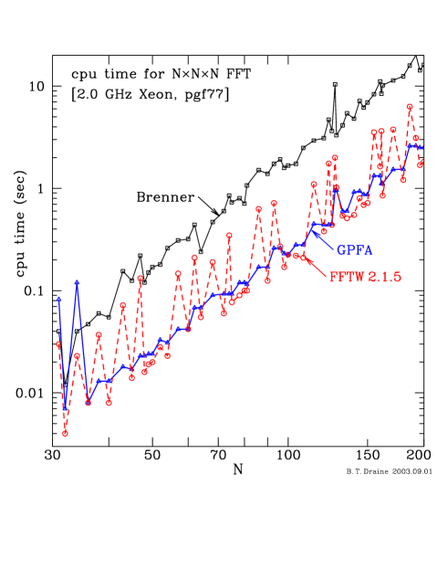
Figure 5: Comparison of cpu time required by 3 different FFT implementations. It is seen that the GPFA and FFTW implementations have comparable speeds, much faster than Brenner’s FFT implementation.

The GPFA routine is portable and quite fast: Figure 5 compares the speed of three FFT implementations: Brenner’s, GPFA, and FFTW (http://www.fftw.org). We see that while for some cases FFTW 2.1.5 is faster than the GPFA algorithm, the difference is only marginal. The FFTW code and GPFA code are quite comparable in performance – for some cases the GPFA code is faster, for other cases the FFTW code is faster. For target dimensions which are factorizable as $2^{i}3^{j}5^{k}$ (for integer $i$, $j$, $k$), the GPFA and FFTW codes have the same memory requirements. For targets with extents $N_{x}$, $N_{y}$, $N_{z}$ which are not factorizable as $2^{i}3^{j}5^{k}$, the GPFA code needs to “extend” the computational volume to have values of $N_{x}$, $N_{y}$, and $N_{z}$ which are factorizable by 2, 3, and 5. For these cases, GPFA requires somewhat more memory than FFTW. However, the fractional difference in required memory is not large, since integers factorizable as $2^{i}3^{j}5^{k}$ occur fairly frequently. [Note: This “extension” of the target volume occurs automatically and is transparent to the user.]

DDSCAT 7.3 offers a new FFT option: the Intel^® Math Kernel Library DFTI. This is tuned for optimum performance, and appears to offer real performance advantages on modern multi-core cpus. With this now available, the FFTW option, which had been included in DDSCAT 6.1, has been removed from DDSCAT 7.3.

The choice of FFT implementation is obtained by specifying one of:

• FFTMKL to use the Intel^® MKL routine DFTI (see §6.5). This is recommended, but requires that the Intel^® Math Kernel Library be installed on your system.

• GPFAFT to use the GPFA algorithm (Temperton 1992). This is not quite as fast as FFTMKL, but is written in plain Fortran-90. It is a perfectly good alternative if the Intel^® Math Kernel Library is not available on your system.

14 Choice of DDA Method

14.1 Point Dipoles: Options LATTDR and GKDLDR

Earlier versions of DDSCAT (up to and including DDSCAT 7.2 treated the well-defined problem of absorption and scattering by an array of polarizable points (Purcell & Pennypacker 1973; Draine 1988; Draine & Flatau 1994), where the target is divided up into finite elements, each represented by a polarizable point. The problem is then fully characterized by the geometric distribution of the polarizable points, the polarizability $\alpha$ of each point, and the incident electromagnetic wave. The polarizability $\alpha$ is chosen according to some prescription. Earlier versions of DDSCAT offered as options the “Lattice Dispersion Relation” prescription of Draine & Goodman (1993), and the modified Lattice Dispersion Relation prescription of Gutkowicz-Krusin & Draine (2004). Option GKDLDR specifies that the polarizability be prescribed by the “Lattice Dispersion Relation”, with the polarizability found by Gutkowicz-Krusin & Draine (2004), who corrected a subtle error in the analysis of Draine & Goodman (1993). For $|m|kd\lower 2.15277pt\hbox{$\;\buildrel<\over{\sim}\;$}1$, the GKDLDR polarizability differs slightly from the LATTDR polarizability, but the differences in calculated scattering cross sections are relatively small, as can be seen from Figure 6. We recommend option GKDLDR.

Users wishing to compare can invoke option LATTDR to specify that the “Lattice Dispersion Relation” of Draine & Goodman (1993) be employed to determine the dipole polarizabilities. This polarizability also works well.

This approach works well provided the refractive index $m$ of the target material is not too large. However, when $|m|$ is large, both of these methods perform poorly.

14.2 Filtered Coupled Dipole: option FLTRCD

Piller & Martin (1998) proposed the “filtered coupled dipole” (FCD) method as an approach that would work better for targets with large refractive indices. This method continues to represent a finite target by an array of polarizable points, but with the electric field generated by each point differing from the field of a true point dipole by virtue of having component of high spatial frequency “filtered out”. Gay-Balmaz & Martin (2002) revisited the FCD method, correcting some typographical errors in Piller & Martin (1998). Yurkin et al. (2010) carried out a comparison of the FCD method with the point dipole method and showed that the FCD method could be used for targets with large refractive indices where the the point dipole method failed.

DDSCAT 7.3 offers the filtered coupled dipole method as an option (FLTRDD). When this option is selected, the dipole polarizabilities are assigned by

$$\alpha_{j}=\frac{\alpha^{\rm(CM)}}{1+D}\leavevmode\nobreak\ \leavevmode\nobreak\ \leavevmode\nobreak\ ,$$ (20)

where $\alpha^{\rm(CM)}$ is the Clausius-Mossotti polarizability

$$\alpha^{\rm(CM)}\equiv\frac{3d^{3}}{4\pi}\frac{(m_{j}^{2}-1)}{(m_{j}^{2}+2)}\leavevmode\nobreak\ \leavevmode\nobreak\ \leavevmode\nobreak\ ,$$ (21)

where $m_{j}$ is the complex refractive index at lattice site $j$. The correction term $D$ is given by

$$D=\frac{\alpha^{\rm(CM)}}{d^{3}}\left[\frac{4}{3}(kd)^{2}+\frac{2}{3\pi}\ln\left[\frac{\pi-kd}{\pi+kd}\right]+\frac{2}{3}i(kd)^{3}\right]\leavevmode\nobreak\ \leavevmode\nobreak\ \leavevmode\nobreak\ ,$$ (22)

(see Yurkin et al. 2010, eq. 9). Here $d$ is the lattice spacing, and $k\equiv\omega/c$.

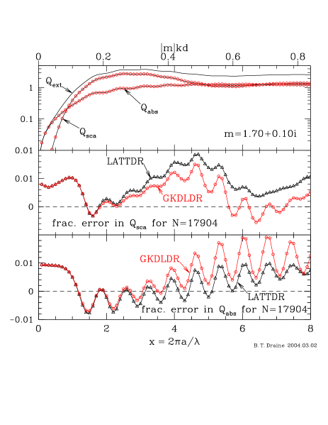
Figure 6: Scattering and absorption for a $m=1.7+0.1i$ sphere, calculated using two prescriptions for the polarizability: LATTDR is the lattice dispersion relation result of Draine & Goodman (1993). GKDLDR is the lattice dispersion relation result of Gutkowicz-Krusin & Draine (2004). Results are shown as a function of scattering parameter $x=2\pi a/\lambda$; the upper scale gives values of $|m|kd$. We see that the cross sections calculated with these two prescriptions are quite similar for $|m|kd\lower 1.72221pt\hbox{$\;\buildrel<\over{\sim}\;$}0.5$. For other examples see Gutkowicz-Krusin & Draine (2004).

15 Dielectric Functions

In order to assign the appropriate dipole polarizabilities, DDSCAT 7.3 must be given the refractive index $m$ or dielectric constant $\epsilon$ of the material (or materials) of which the target of interest is composed. This information is supplied to DDSCAT 7.3 through a table (or tables), read by subroutine DIELEC in file dielec.f90, and providing either the complex refractive index $m=n+ik$ or complex dielectric function $\epsilon=\epsilon_{1}+i\epsilon_{2}$ as a function of wavelength $\lambda$. Since $m=\epsilon^{1/2}$, or $\epsilon=m^{2}$, the user must supply either $m$ or $\epsilon$.

DDSCAT 7.3 can calculate scattering and absorption by targets with anisotropic dielectric functions, with arbitrary orientation of the optical axes relative to the target shape. See §28.

The table containing the dielectric function information should give $m$ or $\epsilon$ as a function of the wavelength in vacuo.

The table formatting is intended to be quite flexible. The first line of the table consists of text, up to 80 characters of which will be read and included in the output to identify the choice of dielectric function. (For the sample problem, it consists of simply the statement m = 1.33 + 0.01i.) The second line consists of 5 integers; either the second and third or the fourth and fifth should be zero.

• The first integer specifies which column the wavelength is stored in.

• The second integer specifies which column Re$(m)$ is stored in.

• The third integer specifies which column Im$(m)$ is stored in.

• The fourth integer specifies which column Re$(\epsilon)$ is stored in.

• The fifth integer specifies which column Im$(\epsilon)$ is stored in.

If the second and third integers are zeros, then DIELEC will read Re$(\epsilon)$ and Im$(\epsilon)$ from the file; if the fourth and fifth integers are zeros, then Re$(m)$ and Im$(m)$ will be read from the file.

The third line of the file is used for column headers, and the data begins in line 4. There must be at least 3 lines of data: even if $m$ or $\epsilon$ is required at only one wavelength, please supply two additional “dummy” wavelength entries in the table so that the interpolation apparatus will not be confused.

As discussed in §3.2, DDSCAT can scattering for targets embedded in dielectric media. The refractive index of the ambient medium is specified by the value of NAMBIENT in the parameter file ddscat.par (see §9.10).

Here is an example of a refractive index file for Au:

Gold, evaporated (Johnson & Christy 1972, PRB 6, 4370)
1 2 3 0 0 = columns for wave, Re(n), Im(n), eps1, eps2
wave(um) Re(n)  Im(n)   eps1   eps2
0.5486   0.43   2.455   -5.84  2.11
0.5209   0.62   2.081   -3.95  2.58
0.4959   1.04   1.833   -2.28  3.81
0.4714   1.31   1.849   -1.70  4.84
0.4509   1.38   1.914   -1.76  5.28
0.4305   1.45   1.948   -1.69  5.65
0.4133   1.46   1.958   -1.70  5.72
0.3974   1.47   1.952   -1.65  5.74
0.3815   1.46   1.933   -1.60  5.64
0.3679   1.48   1.895   -1.40  5.61
0.3542   1.50   1.866   -1.23  5.60
0.3425   1.48   1.871   -1.31  5.54
0.3315   1.48   1.883   -1.36  5.57
0.3204   1.54   1.898   -1.23  5.85
0.3107   1.53   1.893   -1.24  5.79
0.3009   1.53   1.889   -1.23  5.78

16 Calculation of $\langle\cos\theta\rangle$, Radiative Force, and Radiation Torque

In addition to solving the scattering problem for a dipole array, DDSCAT can compute the three-dimensional force ${\bf F}_{\rm rad}$ and torque ${\bf\Gamma}_{\rm rad}$ exerted on this array by the incident and scattered radiation fields. The radiation torque calculation is carried out, after solving the scattering problem, only if DOTORQ has been specified in ddscat.par. For each incident polarization mode, the results are given in terms of dimensionless efficiency vectors ${\bf Q}_{\rm pr}$ and ${\bf Q}_{\Gamma}$, defined by

$${\bf Q}_{\rm pr}\equiv{{\bf F}_{\rm rad}\over\pi{a}_{\rm eff}^{2}u_{\rm rad}}\leavevmode\nobreak\ \leavevmode\nobreak\ \leavevmode\nobreak\ ,$$ (23)

$${\bf Q}_{\Gamma}\equiv{k{\bf\Gamma}_{\rm rad}\over\pi{a}_{\rm eff}^{2}u_{\rm rad}}\leavevmode\nobreak\ \leavevmode\nobreak\ \leavevmode\nobreak\ ,$$ (24)

where ${\bf F}_{\rm rad}$ and ${\bf\Gamma}_{\rm rad}$ are the time-averaged force and torque on the dipole array, $k=2\pi/\lambda$ is the wavenumber in vacuo, and $u_{\rm rad}=E_{0}^{2}/8\pi$ is the time-averaged energy density for an incident plane wave with amplitude $E_{0}\cos(\omega t+\phi)$. The radiation pressure efficiency vector can be written

$${\bf Q}_{\rm pr}=Q_{\rm ext}{\hat{\bf k}}-Q_{\rm sca}{\bf g}\leavevmode\nobreak\ \leavevmode\nobreak\ \leavevmode\nobreak\ ,$$ (25)

where ${\hat{\bf k}}$ is the direction of propagation of the incident radiation, and the vector g is the mean direction of propagation of the scattered radiation:

$${\bf g}={1\over C_{\rm sca}}\int d\Omega{dC_{\rm sca}({\hat{\bf n}},{\hat{\bf k}})\over d\Omega}{\hat{\bf n}}\leavevmode\nobreak\ \leavevmode\nobreak\ \leavevmode\nobreak\ ,$$ (26)

where $d\Omega$ is the element of solid angle in scattering direction ${\hat{\bf n}}$, and $dC_{\rm sca}/d\Omega$ is the differential scattering cross section. The components of ${\bf Q}_{\rm pr}$ are reported in the Target Frame: $Q_{{\rm pr},1}\equiv{\bf F}_{\rm rad}\cdot\hat{\bf x}_{\rm TF}$, $Q_{{\rm pr},2}\equiv{\bf F}_{\rm rad}\cdot\hat{\bf y}_{\rm TF}$, $Q_{{\rm pr},3}\equiv{\bf F}_{\rm rad}\cdot\hat{\bf z}_{\rm TF}$.

Equations for the evaluation of the radiative force and torque are derived by Draine & Weingartner (1996). It is important to note that evaluation of ${\bf Q}_{\rm pr}$ and ${\bf Q}_{\Gamma}$ involves averaging over scattering directions to evaluate the linear and angular momentum transport by the scattered wave. This evaluation requires appropriate choices of the parameter ETASCA – see §25.

In addition, DDSCAT calculates $\langle\cos\theta\rangle$ [the first component of the vector $g$ in eq. (26)] and the second moment $\langle\cos^{2}\theta\rangle$. These two moments are useful measures of the anisotropy of the scattering. For example, Draine (2003) gives an analytic approximation to the scattering phase function of dust mixtures that is parameterized by the two moments $\langle\cos\theta\rangle$ and $\langle\cos^{2}\theta\rangle$.

17 Memory Requirements

The memory requirements are determined by the size of the “computational volume” – this is a rectangular region, of size NX$\times$NY$\times$NZ that is large enough to contain the target. If using the GPFAFT option, then NX, NY, NZ are also required to have only 2,3, and 5 as prime factors (see footnote 12).

In single precision, the memory requirement for DDSCAT 7.3 is approximately

$$(35.+0.0010\times{\tt NX}\times{\tt NY}\times{\tt NZ}){\rm\leavevmode\nobreak\ Mbytes}\leavevmode\nobreak\ \leavevmode\nobreak\ \leavevmode\nobreak\ \leavevmode\nobreak\ {\rm for\leavevmode\nobreak\ single\leavevmode\nobreak\ precision}$$ (27)

$$(42+0.0020\times{\tt NX}\times{\tt NY}\times{\tt NZ}){\rm\leavevmode\nobreak\ Mbytes}\leavevmode\nobreak\ \leavevmode\nobreak\ \leavevmode\nobreak\ \leavevmode\nobreak\ {\rm for\leavevmode\nobreak\ double\leavevmode\nobreak\ precision}$$ (28)

Thus, in single precision, a 48$\times$48$\times$48 calculation requires $\sim$146 MBytes.

The memory is allocated dynamically – once the target has been created, DDSCAT 7.3 will determine just how much overall memory is needed, and will allocate it. However, the user must provide information (via ddscat.par) to allow DDSCAT 7.3 to allocate sufficiently large arrays to carry out the initial target creation. Initially, the only arrays that will be allocated are those related to the target geometry, so it is OK to be quite generous in this initial allowance, as the memory required for the target generation step is small compared to the memory required to carry out the full scattering calculation.

18 Target Geometry: The Target Frame

The geometry of the target is specified by the locations of the lattice sites where polarizable points (“dipoles”) are located. The list of occupied sites will be generated internally by DDSCAT if the user selects one of the “built-in” target geometries, but the user can also use the target option FROM_FILE to read in the list of occupied site locations and composition information.

Every target is defined by a list of “occupied” lattice sites $(i,j,k)_{n}$, $n=1,...,N$. In the “Target Frame” (TF), these sites have physical locations $(x,y,z)_{n}=[(i,j,k)_{n}+(x_{0},y_{0},z_{0})]\times d$, where $d$ is the lattice constant (in physical units) and $(x_{0},y_{0},z_{0})$ is a vector that gives the physical location corresponding to $(i,j,k)=(0,0,0)$. Thus, the vector ${\bf x}_{0}$ specifies the physical location of the TF “lattice coordinate” origin $(0,0,0)_{\rm TF}$. The vector ${\bf x}_{0}$ is specified for for each of the “built-in” target geometries. For targets provided externally through the FROM_FILE option (see §21.1), the “target file” must include the three components of the vector ${\bf x}_{0}$.

19 Target Orientation

Recall that we define a “Lab Frame” (LF) in which the incident radiation propagates in the $+x$ direction. For purposes of discussion we will always let unit vectors $\hat{\bf x}_{\rm LF}$, $\hat{\bf y}_{\rm LF}$, $\hat{\bf z}_{\rm LF}=\hat{\bf x}_{\rm LF}\times\hat{\bf y}_{\rm LF}$ be the three coordinate axes of the LF.

In ddscat.par one specifies the first polarization state ${\hat{\bf e}}_{01}$ (which obviously must lie in the $y,z$ plane in the LF); DDSCAT automatically constructs a second polarization state ${\hat{\bf e}}_{02}=\hat{\bf x}_{\rm LF}\times{\hat{\bf e}}_{01}^{*}$ orthogonal to ${\hat{\bf e}}_{01}$. Users will often find it convenient to let polarization vectors ${\hat{\bf e}}_{01}={\hat{\bf y}}$, ${\hat{\bf e}}_{02}={\hat{\bf z}}$ (although this is not mandatory – see §24).

Figure 7: Target orientation in the Lab Frame. ${\hat{\bf x}}=\hat{\bf x}_{\rm LF}$ is the direction of propagation of the incident radiation, and ${\hat{\bf y}}=\hat{\bf y}_{\rm LF}$ is the direction of the real component (at $x_{\rm LF}=0$, $t=0$) of the first incident polarization mode. In this coordinate system, the orientation of target axis ${\hat{\bf a}}_{1}$ is specified by angles $\Theta$ and $\Phi$. With target axis ${\hat{\bf a}}_{1}$ fixed, the orientation of target axis ${\hat{\bf a}}_{2}$ is then determined by angle $\beta$ specifying rotation of the target around ${\hat{\bf a}}_{1}$. When $\beta=0$, ${\hat{\bf a}}_{2}$ lies in the ${\hat{\bf a}}_{1}$,$\hat{\bf x}_{\rm LF}$ plane.

Recall that definition of a target involves specifying two unit vectors, ${\hat{\bf a}}_{1}$ and ${\hat{\bf a}}_{2}$, which are imagined to be “frozen” into the target. We require ${\hat{\bf a}}_{2}$ to be orthogonal to ${\hat{\bf a}}_{1}$. Therefore we may define a “Target Frame" (TF) defined by the three unit vectors ${\hat{\bf a}}_{1}$, ${\hat{\bf a}}_{2}$, and ${\hat{\bf a}}_{3}={\hat{\bf a}}_{1}\times{\hat{\bf a}}_{2}$ .

For example, when DDSCAT creates a 32$\times$24$\times$16 rectangular solid, it fixes ${\hat{\bf a}}_{1}$ to be along the longest dimension of the solid, and ${\hat{\bf a}}_{2}$ to be along the next-longest dimension.

Important Note: for periodic targets, DDSCAT 7.3 requires that the periodic target have ${\hat{\bf a}}_{1}=\hat{\bf x}_{\rm TF}$ and ${\hat{\bf a}}_{2}=\hat{\bf y}_{\rm TF}$.

Orientation of the target relative to the incident radiation can in principle be determined two ways:

1. specifying the direction of ${\hat{\bf a}}_{1}$ and ${\hat{\bf a}}_{2}$ in the LF, or

2. specifying the directions of $\hat{\bf x}_{\rm LF}$ (incidence direction) and $\hat{\bf y}_{\rm LF}$ in the TF.

DDSCAT uses method 1.: the angles $\Theta$, $\Phi$, and $\beta$ are specified in the file ddscat.par. The target is oriented such that the polar angles $\Theta$ and $\Phi$ specify the direction of ${\hat{\bf a}}_{1}$ relative to the incident direction $\hat{\bf x}_{\rm LF}$, where the $\hat{\bf x}_{\rm LF}$,$\hat{\bf y}_{\rm LF}$ plane has $\Phi=0$. Once the direction of ${\hat{\bf a}}_{1}$ is specified, the angle $\beta$ then specifies how the target is to rotated around the axis ${\hat{\bf a}}_{1}$ to fully specify its orientation. A more extended and precise explanation follows:

19.1 Orientation of the Target in the Lab Frame

DDSCAT uses three angles, $\Theta$, $\Phi$, and $\beta$, to specify the directions of unit vectors ${\hat{\bf a}}_{1}$ and ${\hat{\bf a}}_{2}$ in the LF (see Fig. 7).

$\Theta$ is the angle between ${\hat{\bf a}}_{1}$ and $\hat{\bf x}_{\rm LF}$.

When $\Phi=0$, ${\hat{\bf a}}_{1}$ will lie in the $\hat{\bf x}_{\rm LF},\hat{\bf y}_{\rm LF}$ plane. When $\Phi$ is nonzero, it will refer to the rotation of ${\hat{\bf a}}_{1}$ around $\hat{\bf x}_{\rm LF}$: e.g., $\Phi=90^{\circ}$ puts ${\hat{\bf a}}_{1}$ in the $\hat{\bf x}_{\rm LF},\hat{\bf z}_{\rm LF}$ plane.

When $\beta=0$, ${\hat{\bf a}}_{2}$ will lie in the $\hat{\bf x}_{\rm LF},{\hat{\bf a}}_{1}$ plane, in such a way that when $\Theta=0$ and $\Phi=0$, ${\hat{\bf a}}_{2}$ is in the $\hat{\bf y}_{\rm LF}$ direction: e.g, $\Theta=90^{\circ}$, $\Phi=0$, $\beta=0$ has ${\hat{\bf a}}_{1}=\hat{\bf y}_{\rm LF}$ and ${\hat{\bf a}}_{2}=-\hat{\bf x}_{\rm LF}$. Nonzero $\beta$ introduces an additional rotation of ${\hat{\bf a}}_{2}$ around ${\hat{\bf a}}_{1}$: e.g., $\Theta=90^{\circ}$, $\Phi=0$, $\beta=90^{\circ}$ has ${\hat{\bf a}}_{1}=\hat{\bf y}_{\rm LF}$ and ${\hat{\bf a}}_{2}=\hat{\bf z}_{\rm LF}$.

Mathematically:

$${\hat{\bf a}}_{1} = \hat{\bf x}_{\rm LF}\cos\Theta+\hat{\bf y}_{\rm LF}\sin\Theta\cos\Phi+\hat{\bf z}_{\rm LF}\sin\Theta\sin\Phi$$ (29)

$${\hat{\bf a}}_{2} = -\hat{\bf x}_{\rm LF}\sin\Theta\cos\beta+\hat{\bf y}_{\rm LF}[\cos\Theta\cos\beta\cos\Phi-\sin\beta\sin\Phi]$$ (30)

$$+\hat{\bf z}_{\rm LF}[\cos\Theta\cos\beta\sin\Phi+\sin\beta\cos\Phi]$$

$${\hat{\bf a}}_{3} = \hat{\bf x}_{\rm LF}\sin\Theta\sin\beta-\hat{\bf y}_{\rm LF}[\cos\Theta\sin\beta\cos\Phi+\cos\beta\sin\Phi]$$ (31)

$$-\hat{\bf z}_{\rm LF}[\cos\Theta\sin\beta\sin\Phi-\cos\beta\cos\Phi]$$

or, equivalently:

$$\hat{\bf x}_{\rm LF} = {\hat{\bf a}}_{1}\cos\Theta-{\hat{\bf a}}_{2}\sin\Theta\cos\beta+{\hat{\bf a}}_{3}\sin\Theta\sin\beta$$ (32)

$$\hat{\bf y}_{\rm LF} = {\hat{\bf a}}_{1}\sin\Theta\cos\Phi+{\hat{\bf a}}_{2}[\cos\Theta\cos\beta\cos\Phi-\sin\beta\sin\Phi]$$ (33)

$$-{\hat{\bf a}}_{3}[\cos\Theta\sin\beta\cos\Phi+\cos\beta\sin\Phi]$$

$$\hat{\bf z}_{\rm LF} = {\hat{\bf a}}_{1}\sin\Theta\sin\Phi+{\hat{\bf a}}_{2}[\cos\Theta\cos\beta\sin\Phi+\sin\beta\cos\Phi]$$ (34)

$$-{\hat{\bf a}}_{3}[\cos\Theta\sin\beta\sin\Phi-\cos\beta\cos\Phi]$$

19.2 Orientation of the Incident Beam in the Target Frame

Under some circumstances, one may wish to specify the target orientation such that $\hat{\bf x}_{\rm LF}$ (the direction of propagation of the radiation) and $\hat{\bf y}_{\rm LF}$ (usually the first polarization direction) and $\hat{\bf z}_{\rm LF}$ (= $\hat{\bf x}_{\rm LF}\times\hat{\bf y}_{\rm LF}$) refer to certain directions in the TF. Given the definitions of the LF and TF above, this is simply an exercise in coordinate transformation. For example, one might wish to have the incident radiation propagating along the (1,1,1) direction in the TF (example 14 below). Here we provide some selected examples:

1. $\hat{\bf x}_{\rm LF}={\hat{\bf a}}_{1}$, $\hat{\bf y}_{\rm LF}={\hat{\bf a}}_{2}$, $\hat{\bf z}_{\rm LF}={\hat{\bf a}}_{3}$ : $\Theta=0$, $\Phi+\beta=0$

2. $\hat{\bf x}_{\rm LF}={\hat{\bf a}}_{1}$, $\hat{\bf y}_{\rm LF}={\hat{\bf a}}_{3}$, $\hat{\bf z}_{\rm LF}=-{\hat{\bf a}}_{2}$ : $\Theta=0$, $\Phi+\beta=-90^{\circ}$

3. $\hat{\bf x}_{\rm LF}={\hat{\bf a}}_{2}$, $\hat{\bf y}_{\rm LF}={\hat{\bf a}}_{1}$, $\hat{\bf z}_{\rm LF}=-{\hat{\bf a}}_{3}$ : $\Theta=90^{\circ}$, $\beta=180^{\circ}$, $\Phi=0$

4. $\hat{\bf x}_{\rm LF}={\hat{\bf a}}_{2}$, $\hat{\bf y}_{\rm LF}={\hat{\bf a}}_{3}$, $\hat{\bf z}_{\rm LF}={\hat{\bf a}}_{1}$ : $\Theta=90^{\circ}$, $\beta=180^{\circ}$, $\Phi=90^{\circ}$

5. $\hat{\bf x}_{\rm LF}={\hat{\bf a}}_{3}$, $\hat{\bf y}_{\rm LF}={\hat{\bf a}}_{1}$, $\hat{\bf z}_{\rm LF}={\hat{\bf a}}_{2}$ : $\Theta=90^{\circ}$, $\beta=90^{\circ}$, $\Phi=0$

6. $\hat{\bf x}_{\rm LF}={\hat{\bf a}}_{3}$, $\hat{\bf y}_{\rm LF}={\hat{\bf a}}_{2}$, $\hat{\bf z}_{\rm LF}=-{\hat{\bf a}}_{1}$ : $\Theta=90^{\circ}$, $\beta=90^{\circ}$, $\Phi=-90^{\circ}$

7. $\hat{\bf x}_{\rm LF}=-{\hat{\bf a}}_{1}$, $\hat{\bf y}_{\rm LF}={\hat{\bf a}}_{2}$, $\hat{\bf z}_{\rm LF}=-{\hat{\bf a}}_{3}$ : $\Theta=180^{\circ}$, $\beta-\Phi=180^{\circ}$

8. $\hat{\bf x}_{\rm LF}=-{\hat{\bf a}}_{1}$, $\hat{\bf y}_{\rm LF}={\hat{\bf a}}_{3}$, $\hat{\bf z}_{\rm LF}={\hat{\bf a}}_{2}$ : $\Theta=180^{\circ}$, $\beta-\Phi=90^{\circ}$

9. $\hat{\bf x}_{\rm LF}=-{\hat{\bf a}}_{2}$, $\hat{\bf y}_{\rm LF}={\hat{\bf a}}_{1}$, $\hat{\bf z}_{\rm LF}={\hat{\bf a}}_{3}$ : $\Theta=90^{\circ}$, $\beta=0$, $\Phi=0$

10. $\hat{\bf x}_{\rm LF}=-{\hat{\bf a}}_{2}$, $\hat{\bf y}_{\rm LF}={\hat{\bf a}}_{3}$, $\hat{\bf z}_{\rm LF}=-{\hat{\bf a}}_{1}$ : $\Theta=90^{\circ}$, $\beta=0$, $\Phi=-90^{\circ}$

11. $\hat{\bf x}_{\rm LF}=-{\hat{\bf a}}_{3}$, $\hat{\bf y}_{\rm LF}={\hat{\bf a}}_{1}$, $\hat{\bf z}_{\rm LF}=-{\hat{\bf a}}_{2}$ : $\Theta=90^{\circ}$, $\beta=-90^{\circ}$, $\Phi=0$

12. $\hat{\bf x}_{\rm LF}=-{\hat{\bf a}}_{3}$, $\hat{\bf y}_{\rm LF}={\hat{\bf a}}_{2}$, $\hat{\bf z}_{\rm LF}={\hat{\bf a}}_{1}$ : $\Theta=90^{\circ}$, $\beta=-90^{\circ}$, $\Phi=90^{\circ}$

13. $\hat{\bf x}_{\rm LF}=({\hat{\bf a}}_{1}+{\hat{\bf a}}_{2})/\surd 2$, $\hat{\bf y}_{\rm LF}={\hat{\bf a}}_{3}$, $\hat{\bf z}_{\rm LF}=({\hat{\bf a}}_{1}-{\hat{\bf a}}_{2})/\surd 2$ : $\Theta=45^{\circ}$, $\beta=180^{\circ}$, $\Phi=90^{\circ}$

14. $\hat{\bf x}_{\rm LF}=({\hat{\bf a}}_{1}+{\hat{\bf a}}_{2}+{\hat{\bf a}}_{3})/\surd 3$, $\hat{\bf y}_{\rm LF}=({\hat{\bf a}}_{1}-{\hat{\bf a}}_{2})/\surd 2$, $\hat{\bf z}_{\rm LF}=({\hat{\bf a}}_{1}+{\hat{\bf a}}_{2}-2{\hat{\bf a}}_{3})/\surd 6$ :
    $\Theta=54.7356^{\circ}$, $\beta=135^{\circ}$, $\Phi=30^{\circ}$.

19.3 Sampling in $\Theta$, $\Phi$, and $\beta$

The present version, DDSCAT 7.3, chooses the angles $\beta$, $\Theta$, and $\Phi$ to sample the intervals (BETAMI,BETAMX), (THETMI,THETMX), (PHIMIN,PHIMAX), where BETAMI, BETAMX, THETMI, THETMX, PHIMIN, PHIMAX are specified in ddscat.par . The prescription for choosing the angles is to:

• uniformly sample in $\beta$;

• uniformly sample in $\Phi$;

• uniformly sample in $\cos\Theta$.

This prescription is appropriate for random orientation of the target, within the specified limits of $\beta$, $\Phi$, and $\Theta$.

Note that when DDSCAT 7.3 chooses angles it handles $\beta$ and $\Phi$ differently from $\Theta$. The range for $\beta$ is divided into NBETA intervals, and the midpoint of each interval is taken. Thus, if you take BETAMI=0, BETAMX=90, NBETA=2 you will get $\beta=22.5^{\circ}$ and $67.5^{\circ}$. Similarly, if you take PHIMIN=0, PHIMAX=180, NPHI=2 you will get $\Phi=45^{\circ}$ and $135^{\circ}$.

Sampling in $\Theta$ is done quite differently from sampling in $\beta$ and $\Phi$. First, as already mentioned above, DDSCAT 7.3 samples uniformly in $\cos\Theta$, not $\Theta$. Secondly, the sampling depends on whether NTHETA is even or odd.

• If NTHETA is odd, then the values of $\Theta$ selected include the extreme values THETMI and THETMX; thus, THETMI=0, THETMX=90, NTHETA=3 will give you $\Theta=0,60^{\circ},90^{\circ}$.

• If NTHETA is even, then the range of $\cos\Theta$ will be divided into NTHETA intervals, and the midpoint of each interval will be taken; thus, THETMI=0, THETMX=90, NTHETA=2 will give you $\Theta=41.41^{\circ}$ and $75.52^{\circ}$ [$\cos\Theta=0.25$ and $0.75$].

The reason for this is that if odd NTHETA is specified, then the “integration” over $\cos\Theta$ is performed using Simpson’s rule for greater accuracy. If even NTHETA is specified, then the integration over $\cos\Theta$ is performed by simply taking the average of the results for the different $\Theta$ values.

If averaging over orientations is desired, it is recommended that the user specify an odd value of NTHETA so that Simpson’s rule will be employed.

20 Orientational Averaging

DDSCAT has been constructed to facilitate the computation of orientational averages. How to go about this depends on the distribution of orientations which is applicable.

20.1 Randomly-Oriented Targets

For randomly-oriented targets, we wish to compute the orientational average of a quantity $Q(\beta,\Theta,\Phi)$:

$$\langle Q\rangle={1\over 8\pi^{2}}\int_{0}^{2\pi}d\beta\int_{-1}^{1}d\cos\Theta\int_{0}^{2\pi}d\Phi\leavevmode\nobreak\ Q(\beta,\Theta,\Phi)\leavevmode\nobreak\ \leavevmode\nobreak\ \leavevmode\nobreak\ .$$ (35)

To compute such averages, all you need to do is edit the file ddscat.par so that DDSCAT knows what ranges of the angles $\beta$, $\Theta$, and $\Phi$ are of interest. For a randomly-oriented target with no symmetry, you would need to let $\beta$ run from 0 to $360^{\circ}$, $\Theta$ from 0 to $180^{\circ}$, and $\Phi$ from 0 to $360^{\circ}$.

For targets with symmetry, on the other hand, the ranges of $\beta$, $\Theta$, and $\Phi$ may be reduced. First of all, remember that averaging over $\Phi$ is relatively “inexpensive", so when in doubt average over 0 to $360^{\circ}$; most of the computational “cost" is associated with the number of different values of ($\beta$,$\Theta$) which are used. Consider a cube, for example, with axis ${\hat{\bf a}}_{1}$ normal to one of the cube faces; for this cube $\beta$ need run only from 0 to $90^{\circ}$, since the cube has fourfold symmetry for rotations around the axis ${\hat{\bf a}}_{1}$. Furthermore, the angle $\Theta$ need run only from 0 to $90^{\circ}$, since the orientation ($\beta$,$\Theta$,$\Phi$) is indistinguishable from ($\beta$, $180^{\circ}-\Theta$, $360^{\circ}-\Phi$).

For targets with symmetry, the user is encouraged to test the significance of $\beta$,$\Theta$,$\Phi$ on targets with small numbers of dipoles (say, of the order of 100 or so) but having the desired symmetry.

20.2 Nonrandomly-Oriented Targets

Some special cases (where the target orientation distribution is uniform for rotations around the $x$ axis = direction of propagation of the incident radiation), one may be able to use DDSCAT 7.3 with appropriate choices of input parameters. More generally, however, you will need to modify subroutine ORIENT to generate a list of NBETA values of $\beta$, NTHETA values of $\Theta$, and NPHI values of $\Phi$, plus two weighting arrays WGTA(1-NTHETA,1-NPHI) and WGTB(1-NBETA). Here WGTA gives the weights which should be attached to each ($\Theta$,$\Phi$) orientation, and WGTB gives the weight to be attached to each $\beta$ orientation. Thus each orientation of the target is to be weighted by the factor WGTA$\times$WGTB. For the case of random orientations, DDSCAT chooses $\Theta$ values which are uniformly spaced in $\cos\Theta$, and $\beta$ and $\Phi$ values which are uniformly spaced, and therefore uses uniform weights WGTB=1./NBETA

When NTHETA is even, DDSCAT sets WGTA=1./(NTHETA$\times$NPHI)

but when NTHETA is odd, DDSCAT uses Simpson’s rule when integrating over $\Theta$ and WGTA= (1/3 or 4/3 or 2/3)/(NTHETA$\times$NPHI)

Note that the program structure of DDSCAT may not be ideally suited for certain highly oriented cases. If, for example, the orientation is such that for a given $\Phi$ value only one $\Theta$ value is possible (this situation might describe ice needles oriented with the long axis perpendicular to the vertical in the Earth’s atmosphere, illuminated by the Sun at other than the zenith) then it is foolish to consider all the combinations of $\Theta$ and $\Phi$ which the present version of DDSCAT is set up to do. We hope to improve this in a future version of DDSCAT.

21 Target Generation: Isolated Finite Targets

DDSCAT contains routines to generate dipole arrays representing finite targets of various geometries, including spheres, ellipsoids, rectangular solids, cylinders, hexagonal prisms, tetrahedra, two touching ellipsoids, and three touching ellipsoids. The target type is specified by variable CSHAPE on line 9 of ddscat.par, up to 12 target shape parameters (SHPAR₁, SHPAR₂, SHPAR₃, …) on line 10. The target geometry is most conveniently described in a coordinate system attached to the target which we refer to as the “Target Frame” (TF), with orthonormal unit vectors $\hat{\bf x}_{\rm TF}$, $\hat{\bf y}_{\rm TF}$, $\hat{\bf z}_{\rm TF}\equiv\hat{\bf x}_{\rm TF}\times\hat{\bf y}_{\rm TF}$. Once the target is generated, the orientation of the target in the Lab Frame is accomplished as described in §19.

Every target generation routine will specify

• The “occupied” lattice sites;

• The composition associated with each occupied lattice site;

• Two “target axes” $\hat{\bf a}_{1}$ and $\hat{\bf a}_{2}$ that are used as references when specifying the target orientation; and

• The location of the Target Frame origin of coordinates.

Target geometries currently supported include:

• FROM_FILE : isotropic target material(s), geometry read from file (§21.1)

• ANIFRMFIL : anisotropic target material(s), geometry read from file (§21.2)

• ANIELLIPS : anisotropic ellipsoid (§21.3)

• ANI_ELL_2 : two touching anisotropic ellipsoids (single composition) (§21.4)

• ANI_ELL_3 : three touching anisotropic ellipsoids (single composition) (§21.5)

• ANIRCTNGL : anisotropic brick (§21.6)

• CONELLIPS : two concentric ellipsoids) (§21.7)

• CYLINDER1 : finite cylinder (§21.8)

• CYLNDRCAP : cylinder with hemispherical end-caps (§21.9)

• DSKRCTNGL : disk resting on a brick (§21.10)

• DW1996TAR : 13-block target used by Draine & Weingartner (1996) (§21.11)

• ELLIPSOID : ellipsoid (including spheroid and sphere) (§21.12)

• ELLIPSO_2 : two touching ellipsoids, different compositions allowed (§21.13)

• ELLIPSO_3 : three touching ellipsoids, different compositions allowed (§21.14)

• HEX_PRISM : finite hexagonal prism (§21.15)

• LAYRDSLAB : multilayer rectangular slab (§21.16)

• MLTBLOCKS : collection of cubic blocks (§21.17)

• RCTGLPRSM : rectangular prism (i.e., brick) (§21.18)

• RCTGLBLK3 : stack of 3 rectangular blocks (§21.19)

• SLAB_HOLE : rectangular slab with cylindrical hole (§21.20)

• SPHERES_N : collection of N spheres (§21.21)

• SPHROID_2 : two touching spheroids, different compositions allowed (§21.22)

• SPH_ANI_N : collection of N anisotropic spheres (§21.23)

• TETRAHDRN : tetrahedron (§21.24)

• TRNGLPRSM : triangular prism (§21.25)

• UNIAXICYL : finite cylinder of uniaxial material (§21.26)

Each is described below.

21.1 FROM_FILE = Target composed of possibly anisotropic material, defined by list of dipole locations and “compositions” obtained from a file

If anisotropic, the “microcrystals” in the target are assumed to be aligned with the principal axes of the dielectric tensor parallel to $\hat{\bf x}_{\rm TF}$, $\hat{\bf y}_{\rm TF}$, and $\hat{\bf z}_{\rm TF}$. This option causes DDSCAT to read the target geometry and composition information from a file shape.dat instead of automatically generating one of the geometries for which DDSCAT has built-in target generation capability. The shape.dat file is read by routine REASHP (file reashp.f90). The file shape.dat gives the number $N$ of dipoles in the target, the components of the “target axes” $\hat{\bf a}_{1}$ and $\hat{\bf a}_{2}$ in the Target Frame (TF), the vector $x_{0}(1-3)$ determining the correspondence between the integers IXYZ and actual coordinates in the TF, and specifications for the location and “composition” of each dipole. The user can customize REASHP as needed to conform to the manner in which the target description is stored in file shape.dat. However, as supplied, REASHP expects the file shape.dat to have the following structure:

• one line containing a description; the first 67 characters will be read and printed in various output statements

• N = number of dipoles in target

• $a_{1x}$ $a_{1y}$ $a_{1z}$ = x,y,z components (in TF) of $\bf{a}_{1}$

• $a_{2x}$ $a_{2y}$ $a_{2z}$ = x,y,z components (in TF) of $\bf{a}_{2}$

• $d_{x}/d$  $d_{y}/d$  $d_{z}/d$ = 1. 1. 1. = relative spacing of dipoles in $\hat{\bf x}_{\rm TF}$, $\hat{\bf y}_{\rm TF}$, $\hat{\bf z}_{\rm TF}$ directions

• $x_{0x}$  $x_{0y}$  $x_{0z}$ = TF coordinates $x_{\rm TF}/d$  $y_{\rm TF}/d$  $z_{\rm TF}/d$ corresponding to lattice site IXYZ= 0 0 0

• (line containing comments)

• $dummy$ IXYZ(1,1) IXYZ(1,2) IXYZ(1,3) ICOMP(1,1) ICOMP(1,2) ICOMP(1,3)

• $dummy$ IXYZ(2,1) IXYZ(2,2) IXYZ(2,3) ICOMP(2,1) ICOMP(2,2) ICOMP(2,3)

• $dummy$ IXYZ(3,1) IXYZ(3,2) IXYZ(3,3) ICOMP(3,1) ICOMP(3,2) ICOMP(3,3)

• …

• $dummy$ IXYZ(J,1) IXYZ(J,2) IXYZ(J,3) ICOMP(J,1) ICOMP(J,2) ICOMP(J,3)

• …

• $dummy$ IXYZ(N,1) IXYZ(N,2) IXYZ(N,3) ICOMP(N,1) ICOMP(N,2) ICOMP(N,3)

where $dummy$ is a number (integer or floating point)that might, for example, identify the dipole. This number will not be used in any calculations.
If the target material at location J is isotropic, ICOMP(J,1), ICOMP(J,2), and ICOMP(J,3) have the same value.

--- demo file for target option FROM_FILE (homogeneous,isotropic target) ---
8       = NAT
1.000   0.000   0.000   = target vector a1 (in TF)
0.000   1.000   0.000   = target vector a2 (in TF)
1.      1.      1.      = d_x/d  d_y/d  d_z/d  (normally 1 1 1)
0.5     0.5     0.5      = X0(1-3) = location in lattice of "target origin"
J    JX   JY   JZ  ICOMPX,ICOMPY,ICOMPZ
1     0    0    0   1  1  1
2     0    0    1   1  1  1
3     0    1    0   1  1  1
4     0    1    1   1  1  1
5     1    0    0   1  1  1
6     1    0    1   1  1  1
7     1    1    0   1  1  1
8     1    1    1   1  1  1

The above sample target consists of 8 dipoles arranged to represent a cube.
This example is homogeneous: All sites have composition 1
The target origin X0 is set to be at the center of the target
Note that ICOMPX,ICOMPY,ICOMPZ could differ, allowing treatment of anisotropic targets, provided the dielectric tensor at each location is diagonal in the TF.

--- demo file for target option FROM_FILE (inhomogeneous, isotropic target) ---
8       = NAT
1.000   0.000   0.000   = target vector a1 (in TF)
0.000   1.000   0.000   = target vector a2 (in TF)
1.      1.      1.      = d_x/d  d_y/d  d_z/d  (normally 1 1 1)
0.5     0.5     0.5      = X0(1-3) = location in lattice of "target origin"
J    JX   JY   JZ  ICOMPX,ICOMPY,ICOMPZ
1     0    0    0   1  1  1
2     0    0    1   1  1  1
3     0    1    0   1  1  1
4     0    1    1   1  1  1
5     1    0    0   2  2  2
6     1    0    1   2  2  2
7     1    1    0   2  2  2
8     1    1    1   2  2  2

This sample target consists of 8 dipoles arranged to represent a cube.
This example is inhomogeneous: The lower half of the cube (JX=0) has isotropic composition 1
The upper half of the cube (JX=1) has isotropic composition 2
The target origin X0 is set to be at the center of the target.
Note that ICOMPX, ICOMPY, ICOMPZ can be different, allowing treatment of anisotropic targets, provided the dielectric tensor at each location is diagonal in the TF.

21.1.1 Sample calculation in directory examples_exp/FROM_FILE

Subdirectory examples_exp/FROM_FILE contains ddscat.par for calculation of scattering by a $0.5{\mu{\rm m}}\times 1{\mu{\rm m}}\times 1{\mu{\rm m}}$ Au block, represented by a $32\times 64\times 64=131072$ dipole array, as well as the output files from the calculation. The target geometry is input via the file shape.dat.

This target has $V=0.5{\mu{\rm m}}^{3}$, and ${a}_{\rm eff}=(3V/4\pi)^{1/3}=0.49237{\mu{\rm m}}$. The calculation is for an incident wavelength $\lambda=0.50{\mu{\rm m}}$; the Au has refractive index $m=0.9656+1.8628i$. The CCG method used is PBCGS2; the two orthogonal polarization require 29 and 30 iterations, respectively, to converge to the specified tolerance TOL = 1e-5. The computation used 165 MB of RAM, and required 208 cpu sec on a 2.53 GHz cpu.

N.B.: This is the same physical problem as the example in examples_exp/RCTGLPRSM (see §21.18.1), differing only in that in the present calculation the target geometry is input through the file shape.dat rather than generated by ddscat.

21.2 ANIFRMFIL = General anistropic target defined by list of dipole locations,“compositions”, and material orientations obtained from a file

This option causes DDSCAT to read the target geometry information from a file shape.dat instead of automatically generating one of the geometries listed below. The file shape.dat gives the number $N$ of dipoles in the target, the components of the “target axes” $\hat{\bf a}_{1}$ and $\hat{\bf a}_{2}$ in the Target Frame (TF), the vector $x_{0}(1-3)$ determining the correspondence between the integers IXYZ and actual coordinates in the TF, and specifications for the location and “composition” of each dipole. For each dipole $J$, the file shape.dat provides the location IXYZ($J$,1-3), the composition identifier integer ICOMP($J$,1-3) specifying the dielectric function corresponding to the three principal axes of the dielectric tensor, and angles $\Theta_{\rm DF}$, $\Phi_{\rm DF}$, and $\beta_{\rm DF}$ specifying the orientation of the local “Dielectric Frame” (DF) relative to the “Target Frame” (TF) (see §28). The DF is the reference frame in which the dielectric tensor is diagonalized. The Target Frame is the reference frame in which we specify the dipole locations.

The shape.dat file is read by routine REASHP (file reashp.f90). The user can customize REASHP as needed to conform to the manner in which the target geometry is stored in file shape.dat. However, as supplied, REASHP expects the file shape.dat to have the following structure:

• one line containing a description; the first 67 characters will be read and printed in various output statements.

• N = number of dipoles in target

• $a_{1x}$ $a_{1y}$ $a_{1z}$ = x,y,z components (in Target Frame) of $\bf{a}_{1}$

• $a_{2x}$ $a_{2y}$ $a_{2z}$ = x,y,z components (in Target Frame) of $\bf{a}_{2}$

• $d_{x}/d$  $d_{y}/d$  $d_{z}/d$ = 1. 1. 1. = relative spacing of dipoles in $\hat{\bf x}_{\rm TF}$, $\hat{\bf y}_{\rm TF}$, $\hat{\bf z}_{\rm TF}$ directions

• $x_{0x}$  $x_{0y}$  $x_{0z}$ = TF coordinates $x_{\rm TF}/d$  $y_{\rm TF}/d$  $z_{\rm TF}/d$ corresponding to lattice site IXYZ= 0 0 0

• (line containing comments)

• $dummy$ IXYZ(1,1-3) ICOMP(1,1-3) THETADF(1) PHIDF(1) BETADF(1)

• $dummy$ IXYZ(2,1-3) ICOMP(2,1-3) THETADF(2) PHIDF(2) BETADF(2)

• $dummy$ IXYZ(3,1-3) ICOMP(3,1-3) THETADF(3) PHIDF(3) BETADF(3)

• …

• $dummy$ IXYZ(J,1-3) ICOMP(J,1-3) THETADF(J) PHIDF(J) BETADF(J)

• …

• $dummy$ IXYZ(N,1-3) ICOMP(N,1-3) THETADF(N) PHIDF(N) BETADF(N)

Where $dummy$ is a number (either integer or floating point) that might, for example, give the number identifying the dipole. This number will not be used in any calculations.
THETADF PHIDF BETADF should be given in radians.

Here is an example of the first few lines of a target description file suitable for target option ANIFRMFIL:

--- demo file for target option ANIFRMFIL (this line is for comments) ---
8       = NAT
1.000   0.000   0.000   = target vector a1 (in TF)
0.000   1.000   0.000   = target vector a2 (in TF)
1.      1.      1.      = d_x/d  d_y/d  d_z/d  (normally 1 1 1)
0.      0.      0.      = X0(1-3) = location in lattice of "target origin"
J    JX   JY   JZ  ICOMP(J,1-3) THETADF PHIDF BETADF
1     0    0    0   1  1  1    0.     0.      0.
2     0    0    1   1  1  1    0.     0.      0.
3     0    1    0   1  1  1    0.     0.      0.
4     0    1    1   1  1  1    0.     0.      0.
5     1    0    0   2  3  3    0.5236 1.5708  0.
6     1    0    1   2  3  3    0.5236 1.5708  0.
7     1    1    0   2  3  3    0.5236 1.5708  0.
8     1    1    1   2  3  3    0.5236 1.5708  0.

This sample target consists of 8 dipoles arranged to represent a cube.
Half of the cube (dipoles with JX=0) has isotropic composition 1. For this case, the angles THETADF, PHIDF, BETADF do not matter, and it convenient to set them all to zero.
The other half of the cube (dipoles with JX=1) consists of a uniaxial material, with dielectric function 2 for E fields parallel to one axis (the “c-axis”), and dielectric function 3 for E fields perpendicular to the c-axis. The c-axis is $30^{o}$ (0.5236 radians) away from $\hat{\bf x}_{\rm TF}$, and lies in the $\hat{\bf x}_{\rm TF}$-$\hat{\bf z}_{\rm TF}$ plane (having been rotated by 1.5708 radians around $\hat{\bf x}_{\rm TF}$).
Note that ICOMP(J,K) can be different for K=1,3, allowing treatment of anisotropic targets, provided the dielectric tensor at each location is diagonal in the TF.

21.3 ANIELLIPS = Homogeneous, anisotropic ellipsoid.

SHPAR₁, SHPAR₂, SHPAR₃ define the ellipsoidal boundary:

$$\left(\frac{x_{\rm TF}/d}{{\tt SHPAR}_{1}}\right)^{2}+\left(\frac{y_{\rm TF}/d}{{\tt SHPAR}_{2}}\right)^{2}+\left(\frac{z_{\rm TF}/d}{{\tt SHPAR}_{3}}\right)^{2}=\frac{1}{4}\leavevmode\nobreak\ \leavevmode\nobreak\ \leavevmode\nobreak\ ,$$ (36)

The TF origin is located at the centroid of the ellipsoid.

21.4 ANI_ELL_2 = Two touching, homogeneous, anisotropic ellipsoids, with distinct compositions

Geometry as for ELLIPSO_2; SHPAR₁, SHPAR₂, SHPAR₃ have same meanings as for ELLIPSO_2. Target axes ${\hat{\bf a}}_{1}=(1,0,0)_{\rm TF}$ and ${\hat{\bf a}}_{2}=(0,1,0)_{\rm TF}$.
Line connecting ellipsoid centers is $\parallel\hat{\bf a}_{1}=\hat{\bf x}_{\rm TF}$.
TF origin is located between ellipsoids, at point of contact.
It is assumed that (for both ellipsoids) the dielectric tensor is diagonal in the TF. User must set NCOMP=6 and provide $xx$, $yy$, $zz$ components of dielectric tensor for first ellipsoid, and $xx$, $yy$, $zz$ components of dielectric tensor for second ellipsoid (ellipsoids are in order of increasing $x_{\rm TF}$).

21.5 ANI_ELL_3 = Three touching homogeneous, anisotropic ellipsoids with same size and orientation but distinct dielectric tensors

SHPAR₁, SHPAR₂, SHPAR₃ have same meanings as for ELLIPSO_3.
Target axis ${\hat{\bf a}}_{1}=(1,0,0)_{\rm TF}$ (along line of ellipsoid centers), and ${\hat{\bf a}}_{2}=(0,1,0)_{\rm TF}$.
TF origin is located at center of middle ellipsoid.
It is assumed that dielectric tensors are all diagonal in the TF. User must set NCOMP=9 and provide $xx$, $yy$, $zz$ elements of dielectric tensor for first ellipsoid, $xx$, $yy$, $zz$ elements for second ellipsoid, and $xx$, $yy$, $zz$ elements for third ellipsoid (ellipsoids are in order of increasing $x_{\rm TF}$).

21.6 ANIRCTNGL = Homogeneous, anisotropic, rectangular solid

x, y, z lengths/$d$ = SHPAR₁, SHPAR₂, SHPAR₃.
Target axes ${\hat{\bf a}}_{1}=(1,0,0)_{\rm TF}$ and ${\hat{\bf a}}_{2}=(0,1,0)_{\rm TF}$ in the TF.
$(x_{\rm TF},y_{\rm TF},z_{\rm TF})=(0,0,0)$ at middle of upper target surface, (where “up” = $\hat{\bf x}_{\rm TF}$). (The target surface is taken to be $d/2$ about the upper dipole layer.)
Dielectric tensor is assumed to be diagonal in the target frame.
User must set NCOMP=3 and supply names of three files for $\epsilon$ as a function of wavelength or energy: first for $\epsilon_{xx}$, second for $\epsilon_{yy}$, and third for $\epsilon_{zz}$,

21.6.1 Sample calculation in directory examples_exp/ANIRCTNGL

Subdirectory examples_exp/ANIRCTNGL contains ddscat.par for calculation of scattering by a $0.1{\mu{\rm m}}\times 0.2{\mu{\rm m}}\times 0.2{\mu{\rm m}}$ rectangular brick (${a}_{\rm eff}=0.098475{\mu{\rm m}}$) with an anisotropic dielectric tensor: $m=1.33+0.01i$ for ${\bf E}\parallel\hat{\bf x}_{\rm TF}$ and ${\bf E}\parallel\hat{\bf y}_{\rm TF}$, and $m=1.50+0.01i$ for ${\bf E}\parallel\hat{\bf z}_{\rm TF}$. Radiation is incident with ${\bf k}_{0}\parallel\hat{\bf x}_{\rm TF}$, with $\lambda=0.5{\mu{\rm m}}$. The ddscat.par file is as follows:

’ ============ Parameter file for v7.3 ===================’
’**** Preliminaries ****’
’NOTORQ’ = CMDTRQ*6 (DOTORQ, NOTORQ) -- either do or skip torque calculations
’PBCGS2’ = CMDSOL*6 (PBCGS2, PBCGST, PETRKP) -- CCG method
’GPFAFT’ = CMETHD*6 (GPFAFT, FFTMKL) -- FFT method
’GKDLDR’ = CALPHA*6 (GKDLDR, LATTDR, FLTRCD) -- DDA method
’NOTBIN’ = CBINFLAG (ALLBIN, ORIBIN, NOTBIN)
’**** Initial Memory Allocation ****’
10 20 20 = upper bound on target extent
’**** Target Geometry and Composition ****’
’ANIRCTNGL’ = CSHAPE*9 shape directive
10 20 20 = shape parameters SHPAR1, SHPAR2, SHPAR3
3         = NCOMP = number of dielectric materials
’../diel/m1.33_0.01’ = name of file containing dielectric function
’../diel/m1.33_0.01’
’../diel/m1.50_0.01’
’**** Additional Nearfield calculation? ****’
0 = NRFLD (=0 to skip nearfield calc., =1 to calculate nearfield E)
0.0 0.0 0.0 0.0 0.0 0.0 (fract. extens. of calc. vol. in -x,+x,-y,+y,-z,+z)
’**** Error Tolerance ****’
1.00e-5 = TOL = MAX ALLOWED (NORM OF |G>=AC|E>-ACA|X>)/(NORM OF AC|E>)
’**** maximum number of iterations allowed ****’
300     = MXITER
’**** Interaction cutoff parameter for PBC calculations ****’
5.00e-3 = GAMMA (1e-2 is normal, 3e-3 for greater accuracy)
’**** Angular resolution for calculation of <cos>, etc. ****’
2.0     = ETASCA (number of angles is proportional to [(2+x)/ETASCA]^2 )
’**** Vacuum wavelengths (micron) ****’
0.5 0.5 1 ’LIN’ = wavelengths (first,last,how many,how=LIN,INV,LOG)
’**** Refractive index of ambient medium’
1.000 = NAMBIENT
’**** Effective Radii (micron) **** ’
0.098475 0.098457 1 ’LIN’ = eff. radii (first, last, how many, how=LIN,INV,LOG)
’**** Define Incident Polarizations ****’
(0,0) (1.,0.) (0.,0.) = Polarization state e01 (k along x axis)
2 = IORTH  (=1 to do only pol. state e01; =2 to also do orth. pol. state)
’**** Specify which output files to write ****’
1 = IWRKSC (=0 to suppress, =1 to write ".sca" file for each target orient.
’**** Prescribe Target Rotations ****’
 0.   0.  1  = BETAMI, BETAMX, NBETA (beta=rotation around a1)
 0.   0.  1  = THETMI, THETMX, NTHETA (theta=angle between a1 and k)
 0.   0.  1  = PHIMIN, PHIMAX, NPHI (phi=rotation angle of a1 around k)
’**** Specify first IWAV, IRAD, IORI (normally 0 0 0) ****’
0   0   0    = first IWAV, first IRAD, first IORI (0 0 0 to begin fresh)
’**** Select Elements of S_ij Matrix to Print ****’
6       = NSMELTS = number of elements of S_ij to print (not more than 9)
11 12 21 22 31 41       = indices ij of elements to print
’**** Specify Scattered Directions ****’
’LFRAME’ = CMDFRM*6 (’LFRAME’ or ’TFRAME’ for Lab Frame or Target Frame)
2 = number of scattering planes
0.  0. 180. 30 = phi, thetan_min, thetan_max, dtheta (in degrees) for plane A
90. 0. 180. 30 = phi, ... for plane B

This calculation required 0.22 cpu sec on a 2.53 GHz cpu.

21.7 CONELLIPS = Two concentric ellipsoids

SHPAR₁, SHPAR₂, SHPAR₃ = lengths/$d$ of the outer ellipsoid along the $\hat{\bf x}_{\rm TF}$, $\hat{\bf y}_{\rm TF}$, $\hat{\bf z}_{\rm TF}$ axes;
SHPAR₄, SHPAR₅, SHPAR₆ = lengths/$d$ of the inner ellipsoid along the $\hat{\bf x}_{\rm TF}$, $\hat{\bf y}_{\rm TF}$, $\hat{\bf z}_{\rm TF}$ axes.
Target axes ${\hat{\bf a}}_{1}=(1,0,0)_{\rm TF}$, ${\hat{\bf a}}_{2}=(0,1,0)_{\rm TF}$.
TF origin is located at centroids of ellipsoids.
The “core" within the inner ellipsoid is composed of isotropic material 1; the “mantle" between inner and outer ellipsoids is composed of isotropic material 2.
User must set NCOMP=2 and provide dielectric functions for “core” and “mantle” materials.

21.8 CYLINDER1 = Homogeneous, isotropic finite cylinder

SHPAR₁ = length/$d$, SHPAR₂ = diameter/$d$, with
SHPAR₃ = 1 for cylinder axis $\hat{\bf a}_{1}\parallel\hat{\bf x}_{\rm TF}$: $\hat{\bf a}_{1}=(1,0,0)_{\rm TF}$ and $\hat{\bf a}_{2}=(0,1,0)_{\rm TF}$;
SHPAR₃ = 2 for cylinder axis $\hat{\bf a}_{1}\parallel\hat{\bf y}_{\rm TF}$: $\hat{\bf a}_{1}=(0,1,0)_{\rm TF}$ and $\hat{\bf a}_{2}=(0,0,1)_{\rm TF}$;
SHPAR₃ = 3 for cylinder axis $\hat{\bf a}_{1}\parallel\hat{\bf z}_{\rm TF}$: $\hat{\bf a}_{1}=(0,0,1)_{\rm TF}$ and $\hat{\bf a}_{2}=(1,0,0)_{\rm TF}$ in the TF.
TF origin is located at centroid of cylinder.
User must set NCOMP=1.

21.9 CYLNDRCAP = Homogeneous, isotropic finite cylinder with hemispherical endcaps.

SHPAR₁ = cylinder length/$d$ (not including end-caps!) and SHPAR₂ = cylinder diameter/$d$, with cylinder axis $={\hat{\bf a}}_{1}=(1,0,0)_{\rm TF}$ and ${\hat{\bf a}}_{2}=(0,1,0)_{\rm TF}$. The total length along the target axis (including the endcaps) is (SHPAR₁+SHPAR₂)$d$.
TF origin is located at centroid of cylinder.
User must set NCOMP=1.

21.10 DSKRCTNGL = Disk on top of a homogeneous rectangular slab

This option causes DDSCAT to create a target consisting of a disk of composition 1 resting on top of a rectangular block of composition 2. Materials 1 and 2 are assumed to be homogeneous and isotropic.
ddscat.par should set NCOMP to 2 .  
The cylindrical disk has thickness SHPAR₁$\times d$ in the x-direction, and diameter SHPAR₂$\times d$. The rectangular block is assumed to have thickness SHPAR₃$\times$d in the x-direction, length SHPAR₄$\times d$ in the y-direction, and length SHPAR₅$\times d$ in the z-direction. The lower surface of the cylindrical disk is in the $x=0$ plane. The upper surface of the slab is also in the $x=0$ plane.

The Target Frame origin (0,0,0) is located where the symmetry axis of the disk intersects the $x=0$ plane (the upper surface of the slab, and the lower surface of the disk). In the Target Frame, dipoles representing the rectangular block are located at $(x/d,y/d,z/d)=(j_{x}+0.5,j_{y}+\Delta_{y},j_{z}+\Delta_{z})$, where $j_{x}$, $j_{y}$, and $j_{z}$ are integers. $\Delta_{y}=0$ or 0.5 depending on whether SHPAR₄ is even or odd. $\Delta_{z}=0$ or 0.5 depending on whether SHPAR₅ is even or odd.

Dipoles representing the disk are located at
         $x/d=0.5,1.5,...,[{\rm int}({\tt SHPAR}_{4}+0.5)-0.5]$

As always, the physical size of the target is fixed by specifying the value of the effective radius ${a}_{\rm eff}\equiv(3V_{\rm T}/4\pi)^{1/3}$, where $V_{\rm T}$ is the total volume of solid material in the target. For this geometry, the number of dipoles in the target will be approximately $N=[{\tt SHPAR}_{1}\times{\tt SHPAR}_{2}\times{\tt SHPAR}_{3}+(\pi/4)(({\tt SHPAR}_{4})^{2}\times{\tt SHPAR}_{5})]$, although the exact number may differ because of the dipoles are required to be located on a rectangular lattice. The dipole spacing $d$ in physical units is determined from the specified value of ${a}_{\rm eff}$ and the number $N$ of dipoles in the target: $d=(4\pi/3N)^{1/3}{a}_{\rm eff}$. This option requires 5 shape parameters:
The pertinent line in ddscat.par should read
 
SHPAR₁ SHPAR₂ SHPAR₃ SHPAR₄ SHPAR₅
 
where
SHPAR₁ = [disk thickness (in $\hat{\bf x}_{\rm TF}$ direction)]/$d$ [material 1]
SHPAR₂ = (disk diameter)/$d$
SHPAR₃ = (brick thickness in $\hat{\bf x}_{\rm TF}$ direction)/$d$ [material 2]
SHPAR₄ = (brick thickness in $\hat{\bf y}_{\rm TF}$ direction)/$d$
SHPAR₅ = (brick thickness in $\hat{\bf z}_{\rm TF}$ direction)/$d$
 
The overall size of the target (in terms of numbers of dipoles) is determined by parameters (SHPAR1+SHPAR4), SHPAR₂, and SHPAR₃. The periodicity in the TF $y$ and $z$ directions is determined by parameters SHPAR₄ and SHPAR₅.
The physical size of the TUC is specified by the value of ${a}_{\rm eff}$ (in physical units, e.g. cm), specified in the file ddscat.par.

The “computational volume” is determined by (SHPAR₁+SHPAR₄)$\times$SHPAR₂$\times$SHPAR₃.

The target axes (in the TF) are set to ${\hat{\bf a}}_{1}=\hat{\bf x}_{\rm TF}=(1,0,0)_{\rm TF}$ – i.e., normal to the “slab” – and ${\hat{\bf a}}_{2}=\hat{\bf y}_{\rm TF}=(0,1,0)_{\rm TF}$. The orientation of the incident radiation relative to the target is, as for all other targets, set by the usual orientation angles $\Theta$, $\Phi$, and $\beta$ (see §19 above); for example, $\Theta=0$ would be for radiation incident normal to the slab.

21.11 DW1996TAR = 13 block target used by Draine & Weingartner (1996).

Single, isotropic material. Target geometry was used in study by Draine & Weingartner (1996) of radiative torques on irregular grains. ${\hat{\bf a}}_{1}$ and ${\hat{\bf a}}_{2}$ are principal axes with largest and second-largest moments of inertia. User must set NCOMP=1. Target size is controlled by shape parameter SHPAR(1) = width of one block in lattice units.
TF origin is located at centroid of target.

21.12 ELLIPSOID = Homogeneous, isotropic ellipsoid.

“Lengths” SHPAR₁, SHPAR₂, SHPAR₃ in the $x$, $y$, $z$ directions in the TF:

$$\left(\frac{x_{\rm TF}}{{\tt SHPAR}_{1}d}\right)^{2}+\left(\frac{y_{\rm TF}}{{\tt SHPAR}_{2}d}\right)^{2}+\left(\frac{z_{\rm TF}}{{\tt SHPAR}_{3}d}\right)^{2}=\frac{1}{4}\leavevmode\nobreak\ \leavevmode\nobreak\ \leavevmode\nobreak\ ,$$ (37)

where $d$ is the interdipole spacing.
The target axes are set to ${\hat{\bf a}}_{1}=(1,0,0)_{\rm TF}$ and ${\hat{\bf a}}_{2}=(0,1,0)_{\rm TF}$.
Target Frame origin = centroid of ellipsoid.
User must set NCOMP=1 on line 9 of ddscat.par.
A homogeneous, isotropic sphere is obtained by setting SHPAR₁ = SHPAR₂ = SHPAR₃ = diameter/$d$.

21.12.1 Sample calculation in directory examples_exp/ELLIPSOID

The directory examples_exp/ELLIPSOID contains ddscat.par for calculation of scattering by a sphere with refractive index $m=1.5+0.01i$ and $2\pi a/\lambda=5$, represented by a $N=59728$ dipole pseudosphere just fitting within a $48\times 48\times 48$ computational volume, as well as the output files from the calculation. The calculation with $2\pi a/\lambda=5$ has $|m|kd=0.309$. The computation used 144 MB of RAM and required 63 cpu sec on a 2.53 GHz cpu.

21.12.2 Sample calculation in directory examples_exp/ELLIPSOID_NEARFIELD

The directory examples_exp/ELLIPSOID_NEARFIELD contains ddscat.par for calculation of (1) far-field scattering and (2) ${\bf E}$ in and near the target for a sphere with refractive index $m=0.96+1.01i$ (refractive index of Au at $\lambda=0.5{\mu{\rm m}}$) and $2\pi a/\lambda=5$. The spherical target is represented by a $N=59728$ dipole pseudosphere just fitting within a $48\times 48\times 48$ computational volume, as well as the output files from the calculation.

In physical units with $\lambda=0.5{\mu{\rm m}}$, ${a}_{\rm eff}=5\times\lambda/2\pi=0.39789{\mu{\rm m}}$. The calculation with $2\pi a/\lambda=5$ has $|m|kd=0.309$. The computation used 144 MB of RAM and required 60 cpu sec on a 2.53 GHz cpu.

The nearfield calculation is specified to extend throughout a computational volume extending the original $48d\times 48d\times 48d$ computational volume by 50% in all directions, to become a $96d\times 96d\times 96d$ volume centered on the sphere. ${\bf E}$ is evaluated at all points in this volume. The nearfield calculation used 62 MB of RAM and required just 9.6 cpu sec. The nearfield calculation creates the binary files w000r000k000.E1 and w000r000k000.E2, one for each of the two incident polarizations.

After the nearfield calculation is complete, the program ddpostprocess is used to read the file w000r000k000.E1 (specified in ddpostprocess.par) and extract ${\bf E}$ at 501 points along a line specified in ddpostprocess.par – the line runs along the $\hat{\bf x}_{\rm TF}$ axis through the center of the sphere. The results are shown in Figure 8.

Figure 8: Normalized electric field intensity $|{\bf E}|^{2}/|{\bf E}_{0}|^{2}$ along a line parallel to the direction of propagation, and passing through the center of an Au sphere of radius $a=0.3979{\mu{\rm m}}$, for light with wavelength $\lambda=0.5{\mu{\rm m}}$. The calculation in examples_exp/ELLIPSOID_NEARFIELD was done with dipole spacing $d=a/48.49=0.00821{\mu{\rm m}}$.

21.13 ELLIPSO_2 = Two touching, homogeneous, isotropic ellipsoids, with distinct compositions

SHPAR₁, SHPAR₂, SHPAR₃=x-length/$d$, y-length/$d$, $z$-length/$d$ of one ellipsoid. The two ellipsoids have identical shape, size, and orientation, but distinct dielectric functions. The line connecting ellipsoid centers is along the $\hat{\bf x}_{\rm TF}$-axis. Target axes ${\hat{\bf a}}_{1}=(1,0,0)_{\rm TF}$ [along line connecting ellipsoids] and ${\hat{\bf a}}_{2}=(0,1,0)_{\rm TF}$.
Target Frame origin = midpoint between ellipsoids (where ellipsoids touch).
User must set NCOMP=2 and provide dielectric function file names for both ellipsoids. Ellipsoids are in order of increasing $x_{\rm TF}$: first dielectric function is for ellipsoid with center at negative $x_{\rm TF}$, second dielectric function for ellipsoid with center at positive $x_{\rm TF}$.

21.14 ELLIPSO_3 = Three touching homogeneous, isotropic ellipsoids of equal size and orientation, but distinct compositions

SHPAR₁, SHPAR₂, SHPAR₃ have same meaning as for ELLIPSO_2. Line connecting ellipsoid centers is parallel to $\hat{\bf x}_{\rm TF}$ axis. Target axis ${\hat{\bf a}}_{1}=(1,0,0)_{\rm TF}$ (along line of ellipsoid centers), and ${\hat{\bf a}}_{2}=(0,1,0)_{\rm TF}$.
Target Frame origin = centroid of middle ellipsoid.
User must set NCOMP=3 and provide (isotropic) dielectric functions for first, second, and third ellipsoid.

21.15 HEX_PRISM = Homogeneous, isotropic hexagonal prism

SHPAR₁ = (Length of prism)/$d$ = (distance between hexagonal faces)/$d$,
SHPAR₂ = (distance between opposite vertices of one hexagonal face)/$d$ = 2$\times$hexagon side/$d$.
SHPAR₃ selects one of 6 orientations of the prism in the Target Frame (TF).
Target axis ${\hat{\bf a}}_{1}$ is along the prism axis (i.e., normal to the hexagonal faces), and target axis ${\hat{\bf a}}_{2}$ is normal to one of the rectangular faces. There are 6 options for SHPAR₃:
SHPAR₃ = 1 for ${\hat{\bf a}}_{1}\parallel\hat{\bf x}_{\rm TF}$ and ${\hat{\bf a}}_{2}\parallel\hat{\bf y}_{\rm TF}$ ; SHPAR₃ = 2 for ${\hat{\bf a}}_{1}\parallel\hat{\bf x}_{\rm TF}$ and ${\hat{\bf a}}_{2}\parallel\hat{\bf z}_{\rm TF}$ ;
SHPAR₃ = 3 for ${\hat{\bf a}}_{1}\parallel\hat{\bf y}_{\rm TF}$ and ${\hat{\bf a}}_{2}\parallel\hat{\bf x}_{\rm TF}$ ; SHPAR₃ = 4 for ${\hat{\bf a}}_{1}\parallel\hat{\bf y}_{\rm TF}$ and ${\hat{\bf a}}_{2}\parallel\hat{\bf z}_{\rm TF}$ ;
SHPAR₃ = 5 for ${\hat{\bf a}}_{1}\parallel\hat{\bf z}_{\rm TF}$ and ${\hat{\bf a}}_{2}\parallel\hat{\bf x}_{\rm TF}$ ; SHPAR₃ = 6 for ${\hat{\bf a}}_{1}\parallel\hat{\bf z}_{\rm TF}$ and ${\hat{\bf a}}_{2}\parallel\hat{\bf y}_{\rm TF}$
TF origin is located at the centroid of the target.
User must set NCOMP=1.

21.16 LAYRDSLAB = Multilayer rectangular slab

Multilayer rectangular slab with overall x, y, z lengths $a_{x}={\tt SHPAR}_{1}\times d$
$a_{y}={\tt SHPAR}_{2}\times d$,
$a_{z}={\tt SHPAR}_{3}\times d$.
Upper surface is at $x_{\rm TF}=0$, lower surface at $x_{\rm TF}=-{\tt SHPAR}_{1}\times d$
${\tt SHPAR}_{4}$ = fraction which is composition 1 (top layer).
${\tt SHPAR}_{5}$ = fraction which is composition 2 (layer below top)
${\tt SHPAR}_{6}$ = fraction which is composition 3 (layer below comp 2)
$1-({\tt SHPAR}_{4}+{\tt SHPAR}_{5}+{\tt SHPAR}_{6})$ = fraction which is composition 4 (bottom layer).
To create a bilayer slab, just set ${\tt SHPAR}_{5}={\tt SHPAR}_{6}=0$
To create a trilayer slab, just set ${\tt SHPAR}_{6}=0$
User must set NCOMP=2,3, or 4 and provide dielectric function files for each of the two layers. Top dipole layer is at $x_{\rm TF}=-d/2$. Origin of TF is at center of top surface.

21.17 MLTBLOCKS = Homogeneous target constructed from cubic “blocks”

Number and location of blocks are specified in separate file blocks.par with following structure:
      one line of comments (may be blank)
      PRIN (= 0 or 1 – see below)
      N (= number of blocks)
      B (= width/$d$ of one block)
      $x_{\rm TF}$ $y_{\rm TF}$ $z_{\rm TF}$ (= position of 1st block in units of B$d$)
      $x_{\rm TF}$ $y_{\rm TF}$ $z_{\rm TF}$ (= position of 2nd block in units of B$d$) )
      …
      $x_{\rm TF}$ $y_{\rm TF}$ $z_{\rm TF}$ (= position of Nth block in units of B$d$)
If PRIN=0, then ${\hat{\bf a}}_{1}=(1,0,0)_{\rm TF}$, ${\hat{\bf a}}_{2}=(0,1,0)_{\rm TF}$. If PRIN=1, then ${\hat{\bf a}}_{1}$ and ${\hat{\bf a}}_{2}$ are set to principal axes with largest and second largest moments of inertia, assuming target to be of uniform density. User must set NCOMP=1.

21.18 RCTGLPRSM = Homogeneous, isotropic, rectangular solid

x, y, z lengths/$d$ = SHPAR₁, SHPAR₂, SHPAR₃.
Target axes ${\hat{\bf a}}_{1}=(1,0,0)_{\rm TF}$ and ${\hat{\bf a}}_{2}=(0,1,0)_{\rm TF}$.
TF origin at center of upper surface of solid: target extends from $x_{\rm TF}/d=-{\tt SHPAR}_{1}$ to 0,
$y_{\rm TF}/d$ from $-0.5\times{\tt SHPAR_{2}}$ to $+0.5\times{\tt SHPAR_{2}}$
$z_{\rm TF}/d$ from $-0.5\times{\tt SHPAR_{3}}$ to $+0.5\times{\tt SHPAR_{3}}$
User must set NCOMP=1.

21.18.1 Sample calculation in directory examples_exp/RCTGLPRSM

The directory examples_exp/RCTGLPRSM contains ddscat.par for calculation of scattering by a $0.25{\mu{\rm m}}\times 0.5{\mu{\rm m}}\times 0.5{\mu{\rm m}}$ Au block, represented by a $16\times 32\times 32$ dipole array, together with output files from the calculation. The Au has refractive index $m=0.9656+1.8628i$. The DDA calculation has $|m|kd=0.4120$. The calculation used 52 MB of RAM, and required 10.0 cpu sec on a 2.53 GHz cpu.

21.18.2 Sample calculation in directory examples_exp/RCTGLPRSM_NEARFIELD

The directory examples_exp/RCTGLPRSM_NEARFIELD contains ddscat.par for the same scattering problem as in examples_exp/RCTGLPRSM, but also calling for nearfield calculation of ${\bf E}$ throughout a $0.5{\mu{\rm m}}\times 1.0{\mu{\rm m}}\times 1.0{\mu{\rm m}}$ volume centered on the target (i.e., fractional extension of 50% in $+x_{\rm TF},-x_{\rm TF},+y_{\rm TF},-y_{\rm TF},+z_{\rm TF},-z_{\rm TF}$ directions). The ${\bf E}$ field is evaluated on a grid with spacing $d$ (which includes all the dipole locations); the results for the two orthogonal polarizations are written into the binary files w000r000k000.E1 and w000r000k000.E2. The complete calculation used 11.4 cpu sec on a 2.53 GHz cpu.

21.19 RCTGLBLK3 = Stack of 3 rectangular blocks, with centers on the $\hat{\bf x}_{\rm TF}$ axis.

Each block consists of a distinct material. There are 9 shape parameters:
SHPAR₁ = (upper solid thickness in $\hat{\bf x}_{\rm TF}$ direction)/$d$ [material 1]
SHPAR₂ = (upper solid width in $\hat{\bf y}_{\rm TF}$ direction)/$d$
SHPAR₃ = (upper solid width in $\hat{\bf z}_{\rm TF}$ direction)/$d$
SHPAR₄ = (middle solid thickness in $\hat{\bf x}_{\rm TF}$ direction)/$d$ [material 2]
SHPAR₅ = (middle solid width in $\hat{\bf y}_{\rm TF}$ direction)/$d$
SHPAR₆ = (middle solid width in $\hat{\bf z}_{\rm TF}$ direction)/$d$
SHPAR₇ = (lower solid thickness in $\hat{\bf x}_{\rm TF}$ direction)/$d$ [material 3]
SHPAR₈ = (lower solid width in $\hat{\bf y}_{\rm TF}$ direction)/$d$
SHPAR₉ = (lower solid width in $\hat{\bf z}_{\rm TF}$ direction)/$d$
TF origin is at center of top surface of material 1.

21.20 SLAB_HOLE = Rectangular slab with a cylindrical hole.

The target consists of a rectangular block with a cylindrical hole with the axis passing through the centroid and aligned with the $\hat{\bf x}_{\rm TF}$ axis. The block dimensions are $a\times b\times c$. The cylindrical hole has radius $r$. The pertinent line in ddscat.par should read
SHPAR₁ SHPAR₂ SHPAR₃ SHPAR₄
where
SHPAR₁ = $a/d$ ($d$ is the interdipole spacing)
SHPAR₂ = $b/a$
SHPAR₃ = $c/a$
SHPAR₄ = $r/a$
Ideally, SHPAR₁, SHPAR${}_{2}\times$SHPAR₁, SHPAR${}_{3}\times$SHPAR₁ will be integers (so that the cubic lattice can accurately approximate the desired target geometry), and SHPAR${}_{4}\times$SHPAR₁ will be large enough for the circular cross section to be well-approximated.
The TF origin is at the center of the top surface (the top surface lies in the $\hat{\bf y}_{\rm TF}-\hat{\bf z}_{\rm TF}$ plane, and extends from $y_{{\rm TF}}=-b/2$ to $+b/2$, and $z_{\rm TF}=-c/2$ to $+c/2$). The cylindrical hole axis runs from $(x_{\rm TF}=0,y_{\rm TF}=0,z_{\rm TF}=0)$ to $(x_{\rm TF}=-a,y_{\rm TF}=0,z_{\rm TF}=0)$.

21.21 SPHERES_N = Multisphere target = union of $N$ spheres of single isotropic material

Spheres may overlap if desired. The relative locations and sizes of these spheres are defined in an external file, whose name (enclosed in single quotes) is passed through ddscat.par. The length of the file name should not exceed 80 characters. The pertinent line in ddscat.par should read
SHPAR₁ SHPAR₂ ’filename’ (quotes must be used)
where SHPAR₁ = target diameter in $x$ direction (in Target Frame) in units of $d$
SHPAR₂= 0 to have $a_{1}=(1,0,0)_{\rm TF}$, $a_{2}=(0,1,0)_{\rm TF}$.
SHPAR₂= 1 to use principal axes of moment of inertia tensor for $a_{1}$ (largest $I$) and $a_{2}$ (intermediate $I$).
filename is the name of the file specifying the locations and relative sizes of the spheres.
The overall size of the multisphere target (in terms of numbers of dipoles) is determined by parameter SHPAR₁, which is the extent of the multisphere target in the $x$-direction, in units of the lattice spacing $d$.
The file ‘filename’ should have the following structure:

      $N$ (= number of spheres)
      line of comments (may be blank)
      line of comments (may be blank) [N.B.: changed from v7.0.7]
      line of comments (may be blank) [N.B.: changed from v7.0.7]
      line of comments (may be blank) [N.B.: changed from v7.0.7]
      $x_{1}$ $y_{1}$ $z_{1}$ $a_{1}$ (arb. units)
      $x_{2}$ $y_{2}$ $z_{2}$ $a_{2}$ (arb. units)
       …
      $x_{N}$ $y_{N}$ $z_{N}$ $a_{N}$ (arb. units)

where $x_{j}$, $y_{j}$, $z_{j}$ are the coordinates (in the TF) of the center of sphere $j$, and $a_{j}$ is the radius of sphere $j$.
Note that $x_{j}$, $y_{j}$, $z_{j}$, $a_{j}$ ($j=1,...,N$) establish only the shape of the $N-$sphere target. For instance, a target consisting of two touching spheres with the line between centers parallel to the $x$ axis could equally well be described by lines 6 and 7 being
      0  0  0  0.5
      1  0  0  0.5
or
      0  0  0  1
      2  0  0  1
The actual size (in physical units) is set by the value of $a_{\rm eff}$ specified in ddscat.par, where, as always, $a_{\rm eff}\equiv(3V/4\pi)^{1/3}$, where $V$ is the total volume of material in the target.
Target axes $\hat{\bf a}_{1}$ and $\hat{\bf a}_{2}$ are set to be principal axes of moment of inertia tensor (for uniform density), where $\hat{\bf a}_{1}$ corresponds to the largest eigenvalue, and $\hat{\bf a}_{2}$ to the intermediate eigenvalue.
The TF origin is taken to be located at the volume-weighted centroid.
User must set NCOMP=1.

21.21.1 Sample calculation in directory examples_exp/SPHERES_N

The directory examples_exp/SPHERES_N contains ddscat.par for a sample scattering problem using target option SPHERES_N. ddscat.par specifies that the locations of the spheres is to be read in from the file BAM2.16.1.targ, which contains locations and radii of 16 spheres in a cluster formed by “Ballistic Aggregation with 2 Migrations” (see Shen et al. (2008) for a description of this procedure for producting random aggregates). The spheres are assumed to be composed of material with refractive index $m=1.33+0.01i$. The effective radius ${a}_{\rm eff}=0.25198{\mu{\rm m}}$, so that each sphere has a radius ${a}_{\rm eff}/16^{1/3}=0.10{\mu{\rm m}}$. The calculation is done for wavelength $\lambda=0.6{\mu{\rm m}}$, so that each monomer has $x=2\pi a/\lambda=1.047$, and $|m|kd=0.3386$. Mueller matrix elements are evaluated for two scattering planes.

This calculation required 1.7 cpu sec on a 2.53 GHz cpu.

21.22 SPHROID_2 = Two touching homogeneous, isotropic spheroids, with distinct compositions

First spheroid has length SHPAR₁ along symmetry axis, diameter SHPAR₂ perpendicular to symmetry axis. Second spheroid has length SHPAR₃ along symmetry axis, diameter SHPAR₄ perpendicular to symmetry axis. Contact point is on line connecting centroids. Line connecting centroids is in $\hat{\bf x}_{\rm TF}$ direction. Symmetry axis of first spheroid is in $\hat{\bf y}_{\rm TF}$ direction. Symmetry axis of second spheroid is in direction $\hat{\bf y}_{\rm TF}\cos({\tt SHPAR}_{5})+\hat{\bf z}_{\rm TF}\sin({\tt SHPAR}_{5})$, and SHPAR₅ is in degrees. If SHPAR${}_{6}=0.$, then target axes ${\hat{\bf a}}_{1}=(1,0,0)_{\rm TF}$, ${\hat{\bf a}}_{2}=(0,1,0)_{\rm TF}$. If SHPAR${}_{6}=1.$, then axes ${\hat{\bf a}}_{1}$ and ${\hat{\bf a}}_{2}$ are set to principal axes with largest and 2nd largest moments of inertia assuming spheroids to be of uniform density.
Origin of TF is located between spheroids, at point of contact.
User must set NCOMP=2 and provide dielectric function files for each spheroid.

21.23 SPH_ANI_N = Multisphere target consisting of the union of $N$ spheres of various materials, possibly anisotropic

Spheres may NOT overlap. The relative locations and sizes of these spheres are defined in an external file, whose name (enclosed in single quotes) is passed through ddscat.par. The length of the file name should not exceed 80 characters. Target axes $\hat{\bf a}_{1}$ and $\hat{\bf a}_{2}$ are set to be principal axes of moment of inertia tensor (for uniform density), where $\hat{\bf a}_{1}$ corresponds to the largest eigenvalue, and $\hat{\bf a}_{2}$ to the intermediate eigenvalue.
The TF origin is taken to be located at the volume-weighted centroid.
The pertinent line in ddscat.par should read
SHPAR₁ SHPAR₂ ‘filename’ (quotes must be used)
where SHPAR₁ = target diameter in $x$ direction (in Target Frame) in units of $d$
SHPAR₂= 0 to have $a_{1}=(1,0,0)_{\rm TF}$, $a_{2}=(0,1,0)_{\rm TF}$ in Target Frame.
SHPAR₂= 1 to use principal axes of moment of inertia tensor for $a_{1}$ (largest $I$) and $a_{2}$ (intermediate $I$).
filename is the name of the file specifying the locations and relative sizes of the spheres.
The overall size of the multisphere target (in terms of numbers of dipoles) is determined by parameter SHPAR₁, which is the extent of the multisphere target in the $x$-direction, in units of the lattice spacing $d$. The file ‘filename’ should have the following structure:

      $N$ (= number of spheres)
      line of comments (may be blank)
      line of comments (may be blank) [N.B.: changed from v7.0.7]
      line of comments (may be blank) [N.B.: changed from v7.0.7]
      line of comments (may be blank) [N.B.: changed from v7.0.7]
      $x_{1}$  $y_{1}$  $z_{1}$  $r_{1}$  $Cx_{1}$  $Cy_{1}$  $Cz_{1}$  $\Theta_{{\rm DF},1}$  $\Phi_{{\rm DF},1}$  $\beta_{{\rm DF},1}$
      $x_{2}$  $y_{2}$  $z_{2}$  $r_{2}$  $Cx_{2}$  $Cy_{2}$  $Cz_{2}$  $\Theta_{{\rm DF},2}$  $\Phi_{{\rm DF},2}$  $\beta_{{\rm DF},2}$
       …
      $x_{N}$ $y_{N}$ $z_{N}$ $r_{N}$ $Cx_{N}$ $Cy_{N}$ $Cz_{N}$ $\Theta_{{\rm DF},N}$ $\Phi_{{\rm DF},N}$ $\beta_{{\rm DF},N}$

where $x_{j}$, $y_{j}$, $z_{j}$ are the coordinates of the center, and $r_{j}$ is the radius of sphere $j$ (arbitrary units), $Cx_{j}$, $Cy_{j}$, $Cz_{j}$ are integers specifying the “composition” of sphere $j$ in the $x,y,z$ directions in the “Dielectric Frame” (see §28) of sphere $j$, and $\Theta_{{\rm DF},j}$ $\Phi_{{\rm DF},j}$ $\beta_{{\rm DF},j}$ are angles (in radians) specifying orientation of the dielectric frame (DF) of sphere $j$ relative to the Target Frame. Note that $x_{j}$, $y_{j}$, $z_{j}$, $r_{j}$ ($j=1,...,N$) establish only the shape of the $N-$sphere target, just as for target option NSPHER. The actual size (in physical units) is set by the value of $a_{\rm eff}$ specified in ddscat.par, where, as always, $a_{\rm eff}\equiv(3V/4\pi)^{1/3}$, where $V$ is the volume of material in the target.
User must set NCOMP to the number of different dielectric functions being invoked (i.e., the range of $\{Cx_{j},Cy_{j},Cz_{j}\}$.

Note that while the spheres can be anisotropic and of differing composition, they can of course also be isotropic and of a single composition, in which case the relevant lines in the file ’filename’ would be simply

      $N$ (= number of spheres)
      line of comments (may be blank)
      line of comments (may be blank) [N.B.: changed from v7.0.7]
      line of comments (may be blank) [N.B.: changed from v7.0.7]
      line of comments (may be blank) [N.B.: changed from v7.0.7]
      $x_{1}$  $y_{1}$  $z_{1}$  $r_{1}$  1  1  1  0  0  0
      $x_{2}$  $y_{2}$  $z_{2}$  $r_{2}$  1  1  1  0  0  0
       …
      $x_{N}$ $y_{N}$ $z_{N}$ $r_{N}$  1  1  1  0  0  0

21.23.1 Sample calculation in directory examples_exp/SPH_ANI_N

Subdirectory examples_exp/SPH_ANI_N contains ddscat.par for calculating scattering by a random aggregate of 64 spheres [aggregated according following the “BAM2” aggregation process described by Shen et al. (2008)]. 32 of the spheres are assumed to consist of “astrosilicate”, and 32 of crystalline graphite, with random orientations for each of the 32 graphite spheres. Each sphere is assumed to have a radius $0.050{\mu{\rm m}}$. The entire cluster is represented by $N=7947$ dipoles, or about 124 dipoles per sphere. Scattering and absorption are calculated for $\lambda=0.55{\mu{\rm m}}$.

21.24 TETRAHDRN = Homogeneous, isotropic tetrahedron

SHPAR₁=length/$d$ of one edge. Orientation: one face parallel to $\hat{\bf y}_{\rm TF},\hat{\bf z}_{\rm TF}$ plane, opposite “vertex" is in $+\hat{\bf x}_{\rm TF}$ direction, and one edge is parallel to $\hat{\bf z}_{\rm TF}$. Target axes ${\hat{\bf a}}_{1}=(1,0,0)_{\rm TF}$ [emerging from one vertex] and ${\hat{\bf a}}_{2}=(0,1,0)_{\rm TF}$ [emerging from an edge] in the TF. User must set NCOMP=1.

21.25 TRNGLPRSM = Triangular prism of homogeneous, isotropic material

SHPAR₁, SHPAR₂, SHPAR₃, SHPAR₄ $=a/d$, $b/a$, $c/a$, $L/a$
The triangular cross section has sides of width $a$, $b$, $c$. $L$ is the length of the prism. $d$ is the lattice spacing. The triangular cross-section has interior angles $\alpha$, $\beta$, $\gamma$ (opposite sides $a$, $b$, $c$) given by $\cos\alpha=(b^{2}+c^{2}-a^{2})/2bc$, $\cos\beta=(a^{2}+c^{2}-b^{2})/2ac$, $\cos\gamma=(a^{2}+b^{2}-c^{2})/2ab$. In the Target Frame, the prism axis is in the $\hat{\bf x}$ direction, the normal to the rectangular face of width $a$ is (0,1,0), the normal to the rectangular face of width $b$ is $(0,-\cos\gamma,\sin\gamma)$, and the normal to the rectangular face of width $c$ is $(0,-\cos\beta,-\sin\beta)$.

21.26 UNIAXICYL = Homogeneous finite cylinder with uniaxial anisotropic dielectric tensor

SHPAR₁, SHPAR₂ have same meaning as for CYLINDER1. Cylinder axis $={\hat{\bf a}}_{1}=(1,0,0)_{\rm TF}$, ${\hat{\bf a}}_{2}=(0,1,0)_{\rm TF}$. It is assumed that the dielectric tensor $\epsilon$ is diagonal in the TF, with $\epsilon_{yy}=\epsilon_{zz}$. User must set NCOMP=2. Dielectric function 1 is for ${\bf E}\parallel{\bf\hat{a}}_{1}$ (cylinder axis), dielectric function 2 is for ${\bf E}\perp{\bf\hat{a}}_{1}$.

21.27 Modifying Existing Routines or Writing New Ones

The user should be able to easily modify these routines, or write new routines, to generate targets with other geometries. The user should first examine the routine target.f90 and modify it to call any new target generation routines desired. Alternatively, targets may be generated separately, and the target description (locations of dipoles and “composition" corresponding to x,y,z dielectric properties at each dipole site) read in from a file by invoking the option FROM_FILE in ddscat.f90.

Note that it will also be necessary to modify the routine reapar.f90 so that it will accept whatever new target option is added to the target generation code .

21.28 Testing Target Generation using CALLTARGET

It is often desirable to be able to run the target generation routines without running the entire DDSCAT code. We have therefore provided a program CALLTARGET which allows the user to generate targets interactively; to create this executable just type make calltarget . The program calltarget is to be run interactively; the prompts are self-explanatory. You may need to edit the code to change the device number IDVOUT as for DDSCAT (see §6.7 above).

After running, calltarget will leave behind an ASCII file target.out which is a list of the occupied lattice sites in the last target generated. The format of target.out is the same as the format of the shape.dat files read if option FROM_FILE is used (see above). Therefore you can simply
mv target.out shape.dat
and then use DDSCAT with the option FROM_FILE (or option ANIFRMFIL in the case of anisotropic target materials with arbitrary orientation relative to the Target Frame) in order to input a target shape generated by CALLTARGET.

Note that CALLTARGET – designed to generate finite targets – can be used with some of the “PBC” target options (see §22 below) to generate a list of dipoles in the TUC. At the moment, CALLTARGET has support for target options BISLINPBC, DSKBLYPBC, and DSKRCTPBC.

22 Target Generation: Periodic Targets

A periodic target consists of a “Target Unit Cell” (TUC) which is then repeated in either the $\hat{\bf y}_{\rm TF}$ direction, the $\hat{\bf z}_{\rm TF}$ direction, or both. Please see Draine & Flatau (2008) for illustration of how periodic targets are assembled out of TUCs, and how the scattering from these targets in different diffraction orders $M$ or $(M,N)$ is constrained by the periodicity.

The following options for the TUC geometry are included in DDSCAT:

• FRMFILPBC : TUC geometry read from file (§22.1)

• ANIFILPBC : TUC geometry read from file, anisotropic materials supported (§22.2)

• BISLINPBC : TUC = bilayer slab (§22.3)

• CYLNDRPBC : TUC = finite cylinder (§22.4)

• DSKBLYPBC : TUC = disk plus bilayer slab (§22.5)

• DSKRCTPBC : TUC = disk plus brick (§22.6)

• HEXGONPBC : TUC = hexagonal prism (§22.7)

• LYRSLBPBC : TUC = layered slab (up to 4 layers) (§22.8)

• RCTGL_PBC : TUC = brick (§22.9)

• RECRECPBC : TUC = brick resting on brick (§22.10)

• SLBHOLPBC : TUC = brick with cylindrical hole (§22.11)

• SPHRN_PBC : TUC = N spheres (§22.12)

• TRILYRPBC : TUC = three stacked bricks (§22.13)

Each option is decribed in detail below.

22.1 FRMFILPBC = periodic target with TUC geometry and composition input from a file

The TUC can have arbitrary geometry and inhomogeneous composition, and is assumed to repeat periodically in either 1-d (y or z) or 2-d (y and z).
The pertinent line in ddscat.par should read
SHPAR₁ SHPAR₂ ’filename’ (quotes must be used)
SHPAR₁ = $P_{y}/d$    ($P_{y}$ = periodicity in $\hat{\bf y}_{\rm TF}$ direction)
SHPAR₂ = $P_{z}/d$    ($P_{z}$ = periodicity in $\hat{\bf z}_{\rm TF}$ direction)
filename is the name of the file specifying the locations of the dipoles, and the “composition" at each dipole location. The composition can be anisotropic, but the dielectric tensor must be diagonal in the TF. The shape and composition of the TUC are provided exactly as for target option FROM$\_$FILE – see §21.1
If SHPAR${}_{1}=0$ then the target does not repeat in the $\hat{\bf y}_{\rm TF}$ direction.
If SHPAR${}_{2}=0$ then the target does not repeat in the $\hat{\bf z}_{\rm TF}$ direction.

22.1.1 Sample calculation in directory examples_exp/FRMFILPBC

Subdirectory examples_exp/FRMFILPBC contains ddscat.par and shape.dat for the same scattering calculation as in examples_exp/DSKRCTPBC: a slab of Si₃N₄ glass, thickness $0.05{\mu{\rm m}}$, supporting a periodic array of Au disks, with center-to-center distance $0.08{\mu{\rm m}}$. Here the slab and Au disk geometry is input via a file shape.dat. shape.dat is a copy of the file target.out created after running the calculation in examples_exp/DSKRCTPBC.

22.2 ANIFILPBC = general anisotropic periodic target with TUC geometry and composition input from a file

The TUC can have arbitrary geometry and inhomogeneous composition, and is assumed to repeat periodically in either 1-d (y or z) or 2-d (y and z).
The pertinent line in ddscat.par should read
SHPAR₁ SHPAR₂ ’filename’ (quotes must be used)
SHPAR₁ = $P_{y}/d$    ($P_{y}$ = periodicity in $\hat{\bf y}_{\rm TF}$ direction)
SHPAR₂ = $P_{z}/d$    ($P_{z}$ = periodicity in $\hat{\bf z}_{\rm TF}$ direction)
filename is the name of the file specifying the locations of the dipoles, and the "composition" at each dipole location. The composition can be anisotropic, and the dielectric tensor need not be diagonal in the TF. The shape and composition of the TUC are provided exactly as for target option ANIFRMFIL – see §21.2
If SHPAR${}_{1}=0$ then the target does not repeat in the $\hat{\bf y}_{\rm TF}$ direction.
If SHPAR${}_{2}=0$ then the target does not repeat in the $\hat{\bf z}_{\rm TF}$ direction.

22.3 BISLINPBC = Bi-Layer Slab with Parallel Lines

The target consists of a bi-layer slab, on top of which there is a “line” with rectangular cross-section.
The “line” on top is composed of material 1, has height $X_{1}$ (in the $\hat{\bf x}_{\rm TF}$ direction), width $Y_{1}$ (in the $\hat{\bf y}_{\rm TF}$ direction), and is infinite in extent in the $\hat{\bf z}_{\rm TF}$ direction.
The bilayer slab has width $Y_{2}$ (in the $\hat{\bf y}_{\rm TF}$ direction). It is consists of a layer of thickness $X_{2}$ of material 2, on top of a layer of material 3 with thickness $X_{3}$.
SHPAR₁ = $X_{1}/d$     ($X_{1}$ = thickness of line)
SHPAR₂ = $Y_{1}/d$     ($Y_{1}$ = width of line)
SHPAR₃ = $X_{2}/d$     ($X_{2}$ = thickness of upper layer of slab)
SHPAR₄ = $X_{3}/d$     ($X_{3}$ = thickness of lower layer of slab)
SHPAR₅ = $Y_{2}/d$     ($Y_{2}$ = width of slab)
SHPAR₆ = $P_{y}/d$     ($P_{y}$ = periodicity in $\hat{\bf y}_{\rm TF}$ direction).

If SHPAR₆ = 0, the target is NOT periodic in the $\hat{\bf y}_{\rm TF}$ direction, consisting of a single column, infinite in the $\hat{\bf z}_{\rm TF}$ direction.

22.4 CYLNDRPBC = Target consisting of homogeneous cylinder repeated in target y and/or z directions using periodic boundary conditions

This option causes DDSCAT to create a target consisting of an infinite array of cylinders. The individual cylinders are assumed to be homogeneous and isotropic, just as for option RCTNGL (see §21.18).  
Let us refer to a single cylinder as the Target Unit Cell (TUC). The TUC is then repeated in the target y- and/or z-directions, with periodicities PYD$\times d$ and PZD$\times d$, where $d$ is the lattice spacing. To repeat in only one direction, set either PYD or PZD to zero.
This option requires 5 shape parameters: The pertinent line in ddscat.par should read
 
SHPAR₁ SHPAR₂ SHPAR₃ SHPAR₄ SHPAR₅
 
where SHPAR₁,SHPAR₂,SHPAR₃,SHPAR₄,SHPAR₅ are numbers:
SHPAR₁ = cylinder length along axis (in units of $d$) in units of $d$
SHPAR₂ = cylinder diameter/$d$
SHPAR₃ = 1 for cylinder axis $\parallel\hat{\bf x}_{\rm TF}$
               = 2 for cylinder axis $\parallel\hat{\bf y}_{\rm TF}$
               = 3 for cylinder axis $\parallel\hat{\bf z}_{\rm TF}$ (see below)
SHPAR₄ = PYD = periodicity/$d$ in $\hat{\bf y}_{\rm TF}$ direction ( = 0 to suppress repetition)
SHPAR₅ = PZD = periodicity/$d$ in $\hat{\bf z}_{\rm TF}$ direction ( = 0 to suppress repetition)
 
The overall size of the TUC (in terms of numbers of dipoles) is determined by parameters SHPAR1 and SHPAR₂. The orientation of a single cylinder is determined by SHPAR₃. The periodicity in the TF $y$ and $z$ directions is determined by parameters SHPAR₄ and SHPAR₅.
The physical size of the TUC is specified by the value of ${a}_{\rm eff}$ (in physical units, e.g. cm), specified in the file ddscat.par, with the usual correspondence $d=(4\pi/3N)^{1/3}{a}_{\rm eff}$, where $N$ is the number of dipoles in the TUC.

With target option CYLNDRPBC, the target becomes a periodic structure, of infinite extent.

• If ${\tt NPY}>0$ and ${\tt NPZ}=0$, then the target cylindrical TUC repeats in the $\hat{\bf y}_{\rm TF}$ direction, with periodicity ${\tt NPY}\times d$.

• If ${\tt NPY}=0$ and ${\tt NPZ}>0$ then the target cylindrical TUC repeats in the $\hat{\bf z}_{\rm TF}$ direction, with periodicity ${\tt NPZ}\times d$.

• If ${\tt NPY}>0$ and ${\tt NPZ}>0$ then the target cylindrical TUC repeats in the $\hat{\bf y}_{\rm TF}$ direction, with periodicity ${\tt NPY}\times d$, and in the $\hat{\bf z}_{\rm TF}$ direction, with periodicity ${\tt NPZ}\times d$.

Target Orientation: The target axes (in the TF) are set to ${\hat{\bf a}}_{1}=(1,0,0)_{\rm TF}$ and ${\hat{\bf a}}_{2}=(0,1,0)_{\rm TF}$. Note that ${\hat{\bf a}}_{1}$ does not necessarily coincide with the cylinder axis: individual cylinders may have any of 3 different orientations in the TF.
 

Example 1: One could construct a single infinite cylinder with the following two lines in ddscat.par:
 
100 1 100
1.0    100.49    2    1.0    0.
 
The first line ensures that there will be enough memory allocated to generate the target. The TUC would be a thin circular “slice” containing just one layer of dipoles. The diameter of the circular slice would be about 100.49$d$ in extent, so the TUC would have approximately $(\pi/4)\times(100.49)^{2}=7931$ dipoles (7932 in the actual realization) within a $100\times 1\times 100$ “extended target volume”. The TUC would be oriented with the cylinder axis in the $\hat{\bf y}_{\rm TF}$ direction (SHPAR3=2) and the structure would repeat in the $\hat{\bf y}_{\rm TF}$ direction with a period of $1.0\times d$. SHPAR₅=0 means that there will be no repetition in the $z$ direction. As noted above, the “target axis” vector $\hat{\bf a}_{1}=\hat{\bf x}_{\rm TF}$.

Note that SHPAR₁, SHPAR₂, SHPAR₄, and SHPAR₅ need not be integers. However, SHPAR₃, determining the orientation of the cylinders in the TF, can only take on the values 1,2,3.

The orientation of the incident radiation relative to the target is, as for all other targets, set by the usual orientation angles $\beta$, $\Theta$, and $\Phi$ (see §19 above); for example, $\Theta=0$ would be for radiation incident normal to the periodic structure.

22.4.1 Sample calculation in directory examples_exp/CYLNDRPBC

The subdirectory examples_exp/CYLNDRPBC contains ddscat.par for calculating scattering by an infinite cylinder with $m=1.33+0.01i$ for $x\equiv 2\pi R/\lambda=5$, where $R$ is the cylinder radius. Thus $R=x\lambda/2\pi$. We set $\lambda=1$.

The TUC is a disk of thickness $d$. The sample calculation calls for the cylinder diameter $2R$ to be $64.499d$, where $d$ is the dipole spacing.

With this choice, the TUC (disk of thickness $d$) turns out to be represented by $N=3260$ dipoles. Thus $\pi R^{2}=Nd^{2}$, or $d=(\pi/N)^{1/2}R$.

The volume of the TUC is $V=Nd^{3}$. The effective radius of the TUC is ${a}_{\rm eff}=(3V/4\pi)^{1/3}=(3N/4\pi)^{1/3}d=(3N/4\pi)^{1/3}(\pi/N)^{1/2}R=(3/4\pi)^{1/3}\pi^{1/2}RN^{-1/6}$. With $R=x\lambda/2\pi$ we have ${a}_{\rm eff}=(3/4\pi)^{1/3}\pi^{1/2}(x\lambda/2\pi)N^{-1/6}=0.22723$ for $x=5$ and $\lambda=1$.

With the standard error tolerance TOL=1.0e-5, the calculation converges in IT=7 iterations for each incident polarization. The scattering properties are reported in w000r000k000.sca. The calculation used required 40 MB of RAM, and used 39 cpu sec on a 2.53 GHz cpu.

22.5 DSKBLYPBC = Target consisting of a periodic array of disks on top of a two-layer rectangular slabs.

This option causes DDSCAT to create a target consisting of a periodic or biperiodic array of Target Unit Cells (TUCs), each TUC consisting of a disk of composition 1 resting on top of a rectangular block consisting of two layers: composition 2 on top and composition 3 below. Materials 1, 2, and 3 are assumed to be homogeneous and isotropic.  
This option requires 8 shape parameters:
The pertinent line in ddscat.par should read
 
${\tt SHPAR}_{1}\leavevmode\nobreak\ \leavevmode\nobreak\ {\tt SHPAR}_{2}\leavevmode\nobreak\ \leavevmode\nobreak\ {\tt SHPAR}_{3}\leavevmode\nobreak\ \leavevmode\nobreak\ {\tt SHPAR}_{4}\leavevmode\nobreak\ \leavevmode\nobreak\ {\tt SHPAR}_{5}\leavevmode\nobreak\ \leavevmode\nobreak\ {\tt SHPAR}_{6}\leavevmode\nobreak\ \leavevmode\nobreak\ {\tt SHPAR}_{7}\leavevmode\nobreak\ \leavevmode\nobreak\ {\tt SHPAR}_{8}$
 
where
SHPAR₁ = disk thickness in $x$ direction (in Target Frame) in units of $d$
SHPAR₂ = (disk diameter)/$d$
SHPAR₃ = (upper slab thickness)/$d$
SHPAR₄ = (lower slab thickness)/$d$
SHPAR₅ = (slab extent in $\hat{\bf y}_{\rm TF}$ direction)/$d$
SHPAR₆ = (slab extent in $\hat{\bf z}_{\rm TF}$ direction)/$d$
SHPAR₇ = period in $\hat{\bf y}_{\rm TF}$ direction/$d$
SHPAR₈ = period in $\hat{\bf z}_{\rm TF}$ direction/$d$
 
The physical size of the TUC is specified by the value of ${a}_{\rm eff}$ (in physical units, e.g. cm), specified in the file ddscat.par.
 
The “computational volume” is determined by
(SHPAR₁+SHPAR₃+SHPAR₄)$\times$SHPAR${}_{5}\times$SHPAR₆.
 
The lower surface of the cylindrical disk is in the $x=0$ plane. The upper surface of the slab is also in the $x=0$ plane. It is required that ${\tt SHPAR}_{2}\leq{\rm min}({\tt SHPAR}_{4},{\tt SHPAR}_{5})$.
 
The Target Frame origin (0,0,0) is located where the symmetry axis of the disk intersects the $x=0$ plane (the upper surface of the slab, and the lower surface of the disk).
In the Target Frame, dipoles representing the disk are located at
         $x/d=0.5,1.5,...,[{\rm int}({\tt SHPAR}_{1}+0.5)-0.5]$
and at $(y,z)$ values
         $y/d=\pm 0.5,\pm 1.5,...$ and
         $z/d=\pm 0.5,\pm 1.5,...$ satisfying
         $(y^{2}+z^{2})\leq({\tt SHPAR}_{2}/2)^{2}d^{2}$.

Dipoles representing the rectangular slab are located at $(x/d,y/d,z/d)=(j_{x}+0.5,j_{y}+\Delta y,j_{z}+\Delta z)$, where $j_{x}$, $j_{y}$, and $j_{z}$ are integers. $\Delta y=0$ or 0.5 depending on whether SHPAR₅ is even or odd. $\Delta z=0$ or 0.5 depending on whether SHPAR₆ is even or odd.
 
The TUC is repeated in the target y- and z-directions, with periodicities SHPAR₇$\times d$ and SHPAR₈$\times d$.

As always, the physical size of the target is fixed by specifying the value of the effective radius ${a}_{\rm eff}\equiv(3V_{\rm TUC}/4\pi)^{1/3}$, where $V_{\rm TUC}$ is the total volume of solid material in one TUC. For this geometry, the number of dipoles in the target will be approximately

$$N=(\pi/4)\times{\tt SHPAR}_{1}\times({\tt SHPAR}_{2})^{2}+[{\tt SHPAR}_{3}+{\tt SHPAR}_{4}]\times{\tt SHPAR}_{5}\times{\tt SHPAR}_{6}$$

although the exact number may differ because of the dipoles are required to be located on a rectangular lattice. The dipole spacing $d$ in physical units is determined from the specified value of ${a}_{\rm eff}$ and the number $N$ of dipoles in the target: $d=(4\pi/3N)^{1/3}{a}_{\rm eff}$.
The target axes (in the TF) are set to ${\hat{\bf a}}_{1}=\hat{\bf x}_{\rm TF}=(1,0,0)_{\rm TF}$ – i.e., normal to the “slab” – and ${\hat{\bf a}}_{2}=\hat{\bf y}_{\rm TF}=(0,1,0)_{\rm TF}$. The orientation of the incident radiation relative to the target is, as for all other targets, set by the usual orientation angles $\beta$, $\Theta$, and $\Phi$ (see §19 above); for example, $\Theta=0$ would be for radiation incident normal to the slab.

22.6 DSKRCTPBC = Target consisting of homogeneous rectangular brick plus a disk, extended in target y and z directions using periodic boundary conditions

This option causes DDSCAT to create a target consisting of a biperiodic array of Target Unit Cells. Each Target Unit Cell (TUC) consists of a disk of composition 1 resting on top of a rectangular block of composition 2. Materials 1 and 2 are assumed to be homogeneous and isotropic.  
The cylindrical disk has thickness SHPAR₁$\times d$ in the x-direction, and diameter SHPAR₂$\times d$. The rectangular block is assumed to have thickness SHPAR₃$\times$d in the x-direction, extent SHPAR₄$\times d$ in the y-direction, and extent SHPAR₅$\times d$ in the z-direction. The lower surface of the cylindrical disk is in the $x=0$ plane. The upper surface of the slab is also in the $x=0$ plane. It is required that SHPAR₂$\leq$min(SHPAR4,SHPAR₅).

The Target Frame origin (0,0,0) is located where the symmetry axis of the disk intersects the $x=0$ plane (the upper surface of the slab, and the lower surface of the disk). In the Target Frame, dipoles representing the rectangular block are located at $(x/d,y/d,z/d)=(j_{x}+0.5,j_{y}+\Delta y,j_{z}+\Delta z)$, where $j_{x}$, $j_{y}$, and $j_{z}$ are integers. $\Delta y=0$ or 0.5 depending on whether SHPAR₄ is even or odd. $\Delta z=0$ or 0.5 depending on whether SHPAR₅ is even or odd.
          $j_{x}=-[{\rm int}({\tt SHPAR}_{3}+0.5)],...,-1$.
          $j_{y}=-[{\rm int}(0.5\times{\tt SHPAR}_{4}-0.5)+1]$ , … , $j_{z}=-[{\rm int}({\tt SHPAR}_{4}+0.5)-0.5]$
          $y/d=-[{\rm int}(0.5\times{\tt SHPAR}_{4}+0.5)-0.5],...,[{\rm int}(0.5\times{\tt SHPAR}_{4}+0.5)-0.5]$
          $z/d=-[{\rm int}(0.5\times{\tt SHPAR}_{5}+0.5)-0.5],...,[{\rm int}(0.5\times{\tt SHPAR}_{5}+0.5)-0.5]$
where ${\rm int}(x)$ is the greatest integer less than or equal to $x$. Dipoles representing the disk are located at
         $x/d=0.5,1.5,...,[{\rm int}({\tt SHPAR}_{4}+0.5)-0.5]$
and at $(y,z)$ values
         $y/d=\pm 0.5,\pm 1.5,...$ and
         $z/d=\pm 0.5,\pm 1.5,...$ satisfying
         $(y^{2}+z^{2})\leq({\tt SHPAR}_{5}/2)^{2}d^{2}$.

The TUC is repeated in the target y- and z-directions, with periodicities SHPAR₆$\times d$ and SHPAR₇$\times d$. As always, the physical size of the target is fixed by specifying the value of the effective radius ${a}_{\rm eff}\equiv(3V_{\rm TUC}/4\pi)^{1/3}$, where $V_{\rm TUC}$ is the total volume of solid material in one TUC. For this geometry, the number of dipoles in the target will be approximately $N=[{\tt SHPAR}_{1}\times{\tt SHPAR}_{2}\times{\tt SHPAR}_{3}+(\pi/4)(({\tt SHPAR}_{4})^{2}\times{\tt SHPAR}_{5})]$, although the exact number may differ because of the dipoles are required to be located on a rectangular lattice. The dipole spacing $d$ in physical units is determined from the specified value of ${a}_{\rm eff}$ and the number $N$ of dipoles in the target: $d=(4\pi/3N)^{1/3}{a}_{\rm eff}$. This option requires 7 shape parameters:
The pertinent line in ddscat.par should read
 
SHPAR₁ SHPAR₂ SHPAR₃ SHPAR₄ SHPAR₅ SHPAR₆ SHPAR₇
 
where
SHPAR₁ = [disk thickness (in $\hat{\bf x}_{\rm TF}$ direction)]/$d$ [material 1]
SHPAR₂ = (disk diameter)/$d$
SHPAR₃ = (brick thickness in $\hat{\bf x}_{\rm TF}$ direction)/$d$ [material 2]
SHPAR₄ = (brick length in $\hat{\bf y}_{\rm TF}$ direction)/$d$
SHPAR₅ = (brick length in $\hat{\bf z}_{\rm TF}$ direction)/$d$
SHPAR₆ = periodicity in $\hat{\bf y}_{\rm TF}$ direction/$d$
SHPAR₇ = periodicity in $\hat{\bf z}_{\rm TF}$ direction/$d$
 
The overall extent of the TUC (the “computational volume”) is determined by parameters (SHPAR1 +SHPAR4), max(SHPAR₂,SHPAR₄), and max(SHPAR₃,SHPAR₅). The periodicity in the TF $y$ and $z$ directions is determined by parameters SHPAR₆ and SHPAR₇.
The physical size of the TUC is specified by the value of ${a}_{\rm eff}$ (in physical units, e.g. cm – the same unit as used to specify the wavelength), specified in the file ddscat.par.

The target is a periodic structure, of infinite extent in the target y- and z- directions. The target axes (in the TF) are set to ${\hat{\bf a}}_{1}=\hat{\bf x}_{\rm TF}=(1,0,0)_{\rm TF}$ – i.e., normal to the “slab” – and ${\hat{\bf a}}_{2}=\hat{\bf y}_{\rm TF}=(0,1,0)_{\rm TF}$. The orientation of the incident radiation relative to the target is, as for all other targets, set by the usual orientation angles $\beta$, $\Theta$, and $\Phi$ (see §19 above); for example, $\Theta=0$ would be for radiation incident normal to the slab.

22.6.1 Sample calculation in directory examples_exp/DSKRCTPBC

Subdirectory examples_exp/DSKRCTPBC contains ddscat.par for calculating scattering by a $0.0500{\mu{\rm m}}$ thick Si₃N₄ slab supporting a doubly periodic array of Au disks, with periodicity $0.0800{\mu{\rm m}}$, disk diameter $0.0400{\mu{\rm m}}$, and disk height $0.0200{\mu{\rm m}}$, for light with wavelength $\lambda=0.5320{\mu{\rm m}}$.

The TUC consists of a rectangular block of Si₃N₄, of dimension $15d\times 24d\times 24d$ (8640 dipoles), supporting an Au disk of thickness $6d$ and a diameter $\sim$$12d$ (672 dipoles). With a “diameter” of only $12d$, the cross section of the “disk” is only roughly circular; each layer of the disk contains 112 dipoles.

The volume of the ideal TUC is $V_{\rm TUC}=(0.08)^{2}\times 0.05+\pi(0.02)^{2}\times 0.02=3.4513\times 10^{-4}{\mu{\rm m}}^{3}$. Thus we set ${a}_{\rm eff}=(3V_{\rm TUC}/4\pi)^{1/3}=4.3514\times 10^{-2}{\mu{\rm m}}$. The DDA calculation has $kd=.039377$.

The radiation is incident at an angle of $60^{\circ}$ relative to the surface normal. The entire calculation required 2400 cpu sec on a 2.53 GHz cpu. Most of the cpu time was spent computing the effective ${\bf A}$ matrix for the calculation, which requires extensive summations; once this was obtained, the solution was found in 31 and 33 iterations, respectively, for the two incident polarizations, requiring $\sim$8 cpu sec.

22.7 HEXGONPBC = Target consisting of homogeneous hexagonal prism repeated in target y and/or z directions using periodic boundary conditions

This option causes DDSCAT to create a target consisting of a periodic or biperiodic array of hexagonal prisms. The individual prisms are assumed to be homogeneous and isotropic, just as for option RCTNGL (see §21.18).  
Let us refer to a single hexagonal prism as the Target Unit Cell (TUC). The TUC is then repeated in the target y- and z-directions, with periodicities PYD$\times d$ and PZD$\times d$, where $d$ is the lattice spacing. To repeat in only one direction, set either PYD or PZD to zero.
This option requires 5 shape parameters: The pertinent line in ddscat.par should read
 
SHPAR₁ SHPAR₂ SHPAR3 SHPAR4 SHPAR₅
 
whereSHPAR₁, SHPAR₂, SHPAR₃, SHPAR₄, SHPAR₅ are numbers:
SHPAR₁ = prism length along prism axis (in units of $d$) in units of $d$
SHPAR₂ = 2$\times$length of one hexagonal side/$d$
SHPAR₃ = 1,2,3,4,5 or 6 to specify prism orientation in the TF (see below)
SHPAR₄ = PYD = periodicity in TF $y$ direction/$d$
SHPAR₅ = PZD = periodicity in TF $z$ direction/$d$
 
The overall size of the TUC (in terms of numbers of dipoles) is determined by parameters SHPAR₁, SHPAR₂, and SHPAR₃. The periodicity in the TF $y$ and $z$ directions is determined by parameters SHPAR₄ and SHPAR₅.
The physical size of the TUC is specified by the value of ${a}_{\rm eff}$ (in physical units, e.g. cm), specified in the file ddscat.par, with the usual correspondence $d=(4\pi/3N)^{1/3}{a}_{\rm eff}$, where $N$ is the number of dipoles in the TUC.

With target option HEXGONPBC, the target becomes a periodic structure, of infinite extent in the target y- and z- directions (assuming both NPY and NPZ are nonzero).

The target axes (in the TF) are set to ${\hat{\bf a}}_{1}=\hat{\bf x}_{\rm TF}=(1,0,0)_{\rm TF}$ – i.e., normal to the “slab” – and ${\hat{\bf a}}_{2}=\hat{\bf y}_{\rm TF}=(0,1,0)_{\rm TF}$.

The individual hexagons may have any of 6 different orientations relative to the slab: Let unit vectors $\hat{\bf h}$ be $\parallel$ to the axis of the hexagonal prism, and let unit vector $\hat{\bf f}$ be normal to one of the rectangular faces of the hexagonal prism. Then
SHPAR3=1 for $\hat{\bf h}\parallel\hat{\bf x}_{\rm TF}$, $\hat{\bf f}\parallel\hat{\bf y}_{\rm TF}$
SHPAR3=2 for $\hat{\bf h}\parallel\hat{\bf x}_{\rm TF}$, $\hat{\bf f}\parallel\hat{\bf z}_{\rm TF}$
SHPAR3=3 for $\hat{\bf h}\parallel\hat{\bf y}_{\rm TF}$, $\hat{\bf f}\parallel\hat{\bf x}_{\rm TF}$
SHPAR3=4 for $\hat{\bf h}\parallel\hat{\bf y}_{\rm TF}$, $\hat{\bf f}\parallel\hat{\bf z}_{\rm TF}$
SHPAR3=5 for $\hat{\bf h}\parallel\hat{\bf z}_{\rm TF}$, $\hat{\bf f}\parallel\hat{\bf x}_{\rm TF}$
SHPAR3=6 for $\hat{\bf h}\parallel\hat{\bf z}_{\rm TF}$, $\hat{\bf f}\parallel\hat{\bf y}_{\rm TF}$

For example, one could construct a single infinite hexagonal column with the following line in ddscat.par:
 
2.0   100.0    3    2.0    0.
 
The TUC would be a thin hexagonal “slice” containing two layers of dipoles. The edges of the hexagon would be about 50$d$ in extent, so the TUC would have approximately $(3\sqrt{3}/2)\times 50^{2}\times 2=12990$ dipoles (13024 in the actual realization) within a $90\times 2\times 100$ “extended target volume”. The TUC would be oriented with the hexagonal axis in the $\hat{\bf y}_{\rm TF}$ direction, with $\hat{\bf z}_{\rm TF}$ normal to a rectangular faces of the prism (SHPAR3=3), and the structure would repeat in the $\hat{\bf y}_{\rm TF}$ direction with a period of $2\times d$ (SHPAR4=2.0). SHPAR5=0 means that there will be no repetition in the $\hat{\bf z}_{\rm TF}$ direction.

Note that SHPAR₁, SHPAR₂, SHPAR₄, and SHPAR₅ need not be integers. However, SHPAR₅, determining the orientation of the prisms in the TF, can only take on the values 1,2,3,4,5,6.

Important Note: For technical reasons, PYD and PZD must not be smaller than the “extended” target extent in the $\hat{\bf y}_{\rm TF}$ and $\hat{\bf z}_{\rm TF}$ directions. When the GPFAFT option is used for the 3-dimensional FFT calculations, the extended target volume always has dimensions/$d=2^{a}3^{b}5^{c}$, where $a$, $b$, and $c$ are nonnegative integers, with (dimension/$d)\geq 1$).

The orientation of the incident radiation relative to the target is, as for all other targets, set by the usual orientation angles $\beta$, $\Theta$, and $\Phi$ (see §19 above); for example, $\Theta=0$ would be for radiation incident normal to the periodic structure.

22.8 LYRSLBPBC = Target consisting of layered slab, extended in target y and z directions using periodic boundary conditions

This option causes DDSCAT to create a target consisting of an array of multilayer bricks, layered in the $\hat{\bf x}_{\rm TF}$ direction. The size of each brick in the $\hat{\bf y}_{\rm TF}$ and $\hat{\bf z}_{\rm TF}$ direction is specified. Up to 4 layers are allowed.
The bricks are repeated in the $\hat{\bf y}_{\rm TF}$ and $\hat{\bf z}_{\rm TF}$ direction with a specified periodicity. If $L_{y}=P_{y}$ and $L_{z}=P_{z}$, then the target consists of a continuous multilayer slab. For this case, it is most economical to set $L_{y}/d=L_{z}/d=P_{y}/d=P_{z}/d=1$.
If $P_{y}=0$, then repetition in the $\hat{\bf y}_{\rm TF}$ direction is suppressed – the target repeats only in the $\hat{\bf z}_{\rm TF}$ direction.
If $P_{z}=0$, then repetition in the $\hat{\bf z}_{\rm TF}$ direction is suppressed – the target repeats only in the $\hat{\bf y}_{\rm TF}$ direction.
The upper surface of the slab is asssume to be located at $x_{\rm TF}=0$. The lower surface of the slab is at $x_{\rm TF}=-L_{x}=-$ SHPAR1$\times d$.
The multilayer slab geometry is specified with 9 parameters. The pertinent line in ddscat.par should read
 
SHPAR₁ SHPAR₂ SHPAR₃ SHPAR₄ SHPAR₅ SHPAR₆ SHPAR₇ SHPAR₈ SHPAR₉
 
where
SHPAR₁ = $L_{x}/d$ = (brick thickness in $\hat{\bf x}_{\rm TF}$ direction)$/d$
SHPAR₂ = $L_{y}/d$ = (brick extent in $\hat{\bf y}_{\rm TF}$ direction)/$d$
SHPAR₃ = $L_{z}/d$ = (brick extent in $\hat{\bf z}_{\rm TF}$ direction)/$d$
SHPAR₄ = fraction of the slab with composition 1
SHPAR₅ = fraction of the slab with composition 2
SHPAR₆ = fraction of the slab with composition 3
SHPAR₇ = fraction of the slab with composition 4
SHPAR₈ = $P_{y}/d$ = (periodicity in $\hat{\bf y}_{\rm TF}$ direction)/$d$ (0 to suppress repetition in $\hat{\bf y}_{\rm TF}$ direction)
SHPAR₉ = $P_{z}/d$ = (periodicity in $\hat{\bf z}_{\rm TF}$ direction)/$d$ (0 to suppress repetition in $\hat{\bf z}_{\rm TF}$ direction)
 
For a slab with only one layer, set SHPAR${}_{5}=0$, SHPAR${}_{6}=0$, SHPAR${}_{7}=0$.
For a slab with only two layers, set SHPAR${}_{6}=0$ and SHPAR${}_{7}=0$.
For a slab with only three layers, set SHPAR${}_{7}=0$.
The user must set NCOMP equal to the number of nonzero thickness layers.
The number $N$ of dipoles in one TUC is $N={\rm nint}({\tt SHPAR}_{1})\times{\rm nint}({\tt SHPAR}_{2})\times{\rm nint}({\tt SHPAR}_{3})$.

The fractions SHPAR₄, SHPAR₅, SHPAR₇, and SHPAR₇ must sum to 1. The number of dipoles in each of the layers will be integers that are close to ${\rm nint}({\tt SHPAR}_{1}*{\tt SHPAR}_{4})$, ${\rm nint}({\tt SHPAR}_{1}*{\tt SHPAR}_{5})$, ${\rm nint}({\tt SHPAR}_{1}*{\tt SHPAR}_{6})$, ${\rm nint}({\tt SHPAR}_{1}*{\tt SHPAR}_{7})$,

The physical size of the TUC is specified by the value of ${a}_{\rm eff}$ (in physical units, e.g. cm), specified in the file ddscat.par. Because of the way ${a}_{\rm eff}$ is defined ($4\pi{a}_{\rm eff}^{3}/3\equiv Nd^{3}$), it should be set to

$${a}_{\rm eff}=(3/4\pi)^{1/3}N^{1/3}d=(3/4\pi)^{1/3}(L_{x}L_{y}L_{z})^{1/3}$$

.

With target option LYRSLBPBC, the target becomes a periodic structure, of infinite extent in the target y- and z- directions. The target axes (in the TF) are set to ${\hat{\bf a}}_{1}=(1,0,0)_{\rm TF}$ – i.e., normal to the “slab” – and ${\hat{\bf a}}_{2}=(0,1,0)_{\rm TF}$. The orientation of the incident radiation relative to the target is, as for all other targets, set by the usual orientation angles $\beta$, $\Theta$, and $\Phi$ (see §19 above); for example, $\Theta=0$ would be for radiation incident normal to the slab.

For this option, there are only two allowed scattering directions, corresponding to transmission and specular reflection. DDSCAT will calculate both the transmission and reflection coefficients.
The last two lines in ddscat.par should appear as in the following example ddscat.par file. This example is for a slab with two layers: the slab is 26 dipole layers thick; the first layer comprises 76.92% of the thickness, the second layer 23.08% of the thickness. The wavelength is $0.532\mu$m, the thickness is $L_{x}=(4\pi/3)^{1/3}N_{x}^{2/3}{a}_{\rm eff}=(4\pi/3)^{1/3}(26)^{2/3}0.009189=0.1300{\mu{\rm m}}$.
The upper layer thickness is $0.2308L_{x}=0.0300{\mu{\rm m}}$
ddscat.par below is set up to calculate a single orientation: in the Lab Frame, the target is rotated through an angle $\Theta=120^{\circ}$, with $\Phi=0$. In this orientation, the incident radiation is propagating in the $(-0.5,0.866,0)$ direction in the Target Frame, so that it is impinging on target layer 2 (Au).

’ =========== Parameter file for v7.3 ===================’
’**** PRELIMINARIES ****’
’NOTORQ’ = CMTORQ*6 (DOTORQ, NOTORQ) -- either do or skip torque calculations
’PBCGS2’ = CMDSOL*6 (PBCGS2, PBCGST, PETRKP) -- CCG method
’GPFAFT’ = CMETHD*6 (GPFAFT, FFTMKL) -- FFT method
’GKDLDR’ = CALPHA*6 (GKDLDR, LATTDR, FLTRCD) -- DDA method
’NOTBIN’ = CBINFLAG (ALLBIN, ORIBIN, NOTBIN)
’**** Initial Memory Allocation ****’
26  1  1  = upper bounds on size of TUC
’**** Target Geometry and Composition ****’
’LYRSLBPBC’ = CSHAPE*9 shape directive
26 1 1 0.7692 0.2308 0 0 1 1 = shape parameters SHPAR1 - SHPAR9
2         = NCOMP = number of dielectric materials
’/u/draine/work/DDA/diel/Eagle_2000’ = refractive index 1
’/u/draine/work/DDA/diel/Au_evap’    = refractive index 2
’**** Additional Nearfield calculation? ****’
0 = NRFLD (=0 to skip nearfield calc., =1 to calculate nearfield E)
0 0 0 0 0 0 (fract. extens. of calc. vol. in -x,+x,-y,+y,-z,+z)
’**** Error Tolerance ****’
1.00e-5 = TOL = MAX ALLOWED (NORM OF |G>=AC|E>-ACA|X>)/(NORM OF AC|E>)
’**** Maximum number of iterations ****’
100     = MXITER
’**** Interaction cutoff parameter for PBC calculations ****’
5.00e-3 = GAMMA (1e-2 is normal, 3e-3 for greater accuracy)
’**** Angular resolution for calculation of <cos>, etc. ****’
0.5Ψ= ETASCA (number of angles is proportional to [(3+x)/ETASCA]^2 )
’**** Wavelengths (micron) ****’
0.5320 0.5320 1 ’INV’ = wavelengths (first,last,how many,how=LIN,INV,LOG)
’**** Effective Radii (micron) **** ’
0.009189 0.009189 1 ’LIN’ = eff. radii (first,last,how many,how=LIN,INV,LOG)
’**** Define Incident Polarizations ****’
(0,0) (1.,0.) (0.,0.) = Polarization state e01 (k along x axis)
2 = IORTH  (=1 to do only pol. state e01; =2 to also do orth. pol. state)
’**** Specify which output files to write ****’
1 = IWRKSC (=0 to suppress, =1 to write ".sca" file for each target orient.
’**** Prescribe Target Rotations ****’
0.   0.   1  = BETAMI, BETAMX, NBETA (beta=rotation around a1)
120. 120. 1  = THETMI, THETMX, NTHETA (theta=angle between a1 and k)
0.   0.   1  = PHIMIN, PHIMAX, NPHI (phi=rotation angle of a1 around k)
’**** Specify first IWAV, IRAD, IORI (normally 0 0 0) ****’
0   0   0    = first IWAV, first IRAD, first IORI (0 0 0 to begin fresh)
’**** Select Elements of S_ij Matrix to Print ****’
6Ψ= NSMELTS = number of elements of S_ij to print (not more than 9)
11 12 21 22 31 41Ψ= indices ij of elements to print
’**** Specify Scattered Directions ****’
’TFRAME’ = CMDFRM (LFRAME, TFRAME for Lab Frame or Target Frame)
1 = number of scattering orders
0.  0. = (M,N) for scattering

22.9 RCTGL_PBC = Target consisting of homogeneous rectangular brick, extended in target y and z directions using periodic boundary conditions

This option causes DDSCAT to create a target consisting of a biperiodic array of rectangular bricks. The bricks are assumed to be homogeneous and isotropic, just as for option RCTNGL (see §21.18).  
Let us refer to a single rectangular brick as the Target Unit Cell (TUC). The TUC is then repeated in the $y_{\rm TF}$- and $z_{\rm TF}$-directions, with periodicities PYAEFF$\times{a}_{\rm eff}$ and PZAEFF$\times{a}_{\rm eff}$, where ${a}_{\rm eff}\equiv(3V_{\rm TUC}/4\pi)^{1/3}$, where $V_{\rm TUC}$ is the total volume of solid material in one TUC. This option requires 5 shape parameters:
The pertinent line in ddscat.par should read
 
${\tt SHPAR}_{1}\leavevmode\nobreak\ \leavevmode\nobreak\ {\tt SHPAR}_{2}\leavevmode\nobreak\ \leavevmode\nobreak\ {\tt SHPAR}_{3}\leavevmode\nobreak\ \leavevmode\nobreak\ {\tt SHPAR}_{4}\leavevmode\nobreak\ \leavevmode\nobreak\ {\tt SHPAR}_{5}$
 
where
SHPAR₁ = (brick thickness)/$d$ in the $x_{\rm TF}$ direction
SHPAR₂ = (brick thickness)/$d$ in the $y_{\rm TF}$ direction
SHPAR₃ = (brick thickness)/$d$ in the $z_{\rm TF}$ direction
SHPAR₄ = periodicity/$d$ in the $y_{\rm TF}$ direction
SHPAR₅ = periodicity/$d$ in the $z_{\rm TF}$ direction
 
The overall size of the TUC (in terms of numbers of dipoles) is determined by parameters SHPAR₁, SHPAR₂, and SHPAR₃. The periodicity in the $y_{\rm TF}$ and $z_{\rm TF}$ directions is determined by parameters SHPAR₄ and SHPAR₅.
The physical size of the TUC is specified by the value of ${a}_{\rm eff}$ (in physical units, e.g. cm), specified in the file ddscat.par.

With target option RCTGL_PBC, the target becomes a periodic structure, of infinite extent in the target y- and z- directions. The target axes (in the TF) are set to ${\hat{\bf a}}_{1}=(1,0,0)_{\rm TF}$ – i.e., normal to the “slab” – and ${\hat{\bf a}}_{2}=(0,1,0)_{\rm TF}$. The orientation of the incident radiation relative to the target is, as for all other targets, set by the usual orientation angles $\beta$, $\Theta$, and $\Phi$ (see §19 above); for example, $\Theta=0$ would be for radiation incident normal to the slab.

22.9.1 Sample calculation in directory examples_exp/RCTGL_PBC

Subdirectory examples_exp/RCTGL_PBC contains ddscat.par for scattering by an infinite slab, constituted from $20\times 1\times 1$ dipole TUCs. The wavelength $\lambda=0.5{\mu{\rm m}}$, and the slab thickness is $h=0.10{\mu{\rm m}}$. The slab has refractive index $m=1.50+0.02i$. The interdipole spacing $d=0.32{\mu{\rm m}}/20=0.005{\mu{\rm m}}$. The TUC has dimension $V=0.10{\mu{\rm m}}\times 0.005{\mu{\rm m}}\times 0.005{\mu{\rm m}}$, and hence ${a}_{\rm eff}=(3V/4\pi)^{1/3}=(3\times 0.10\times 0.005\times 0.005/4\pi)^{1/3}{\mu{\rm m}}=0.0084195{\mu{\rm m}}$. The incident radiation is at an angle $\theta_{i}=40^{\circ}$ relative to the surface normal.

22.9.2 Sample calculation in directory examples_exp/RCTGL_PBC_NEARFIELD

The directory examples_exp/RCTGL_PBC_NEARFIELD contains ddscat.par for calculation of scattering and absorption by an infinite slab of material with refractive index $m=1.50+0.02i$ and thickness $h=0.10{\mu{\rm m}}$ in vacuo. The incident radiation has wavelength $\lambda_{\rm vac}=0.5{\mu{\rm m}}$ and incidence angle $\theta_{i}=40^{\circ}$. The interdipole spacing is set to $d=h/20=0.005{\mu{\rm m}}$. This is the example problem shown in Fig. 7b of Draine & Flatau (2008).

The slab is treated as a periodic array of $1d\times 1d\times 20d$ structures with periodicity $P_{y}=1d$ and $P_{z}=1d$. The volume of the TUC is $V_{\rm TUC}=20d^{3}=2.50\times 10^{-6}{\mu{\rm m}}^{3}$, and the effective radius is ${a}_{\rm eff}=(3V_{\rm TUC}/4\pi)^{1/3}=0.0084195{\mu{\rm m}}$.

Figure 9: Normalized macroscopic electric field intensity $|{\bf E}|^{2}/|{\bf E}_{0}|^{2}$ along a line normal to a slab of thickness $h$, refractive index $m=1.5+0.02i$. Radiation with $\lambda/h=5$ is incident with incidence angle $\theta_{i}=40^{\circ}$. The interdipole spacing is set to $d=h/20=0.01\lambda$. This is the same problem reported in Fig. 7b of Draine & Flatau (2008). Eq. (129) gives the relation between microscopic and macroscopic ${\bf E}$ fields.

22.9.3 Sample calculation in directory examples_exp/RCTGL_PBC_NEARFLD_B

The directory examples_exp/RCTGL_PBC_NEARFLD_B contains ddscat.par for calculation of scattering and absorption by an infinite slab of material with refractive index $m=1.50+0.02i$ and thickness $h=0.1{\mu{\rm m}}$ in vacuo. The incident radiation has wavelength $\lambda_{\rm vac}=0.5{\mu{\rm m}}$ and incidence angle $\theta_{i}=40^{\circ}$. The interdipole spacing is set to $d=h/20=0.005{\mu{\rm m}}$. This is the example problem shown in Fig. 7b of Draine & Flatau (2008), and is the same problem as in directory examples_exp/RCTGL_PBC_NEARFIELD.

The slab is treated as a periodic array of $1d\times 1d\times 20d$ structures with periodicity $P_{y}=1d$ and $P_{z}=1d$. The volume of the TUC is $V_{\rm TUC}=20d^{3}=2.5\times 10^{-6}{\mu{\rm m}}^{3}$, and the effective radius is ${a}_{\rm eff}=(3V_{\rm TUC}/4\pi)^{1/3}=0.0084195{\mu{\rm m}}$.

In this example, we set NRFLD=2 so that, in addition to calculating ${\bf E}$ in the nearfield volume, DDSCAT 7.3 will calculate ${\bf B}$ throughout the nearfield volume. With both ${\bf E}$ and ${\bf B}$ available, we can also compute the Poynting vector $(c/4\pi){\bf E}\times{\bf B}$.

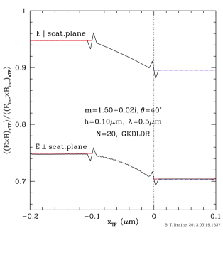
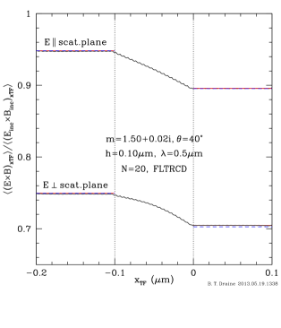
Figure 10: Component of Poynting flux normal to a slab of thickness $h=0.10{\mu{\rm m}}$, refractive index $m=1.5+0.02i$. Radiation with $\lambda/h=5$ is incident with incidence angle $\theta_{i}=40^{\circ}$. The interdipole spacing is set to $d=h/20=0.005{\mu{\rm m}}$. This is the problem considered in Fig. 7b of Draine & Flatau (2008). Left: obtained with DDA method GKDLDR. Right: obtained with DDA method FLTRCD. The red and blue lines show $(1-R)$ for $x_{\rm TF}<-0.1{\mu{\rm m}}$, and $T$ for $x_{\rm TF}>0$, where $R$ and $T$ are the reflection and transmission coefficients. The blue (dashed) lines correspond to the exact solution for $T$ and $R$. The red (solid) line uses the values of $T$ and $R$ computed by DDSCAT 7.3: $T_{\parallel}=S_{11}(\theta_{T})+S_{12}(\theta_{T})$, $R_{\parallel}=S_{11}(\theta_{R})+S_{12}(\theta_{R})$, $T_{\perp}=S_{11}(\theta_{T})-S_{12}(\theta_{T})$, $R_{\perp}=S_{11}(\theta_{R})-S_{12}(\theta_{R})$, with $S_{ij}$ from the output file w000r000k000.sca, $\theta_{T}=40^{\circ}$, and $\theta_{R}=140^{\circ}$.

In Figure 10 we show the component of the time-averaged Poynting flux normal to the slab, $(c/4\pi)\langle({\bf E}\times{\bf B})\rangle\cdot\hat{\bf x}_{\rm TF}$, divided by the time-averaged value of the incident Poynting flux, $(c/8\pi)E_{0}^{2}\cos\theta_{i}$. Figure 10a shows results computed using the standard DDA (method option GKDLDR) and Figure 10b shows results computed using the filtered couple dipole method (option FLTRCD). Both methods give accurate results. The main difference is in the computed ${\bf E}$ field near the surface of the slab: the standard "point dipole" calculation (GKDLDR) has small-scale structure in the computed ${\bf E}$ near the surface, resulting in errors of a few % in the computed Poynting vector near the surface (see Figure 10a). The filtered coupled dipole method, on the other hand, explicitly filters out the small-scale structure in the ${\bf E}$ field, thereby suppressing the "blips" in the Poynting flux near the two surfaces of the slab (see Figure 10b). Otherwise the two solutions are nearly identical, and both are smooth near the middle of the slab.

The numerical accuracy can be assessed from Table 2. For this problem, with $N=20$, both GKDLDR and FLTRCD give reflection and transmission coefficients accurate to better than 0.5%. The absorption coefficients are somewhat less accurate, but the fractional errors do not exceed 4.2%. Note that the filtered coupled dipole method (FLTRCD) does not give greater accuracy than GKDLDR, at least for this problem. If desired, the accuracy could be further improved by increasing $N$.

The CPU time required for the filtered coupled dipole calculations is about twice that required for the GKDLDR method, because for this calculation the dominant calculational task is calculation of the elements of the dipole-dipole interaction matrix (or Green function).

Table 2: Results for $m=1.5+0.02i$, $h/\lambda=0.2$, $\theta_{i}=40^{\circ}$

quantity	exact	GKDLDR	FLTRCD
$R_{\parallel}$	$0.051875$	$0.05179$	$0.051740$
$R_{\perp}$	$0.25046$	$0.25047$	$0.25042$
$T_{\parallel}$	$0.89545$	$0.89534$	$0.89592$
$T_{\perp}$	$0.70280$	$0.70524$	$0.70478$
$A_{\parallel}$	0.052675	$0.052482$	$0.052259$
$A_{\perp}$	0.046748	$0.044970$	$0.044801$
$R_{\parallel}+T_{\parallel}+A_{\parallel}$	1	$0.99961$	$0.99992$
$R_{\perp}+T_{\perp}+A_{\perp}$	1	$1.00068$	$1.00000$
$R_{\parallel}/{\rm exact}-1$	0	$-0.0017$	$-0.0026$
$R_{\perp}/{\rm exact}-1$	0	$+0.0001$	$-0.0002$
$T_{\parallel}/{\rm exact}-1$	0	$-0.0001$	$+0.0005$
$T_{\perp}/{\rm exact}-1$	0	$+0.0035$	$+0.0042$
$A_{\parallel}/{\rm exact}-1$	0	$-0.0037$	$-0.0079$
$A_{\perp}/{\rm exact}-1$	0	$-0.0380$	$-0.0416$
CPU time (s) (2.53GHz Intel, 1 core)	–	1298.	2770.

22.10 RECRECPBC = Rectangular solid resting on top of another rectangular solid, repeated periodically in target y and z directions using periodic boundary conditions

The TUC consists of a single rectangular “brick”, of material 1, resting on top of a second rectangular brick, of material 2. The centroids of the two bricks along a line in the $\hat{\bf x}_{\rm TF}$ direction. The bricks are assumed to be homogeneous, and materials 1 and 2 are assumed to be isotropic. The TUC is then repeated in the $y_{\rm TF}$- and $z_{\rm TF}$-directions, with periodicities SHPAR${}_{4}\times d$ and SHPAR${}_{5}\times d$. is the total volume of solid material in one TUC. This option requires 8 shape parameters:
The pertinent line in ddscat.par should read
 
SHPAR₁ SHPAR₂ SHPAR₃ SHPAR₄ SHPAR₅ SHPAR₆ SHPAR₇ SHPAR₈
 
where
SHPAR₁ = (upper brick thickness)/$d$ in the $\hat{\bf x}_{\rm TF}$ direction
SHPAR₂ = (upper brick thickness)/$d$ in the $\hat{\bf y}_{\rm TF}$ direction
SHPAR₃ = (upper brick thickness)/$d$ in the $\hat{\bf z}_{\rm TF}$ direction
SHPAR₄ = (lower brick thickness)/$d$ in the $\hat{\bf x}_{\rm TF}$ direction
SHPAR₅ = (lower brick thickness)/$d$ in the $\hat{\bf y}_{\rm TF}$ direction
SHPAR₆ = (lower brick thickness)/$d$ in the $\hat{\bf z}_{\rm TF}$ direction
SHPAR₇ = periodicity/$d$ in the $\hat{\bf y}_{\rm TF}$ direction
SHPAR₈ = periodicity/$d$ in the $\hat{\bf z}_{\rm TF}$ direction
 
The actual numbers of dipoles $N_{1x}$, $N_{1y}$, $N_{1z}$, along each dimension of the upper brick, and $N_{2x}$, $N_{2y}$, $N_{2z}$ along each dimension of the lower brick, must be integers. Usually, $N_{1x}={\rm nint}({\tt SHPAR}_{1})$, $N_{1y}={\rm nint}({\tt SHPAR}_{2})$, $N_{1z}={\rm nint}({\tt SHPAR}_{3})$, $N_{2x}={\rm nint}({\tt SHPAR}_{4})$, $N_{2y}={\rm nint}({\tt SHPAR}_{5})$, $N_{2z}={\rm nint}({\tt SHPAR}_{6})$, where ${\rm nint}(x)$ is the integer nearest to $x$, but under some circumstances $N_{1x}$, $N_{1y}$, $N_{1z}$, $N_{2x}$, $N_{2y}$, $N_{2z}$ might be larger or smaller by 1 unit.

The overall size of the TUC (in terms of numbers of dipoles) is determined by parameters SHPAR₁ – SHPAR₆:

$$N=\left(N_{1x}\times N_{1y}\times N_{1z}\right)+\left(N_{2x}\times N_{2y}\times N_{2z}\right)$$ (38)

The physical size of the TUC is specified by the value of ${a}_{\rm eff}$ (in physical units, e.g. cm), specified in the file ddscat.par:

$$d=(4\pi/3N)^{1/3}{a}_{\rm eff}$$ (39)

The periodicity in the $\hat{\bf y}_{\rm TF}$ and $\hat{\bf z}_{\rm TF}$ directions is determined by parameters SHPAR₇ and SHPAR₈.
The periodicity should not be smaller than the extent of the target, so that one should have
 
${\tt SHPAR}_{7}\geq{\rm max}({\tt SHPAR}_{2},{\tt SHPAR}_{5})$
${\tt SHPAR}_{8}\geq{\rm max}({\tt SHPAR}_{3},{\tt SHPAR}_{6})$

The target is a periodic structure, of infinite extent in the $\hat{\bf y}_{\rm TF}$ and $\hat{\bf z}_{\rm TF}$ directions. The target axes are set to ${\hat{\bf a}}_{1}=\hat{\bf x}_{\rm TF}$ – i.e., normal to the “slab” – and ${\hat{\bf a}}_{2}=\hat{\bf y}_{\rm TF}$. The orientation of the incident radiation relative to the target is, as for all other targets, set by the usual orientation angles $\beta$, $\Theta$, and $\Phi$ (see §19 above) specifying the orientation of the target axes ${\hat{\bf a}}_{1}$ and ${\hat{\bf a}}_{2}$ relative to the direction of incidence; for example, $\Theta=0$ would be for radiation incident normal to the slab.

The scattering directions are specified by specifying the diffraction order $(M,N)$; for each diffraction order one transmitted wave direction and one reflected wave direction will be calculated, with the dimensionless $4\times 4$ scattering matrix $S^{(2d)}$ calculated for each scattering direction. At large distances from the infinite slab, the scattered Stokes vector in the (M,N) diffraction order is

$$I_{sca,i}(M,N)=\sum_{j=1}^{4}S_{ij}^{(2d)}I_{in,j}$$ (40)

where $I_{in,j}$ is the incident Stokes vector. See Draine & Flatau (2008) for interpretation of the $S_{ij}$ as transmission and reflection efficiencies.

22.11 SLBHOLPBC = Target consisting of a periodic array of rectangular blocks, each containing a cylindrical hole

Individual blocks have extent $(a,b,c)$ in the $(\hat{\bf x}_{\rm TF},\hat{\bf y}_{\rm TF},\hat{\bf z}_{\rm TF})$ directions, and the cylindrical hole has radius $r$. The period in the $\hat{\bf y}_{\rm TF}$-direction is $P_{y}$, and the period in the $\hat{\bf z}_{\rm TF}$-direction is $P_{z}$.
The pertinent line in ddscat.par should consist of
SHPAR₁ SHPAR₂ SHPAR₃ SHPAR₄ SHPAR₅ SHPAR₆
where SHPAR${}_{1}=a/d$ ($d$ is the interdipole spacing)
SHPAR₂ = $b/a$
SHPAR₃ = $c/a$
SHPAR₄ = $r/a$
SHPAR₅ = $P_{y}/d$
SHPAR₆ = $P_{z}/d$.
Ideally, $a/d=$SHPAR₁, $b/d=$SHPAR${}_{2}\times$SHPAR₁, and $c/d=$SHPAR${}_{3}\times$SHPAR₁ will be integers (so that the cubic lattice can accurately approximate the desired target). If $P_{y}=0$ and $P_{z}>0$ the target is periodic in the $\hat{\bf z}_{\rm TF}$-direction only.
If $P_{y}>0$ and $P_{z}=0$ the target is periodic in the $\hat{\bf y}_{\rm TF}$-direction only.
If $P_{y}>0$ it is required that $P_{y}\geq b$, and if $P_{z}>0$ it is required that $P_{z}\geq c$, so that the blocks do not overlap.
With $P_{y}=b$ and $P_{z}=c$, the blocks are juxtaposed to form a periodic array of cylindrical holes in a solid slab.
Example: ddscat_SLBHOLPBC.par is a sample ddscat.par for a periodic array of cylindrical holes in a slab of thickness $a$, with holes of radius $r$, and period $P_{y}$ and $P_{d}$

22.12 SPHRN_PBC = Target consisting of group of N spheres, extended in target y and z directions using periodic boundary conditions

This option causes DDSCAT to create a target consisting of a periodic array of $N-$sphere structures, where one $N-$sphere structure consists of $N$ spheres, just as for target option NANSPH (see §21.23). Each sphere can be of arbitrary composition, and can be anisotropic if desired. Information for the description of one $N$-sphere structure is supplied via an external file, just as for target option NANSPH – see §21.23).
 
Let us refer to a single $N$-sphere structure as the Target Unit Cell (TUC). The TUC is then repeated in the $y_{\rm TF}$- and $z_{\rm TF}$-directions, with periodicities PYAEFF$\times{a}_{\rm eff}$ and PZAEFF$\times{a}_{\rm eff}$, where ${a}_{\rm eff}\equiv(3V_{\rm TUC}/4\pi)^{1/3}$, where $V_{\rm TUC}$ is the total volume of solid material in one TUC. This option requires 3 shape parameters:
DIAMX = maximum extent of target in the target frame x direction/$d$
PYAEFF = periodicity in target y direction/${a}_{\rm eff}$
PZAEFF = periodicity in target z direction/${a}_{\rm eff}$.

The pertinent line in ddscat.par should read
 
SHPAR₁ SHPAR₂ SHPAR₃ ‘filename’ (quotes must be used)
 
where
SHPAR₁ = target diameter in $x$ direction (in Target Frame) in units of $d$
SHPAR₂= PYAEFF
SHPAR₃= PZAEFF.
filename is the name of the file specifying the locations and relative sizes of the spheres.
 
The overall size of the TUC (in terms of numbers of dipoles) is determined by parameter SHPAR₁, which is the extent of the multisphere target in the $x$-direction, in units of the lattice spacing $d$. The physical size of the TUC is specified by the value of ${a}_{\rm eff}$ (in physical units, e.g. cm), specified in the file ddscat.par.

The location of the spheres in the TUC, and their composition, is specified in file ‘filename’. Please consult §21.23 above for detailed information concerning the information in this file, and its arrangement.

Note that while the spheres can be anisotropic and of differing composition, they can of course also be isotropic and of a single composition, in which case the relevant lines in the file ’filename’ should read
$x_{1}$ $y_{1}$ $z_{1}$ $r_{1}$ 1 1 1 0 0 0
$x_{2}$ $y_{2}$ $z_{2}$ $r_{2}$ 1 1 1 0 0 0
$x_{3}$ $y_{3}$ $z_{3}$ $r_{3}$ 1 1 1 0 0 0
…
i.e., every sphere has isotropic composition ICOMP=1 and the three dielectric function orientation angles are set to zero.

When the user uses target option SPHRN_PBC, the target now becomes a periodic structure, of infinite extent in the target y- and z- directions. The target axis ${\hat{\bf a}}_{1}=\hat{\bf x}_{\rm LF}=(1,0,0)_{\rm TF}$ – i.e., normal to the “slab” – and target axis ${\hat{\bf a}}_{2}=\hat{\bf y}_{\rm LF}=(0,1,0)_{\rm TF}$. The orientation of the incident radiation relative to the target is, as for all other targets, set by the usual orientation angles $\beta$, $\Theta$, and $\Phi$ (see §19 above). The scattering directions are, just as for other targets, determined by the scattering angles $\theta_{s}$, $\phi_{s}$ (see §23 below).

The scattering problem for this infinite structure, assumed to be illuminated by an incident monochromatic plane wave, is essentially solved “exactly”, in the sense that the electric polarization of each of the constituent dipoles is due to the electric field produced by the incident plane wave plus all of the other dipoles in the infinite target.

However, the assumed target will, of course, act as a perfect diffraction grating if the scattered radiation is calculated as the coherent sum of all the oscillating dipoles in this periodic structure: the far-field scattered intensity would be zero in all directions except those where the Bragg scattering condition is satisfied, and in those directions the far-field scattering intensity would be infinite.

To suppress this singular behavior, we calculate the far-field scattered intensity as though the separate TUCs scatter incoherently. The scattering efficiency $Q_{\rm sca}$ and the absorption efficiency $Q_{\rm abs}$ are defined to be the scattering and absorption cross section per TUC, divided by $\pi{a}_{\rm eff}^{2}$, where ${a}_{\rm eff}\equiv(3V_{\rm TUC}/4\pi)^{1/3}$, where $V_{\rm TUC}$ is the volume of solid material per TUC.

Note: the user is allowed to set the target periodicity in the target $y_{\rm TF}$ (or $z_{\rm TF}$) direction to values that could be smaller than the total extent of one TUC in the target $y_{\rm TF}$ (or $z_{\rm TF}$) direction. This is physically allowable, provided that the spheres from one TUC do not overlap with the spheres from neighboring TUCs. Note that DDSCAT does not check for such overlap.

22.12.1 Sample calculation in directory examples_exp/SPHRN_PBC

Subdirectory examples_exp/SPHRN_PBC contains ddscat.par to calculate scattering by a doubly-periodic array with the target unit cell consisting of a random cluster of 16 spheres. The calculation is carried out with double precision arithmetic. Because convergence is slow, the error tolerance is set to TOL = 5.e-5 rather than the usual 1.e-5, and the maximum number of iterations allowed is increased to MXITER = 2000.

22.13 TRILYRPBC = Three stacked rectangular blocks, repeated periodically

The target unit cell (TUC) consists of a stack of 3 rectangular blocks with centers on the $\hat{\bf x}_{\rm TF}$ axis. The TUC is repeated in either the $\hat{\bf y}_{\rm TF}$ direction, the $\hat{\bf z}_{\rm TF}$ direction, or both. A total of 11 shape parameters must be specified:
SHPAR₁ = x-thickness of upper layer/$d$ [material 1]
SHPAR₂ = y-width/$d$ of upper layer
SHPAR₃ = z-width/$d$ of upper layer
SHPAR₄ = x-thickness/$d$ of middle layer [material 2]
SHPAR₅ = y-width/$d$ of middle layer
SHPAR₆ = z-width/$d$ of middle layer
SHPAR₇ = x-width/$d$ of lower layer
SHPAR₈ = y-width/$d$ of lower layer
SHPAR₉ = z-width/$d$ of lower layer
SHPAR₁₀ = period/$d$ in y direction
SHPAR₁₁= period/$d$ in z direction

23 Scattering Directions

23.1 Isolated Finite Targets

DDSCAT calculates scattering in selected directions, and elements of the scattering matrix are reported in the output files wxxxryyykzzz.sca . The scattering direction is specified through angles $\theta_{s}$ and $\phi_{s}$ (not to be confused with the angles $\Theta$ and $\Phi$ which specify the orientation of the target relative to the incident radiation!).

For isolated finite targets (i.e., PBC not employed) there are two options for specifying the scattering direction, with the option determined by the value of the string CMDFRM read from the input file ddscat.par.

1. If the user specifies CMDFRM=’LFRAME’, then the angles $\theta$, $\phi$ input from ddscat.par are understood to specify the scattering directions relative to the Lab Frame (the frame where the incident beam is in the $x-$direction).

   When CMDFRM=’LFRAME’, the angle $\theta$ is simply the scattering angle $\theta_{s}$: the angle between the incident beam (in direction $\hat{\bf x}_{\rm LF}$) and the scattered beam ($\theta_{s}=0$ for forward scattering, $\theta_{s}=180^{\circ}$ for backscattering).

   The angle $\phi$ specifies the orientation of the “scattering plane” relative to the $\hat{\bf x}_{\rm LF}-\hat{\bf y}_{\rm LF}$ plane. When $\phi=0$ the scattering plane is assumed to coincide with the $\hat{\bf x}_{\rm LF}-\hat{\bf y}_{\rm LF}$ plane. When $\phi=90^{\circ}$ the scattering plane is assumed to coincide with the ${\hat{\bf x}_{\rm LF}-\hat{\bf z}_{\rm LF}}$ plane. Within the scattering plane the scattering directions are specified by $0\leq\theta\leq 180^{\circ}$. Thus:

   $$\hat{\bf n}_{s}=\hat{\bf x}_{\rm LF}\cos\theta+\hat{\bf y}_{\rm LF}\sin\theta\cos\phi+\hat{\bf z}_{\rm LF}\sin\theta\sin\phi\leavevmode\nobreak\ \leavevmode\nobreak\ \leavevmode\nobreak\ ,\leavevmode\nobreak\ \leavevmode\nobreak\ \leavevmode\nobreak\$$ (41)

2. If the user specifies CMDFRM=’TFRAME’, then the angles $\theta$, $\phi$ input from ddscat.par are understood to specify the scattering directions $\bf\hat{n}_{s}$ relative to the Target Frame (the frame defined by target axes $\hat{\bf x}_{\rm TF}$, $\hat{\bf y}_{\rm TF}$, $\hat{\bf z}_{\rm TF}$). $\theta$ is the angle between $\hat{\bf n}_{s}$ and $\hat{\bf x}_{\rm TF}$, and $\phi$ is the angle between the $\hat{\bf n}_{s}-\hat{\bf x}_{\rm TF}$ plane and the $\hat{\bf x}_{\rm TF}-\hat{\bf y}_{\rm TF}$ plane. Thus:

   $$\hat{\bf n}_{s}=\hat{\bf x}_{\rm TF}\cos\theta+\hat{\bf y}_{\rm TF}\sin\theta\cos\phi+\hat{\bf z}_{\rm TF}\sin\theta\sin\phi\leavevmode\nobreak\ \leavevmode\nobreak\ \leavevmode\nobreak\ .\leavevmode\nobreak\ \leavevmode\nobreak\ \leavevmode\nobreak\$$ (42)

Scattering directions for which the scattering properties are to be calculated are set in the parameter file ddscat.par by specifying one or more scattering planes (determined by the value of $\phi_{s}$) and for each scattering plane, the number and range of $\theta_{s}$ values. The only limitation is that the number of scattering directions not exceed the parameter MXSCA in DDSCAT.f (in the code as distributed it is set to MXSCA=1000).

23.2 Scattering Directions for Targets that are Periodic in 1 Dimension

For targets that are periodic, scattering is only allowed in certain directions (Draine & Flatau 2008, see). If the user has chosen a PBC target (e.g, CYLNDRPBC, HEXGONPBC, or RCTGL_PBC), SPHRN_PBC but has set one of the periodicities to zero, then the target is periodic in only one dimension – e.g., CYLNDRPBC could be used to construct a single infinite cylinder.

In this case, the scattering directions are specified by giving an integral diffraction order $M=0,\pm 1,\pm 2,...$ and one angle, the azimuthal angle $\zeta$ around the target repetition axis. The diffraction order $M$ determines the projection of ${\bf k}_{s}$ onto the repetition direction. For a given order $M$, the scattering angles with $\zeta=0\rightarrow 2\pi$ form a cone around the repetition direction.

For example, if ${\tt PYD}>0$ (target repeating in the $y_{\rm TF}$ direction), then $M$ determines the value of $k_{sy}={\bf k}_{s}\cdot\hat{\bf y}_{\rm TF}$, where $\hat{\bf y}_{\rm TF}$ is the unit vector in the Target Frame $y-$direction:

$$k_{sy}=k_{0y}+2\pi M/L_{y}$$ (43)

where $k_{0y}\equiv{\bf k}_{0}\cdot\hat{\bf y}_{\rm TF}$, where ${\bf k}_{0}$ is the incident $k$ vector. Note that the diffraction order $M$ must satisfy the condition

$$(k_{0y}-k_{0})(L_{y}/2\pi)<M<(k_{0}-k_{0y})(L_{y}/2\pi)$$ (44)

where $L_{y}={\tt PYD}\times d$ is the periodicity along the $y$ axis in the Target Frame. $M=0$ is always an allowed diffraction order.

The azimuthal angle $\zeta$ defines a right-handed rotation of the scattering direction around the target repetition axis. Thus for a target repetition axis $\hat{\bf y}_{\rm TF}$,

$$k_{sx} = k_{\perp}\cos\zeta\leavevmode\nobreak\ \leavevmode\nobreak\ \leavevmode\nobreak\ ,$$ (45)

$$k_{sz} = k_{\perp}\sin\zeta\leavevmode\nobreak\ \leavevmode\nobreak\ \leavevmode\nobreak\ ,$$ (46)

where $k_{\perp}=(k_{0}^{2}-k_{sy}^{2})^{1/2}$, with $k_{sy}=k_{0y}+2\pi M/L_{y}$. For a target with repetition axis $z_{\rm TF}$,

$$k_{sx} = k_{\perp}\cos\zeta\leavevmode\nobreak\ \leavevmode\nobreak\ \leavevmode\nobreak\ ,$$ (47)

$$k_{sy} = k_{\perp}\sin\zeta\leavevmode\nobreak\ \leavevmode\nobreak\ \leavevmode\nobreak\ ,$$ (48)

where $k_{\perp}=(k_{0}^{2}-k_{sz}^{2})^{1/2}$, $k_{sz}=k_{0z}+2\pi M/L_{z}$.

The user selects a diffraction order $M$ and the azimuthal angles $\zeta$ to be used for that $M$ via one line in ddscat.par. An example would be to use CYLNDRPBC to construct an infinite cylinder with the cylinder direction in the $\hat{\bf y}_{\rm TF}$ direction: e.g., examples_exp/CYLNDRPBC/ddscat.par :

’ ========== Parameter file for v7.3 ===================’
’**** Preliminaries ****’
’NOTORQ’ = CMTORQ*6 (DOTORQ, NOTORQ) -- either do or skip torque calculations
’PBCGS2’ = CMDSOL*6 (PBCGS2, PBCGST, GPBICG, QMRCCG, PETRKP) -- CCG method
’GPFAFT’ = CMETHD*6 (GPFAFT, FFTMKL) -- FFT method
’GKDLDR’ = CALPHA*6 (GKDLDR, LATTDR, FLTRCD) -- DDA method
’NOTBIN’ = CBINFLAG (NOTBIN, ORIGIN, ALLBIN)
’**** Initial Memory Allocation ****’
100 100 100 = dimensioning allowance for target generation
’**** Target Geometry and Composition ****’
’CYLNDRPBC’ = CSHAPE*9 shape directive
1 64.499 2 1.0 0.0  = shape parameters 1 - 7
1         = NCOMP = number of dielectric materials
’../diel/m1.33_0.01’ = file with refractive index 1
’**** Additional Nearfield calculation? ****’
0 = NRFLD (=0 to skip nearfield calc., =1 to calculate nearfield E)
0.0 0.0 0.0 0.0 0.0 0.0 (fract. extens. of calc. vol. in -x,+x,-y,+y,-z,+z)
’**** Error Tolerance ****’
1.00e-5 = TOL = MAX ALLOWED (NORM OF |G>=AC|E>-ACA|X>)/(NORM OF AC|E>)
’**** Maximum number of iterations ****’
200      = MXITER
’**** Integration limiter for PBC calculations ****’
1.00e-3 = GAMMA (1e-2 is normal, 3e-3 for greater accuracy)
’**** Angular resolution for calculation of <cos>, etc. ****’
0.5Ψ= ETASCA (number of angles is proportional to [(3+x)/ETASCA]^2 )
’**** Vacuum wavelengths (micron) ****’
6.283185 6.283185 1 ’LIN’ = wavelengths (first,last,how many,how=LIN,INV,LOG)
’**** Refractive index of ambient medium’
1.0000 = NAMBIENT
’**** Effective Radii (micron) **** ’
2.8555 2.8555 1 ’LIN’ = aeff (first,last,how many,how=LIN,INV,LOG)
’**** Define Incident Polarizations ****’
(0,0) (1.,0.) (0.,0.) = Polarization state e01 (k along x axis)
2 = IORTH  (=1 to do only pol. state e01; =2 to also do orth. pol. state)
’**** Specify which output files to write ****’
1 = IWRKSC (=0 to suppress, =1 to write ".sca" file for each target orient.
’**** Specify Target Rotations ****’
0.    0.   1  = BETAMI, BETAMX, NBETA  (beta=rotation around a1)
60.  60.   1  = THETMI, THETMX, NTHETA (theta=angle between a1 and k)
0.    0.   1  = PHIMIN, PHIMAX, NPHI (phi=rotation angle of a1 around k)
’**** Specify first IWAV, IRAD, IORI (normally 0 0 0) ****’
0   0   0    = first IWAV, first IRAD, first IORI (0 0 0 to begin fresh)
’**** Select Elements of S_ij Matrix to Print ****’
6Ψ= NSMELTS = number of elements of S_ij to print (not more than 9)
11 12 21 22 31 41Ψ= indices ij of elements to print
’**** Specify Scattered Directions ****’
’TFRAME’ = CMDFRM (LFRAME, TFRAME for Lab Frame or Target Frame)
1 = NPLANES = number of scattering cones
0.  0. 180. 1  = OrderM zetamin zetamax dzeta for scattering cone 1

In this example, a single diffraction order $M=0$ is selected, and $\zeta$ is to run from $\zeta_{\rm min}=0$ to $\zeta_{\rm max}=180^{\circ}$ in increments of $\delta\zeta=0.05^{\circ}$.

There may be additional lines, one per diffraction order. Remember, however, that every diffraction order must satisfy eq. (44).

23.3 Scattering Directions for Targets for Doubly-Periodic Targets

If the user has specified nonzero periodicity in both the $y$ and $z$ directions, then the scattering directions are specified by two integers – the diffraction orders $M,N$ for the $\hat{\bf y},\hat{\bf z}$ directions. The scattering directions are

$${\bf k}_{s}=\pm\,\frac{k_{n}}{k_{0}}\left({\bf k}_{0}\cdot\hat{\bf x}_{\rm TF}\right)\hat{\bf x}_{\rm TF}+\left({\bf k}_{0}\cdot\hat{\bf y}_{\rm TF}+\frac{2\pi M}{L_{y}}\right)\hat{\bf y}_{\rm TF}+\left({\bf k}_{0}\cdot\hat{\bf z}_{\rm TF}+\frac{2\pi N}{L_{z}}\right)\hat{\bf z}_{\rm TF}$$ (49)

$$k_{n}\equiv\left[k_{0}^{2}-\left({\bf k}_{0}\cdot\hat{\bf y}_{\rm TF}+\frac{2\pi M}{L_{y}}\right)^{2}+\left({\bf k}_{0}\cdot\hat{\bf z}_{\rm TF}+\frac{2\pi N}{L_{z}}\right)^{2}\right]^{1/2}$$ (50)

where the $+$ sign gives transmission, and the $-$ sign gives reflection. The integers $M$ and $N$ must together satisfy the inequality

$$({\bf k}_{0}\cdot\hat{\bf y}_{\rm TF}+2\pi M/L_{y})^{2}+({\bf k}_{0}\cdot\hat{\bf z}_{\rm TF}+2\pi N/L_{z})^{2}<k_{0}^{2}$$ (51)

which, for small values of $L_{y}$ and $L_{z}$, may limit the scattering to only $(M,N)=(0,0)$. [Of course, $(0,0)$ is always allowed]. For each $(M,N)$ specified in ddscat.par, DDSCAT 7.3 will calculate the generalized Mueller matrix $S_{ij}^{(2d)}(M,N)$ – see §27.2. At large distances from the infinite slab, the scattered Stokes vector in the $(M,N)$ diffraction order is

$$I_{sca,i}(M,N)=\sum_{j=1}^{4}S_{ij}^{(2d)}(M,N)I_{in,j}$$ (52)

where $I_{in,j}$ is the incident Stokes vector, and $S_{ij}^{(2d)}(M,N)$ is the generalization of the $4\times 4$ Müller scattering matrix to targets that are periodic in 2-directions (Draine & Flatau 2008). There are distinct $S_{ij}^{(2d)}(M,N)$ for transmission and for reflection, corresponding to the $\pm$ in eq. (49).

Draine & Flatau (2008) (eq. 69-71) show how the $S_{ij}^{(2d)}(M,N)$ are easily related to familiar "transmission coefficients" and "reflection coefficients".

Here is examples_exp/RCTGL_PBC/ddscat.par file as an example:

’ =========== Parameter file for v7.3 ===================’
’**** Preliminaries ****’
’NOTORQ’ = CMTORQ*6 (DOTORQ, NOTORQ) -- either do or skip torque calculations
’PBCGS2’ = CMDSOL*6 (PBCGS2,PBCGST, GPBICG, QMRCCG, PETRKP) -- CCG method
’GPFAFT’ = CMDFFT*6 (GPFAFT, FFTMKL) -- FFT method
’GKDLDR’ = CALPHA*6 (GKDLDR, LATTDR, FLTRCD) -- DDA method
’NOTBIN’ = CBINFLAG (NOTBIN, ORIBIN, ALLBIN)
’**** Initial Memory Allocation ****’
100 100 100 = dimensioning allowance for target generation
’**** Target Geometry and Composition ****’
’RCTGL_PBC’ = CSHAPE*9 shape directive
20 1 1 1 1 = shpar1 - shpar5 (see README.txt)
1         = NCOMP = number of dielectric materials
’../diel/m1.50_0.02’    = refractive index 1
’**** Additional Nearfield calculation? ****’
0 = NRFLD (=0 to skip nearfield calc., =1 to calculate nearfield E)
0.0 0.0 0.0 0.0 0.0 0.0 (fract. extens. of calc. vol. in -x,+x,-y,+y,-z,+z)
’**** Error Tolerance ****’
1.00e-5 = TOL = MAX ALLOWED (NORM OF |G>=AC|E>-ACA|X>)/(NORM OF AC|E>)
’**** Maximum number of iterations ****’
100      = MXITER
’**** Integration limiter for PBC calculations ****’
1.00e-2 = GAMMA (1e-2 is normal, 3e-3 for greater accuracy)
’**** Angular resolution for calculation of <cos>, etc. ****’
1.Ψ= ETASCA (number of angles is proportional to [(3+x)/ETASCA]^2 )
’**** Vacuum wavelengths (micron) ****’
0.5 0.5 1 ’LIN’ = wavelengths (first,last,how many,how=LIN,INV,LOG)
’**** Refractive index of ambient medium’
1.000 = NAMBIENT
’**** Effective Radii (micron) **** ’
0.0084195 0.0084195 1 ’LIN’ = aeff (first,last,how many,how=LIN,INV,LOG)
’**** Define Incident Polarizations ****’
(0,0) (1.,0.) (0.,0.) = Polarization state e01 (k along x axis)
2 = IORTH  (=1 to do only pol. state e01; =2 to also do orth. pol. state)
’**** Specify which output files to write ****’
1 = IWRKSC (=0 to suppress, =1 to write ".sca" file for each target orient.
’**** Prescribe Target Rotations ****’
0.   0.   1  = BETAMI, BETAMX, NBETA (beta=rotation around a1)
40. 40.   1  = THETMI, THETMX, NTHETA (theta=angle between a1 and k)
0.   0.   1  = PHIMIN, PHIMAX, NPHI (phi=rotation angle of a1 around k)
’**** Specify first IWAV, IRAD, IORI (normally 0 0 0) ****’
0   0   0    = first IWAV, first IRAD, first IORI (0 0 0 to begin fresh)
’**** Select Elements of S_ij Matrix to Print ****’
6       = NSMELTS = number of elements of S_ij to print (not more than 9)
11 12 21 22 31 41       = indices ij of elements to print
’**** Specify Scattered Directions ****’
’TFRAME’ = CMDFRM (LFRAME, TFRAME for Lab Frame or Target Frame)
1 = NORDERS = number of diffraction orders for transmission
0. 0.

24 Incident Polarization State

Recall that the “Lab Frame” is defined such that the incident radiation is propagating along the $\hat{\bf x}_{\rm LF}$ axis. DDSCAT allows the user to specify a general elliptical polarization for the incident radiation, by specifying the (complex) polarization vector ${\hat{\bf e}}_{01}$. The orthonormal polarization state ${\hat{\bf e}}_{02}=\hat{\bf x}_{\rm LF}\times{\hat{\bf e}}_{01}^{*}$ is generated automatically if ddscat.par specifies IORTH=2.

For incident linear polarization, one can simply set ${\hat{\bf e}}_{01}={\hat{\bf y}}$ by specifying
(0,0) (1,0) (0,0)
in ddscat.par; then ${\hat{\bf e}}_{02}={\hat{\bf z}}$. For polarization mode ${\hat{\bf e}}_{01}$ to correspond to right-handed circular polarization, set ${\hat{\bf e}}_{01}=({\hat{\bf y}}+i{\hat{\bf z}})/\surd 2$ by specifying (0,0) (1,0) (0,1) in ddscat.par (DDSCAT automatically takes care of the normalization of ${\hat{\bf e}}_{01}$); then ${\hat{\bf e}}_{02}=(i{\hat{\bf y}}+{\hat{\bf z}})/\surd 2$, corresponding to left-handed circular polarization.

25 Averaging over Scattering Directions: $g(1)=\langle\cos\theta_{s}\rangle$, etc.

25.1 Angular Averaging

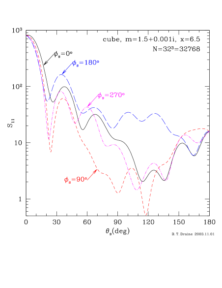
Figure 11: Scattered intensity for incident unpolarized light for a cube with $m=1.5+0.001i$ and $x=2\pi a_{\rm eff}/\lambda=6.5$ (i.e., $d/\lambda=1.6676$, where $d$ is the length of a side). The cube is tilted with respect to the incident radiation, with $\Theta=30^{\circ}$, and rotated by $\beta=15^{\circ}$ around its axis to break reflection symmetry. The Mueller matrix element $S_{11}$ is shown for 4 different scattering planes. The strong forward scattering lobe is evident. It is also seen that the scattered intensity is a strong function of scattering angle $\phi_{s}$ as well as $\theta_{s}$ – at a given value of $\theta_{s}$ (e.g., $\theta_{s}=120^{\circ}$), the scattered intensity can vary by orders of magnitude as $\phi_{s}$ changes by $90^{\circ}$.

An example of scattering by a nonspherical target is shown in Fig. 11, showing the scattering for a tilted cube. Results are shown for four different scattering planes.

DDSCAT automatically carries out numerical integration of various scattering properties, including

• $\langle\cos\theta_{s}\rangle$;

• $\langle\cos^{2}\theta_{s}\rangle$;

• ${\bf g}=\langle\cos\theta_{s}\rangle\hat{\bf x}_{\rm LF}+\langle\sin\theta_{s}\cos\phi_{s}\rangle{\hat{\bf y}}+\langle\sin\theta_{s}\sin\phi_{s}\rangle{\hat{\bf z}}\leavevmode\nobreak\$ (see §16);

• ${\bf Q}_{\Gamma}$, provided option DOTORQ is specified (see §16).

The angular averages are accomplished by evaluating the scattered intensity for selected scattering directions $(\theta_{s},\phi_{s})$, and taking the appropriately weighted sum. Suppose that we have $N_{\theta}$ different values of $\theta_{s}$,

$$\theta=\theta_{j},\leavevmode\nobreak\ \leavevmode\nobreak\ \leavevmode\nobreak\ j=1,...,N_{\theta}\leavevmode\nobreak\ \leavevmode\nobreak\ \leavevmode\nobreak\ ,$$ (53)

and for each value of $\theta_{j}$, $N_{\phi}(j)$ different values of $\phi_{s}$:

$$\phi_{s}=\phi_{j,k},\leavevmode\nobreak\ \leavevmode\nobreak\ \leavevmode\nobreak\ k=1,...,N_{\phi}(j)\leavevmode\nobreak\ \leavevmode\nobreak\ \leavevmode\nobreak\ .$$ (54)

For a given $j$, the values of $\phi_{j,k}$ are assumed to be uniformly spaced: $\phi_{j,k+1}-\phi_{j,k}=2\pi/N_{\phi}(j)$. The angular average of a quantity $f(\theta_{s},\phi_{s})$ is approximated by

$$\langle f\rangle\equiv\frac{1}{4\pi}\int_{0}^{\pi}\sin\theta_{s}d\theta_{s}\int_{0}^{2\pi}d\phi_{s}f(\theta_{s},\phi_{s})\leavevmode\nobreak\ \approx\leavevmode\nobreak\ \frac{1}{4\pi}\sum_{j=1}^{N_{\theta}}\sum_{k=1}^{N_{\phi}(j)}f(\theta_{j},\phi_{j,k})\Omega_{j,k}$$ (55)

$$\Omega_{j,k}=\frac{\pi}{N_{\phi}(j)}\left[\cos(\theta_{j-1})-\cos(\theta_{j+1})\right]\leavevmode\nobreak\ \leavevmode\nobreak\ \leavevmode\nobreak\ ,\leavevmode\nobreak\ \leavevmode\nobreak\ \leavevmode\nobreak\ j=2,...,N_{\theta}-1\leavevmode\nobreak\ \leavevmode\nobreak\ \leavevmode\nobreak\ .$$ (56)

$$\Omega_{1,k}=\frac{2\pi}{N_{\phi}(1)}\left[1-\frac{\cos(\theta_{1})+\cos(\theta_{2})}{2}\right]\leavevmode\nobreak\ \leavevmode\nobreak\ \leavevmode\nobreak\ ,$$ (57)

$$\Omega_{N_{\theta},k}=\frac{2\pi}{N_{\phi}(N_{\theta})}\left[\frac{\cos(\theta_{N_{\theta}-1})+\cos(\theta_{N_{\theta}})}{2}+1\right]\leavevmode\nobreak\ \leavevmode\nobreak\ \leavevmode\nobreak\ .$$ (58)

For a sufficiently large number of scattering directions

$$N_{\rm sca}\equiv\sum_{j=1}^{N_{\theta}}N_{\phi}(j)$$ (59)

the sum (55) approaches the desired integral, but the calculations can be a significant cpu-time burden, so efficiency is an important consideration.

25.2 Selection of Scattering Angles $\theta_{s},\phi_{s}$

Beginning with DDSCAT 6.1, an improved approach is taken to evaluation of the angular average. Since targets with large values of $x=2\pi a_{\rm eff}/\lambda$ in general have strong forward scattering, it is important to obtain good sampling of the forward scattering direction. To implement a preferential sampling of the forward scattering directions, the scattering directions $(\theta,\phi)$ are chosen so that $\theta$ values correspond to equal intervals in a monotonically increasing function $s(\theta)$. The function $s(\theta)$ is chosen to have a negative second derivative $d^{2}s/d\theta^{2}<0$ so that the density of scattering directions will be higher for small values of $\theta$. DDSCAT takes

$$s(\theta)=\theta+\frac{\theta}{\theta+\theta_{0}}\leavevmode\nobreak\ \leavevmode\nobreak\ \leavevmode\nobreak\ .$$ (60)

This provides increased resolution (i.e., increased $ds/d\theta$) for $\theta<\theta_{0}$. We want this for the forward scattering lobe, so we take

$$\theta_{0}=\frac{2\pi}{1+x}\leavevmode\nobreak\ \leavevmode\nobreak\ .$$ (61)

The $\theta$ values run from $\theta=0$ to $\theta=\pi$, corresponding to uniform increments

$$\Delta s=\frac{1}{N_{\theta}-1}\left(\pi+\frac{\pi}{\pi+\theta_{0}}\right)\leavevmode\nobreak\ \leavevmode\nobreak\ \leavevmode\nobreak\ .$$ (62)

If we now require that

$$\max[\Delta\theta]\approx\frac{\Delta s}{(ds/d\theta)_{\theta=\pi}}=\eta\frac{\pi/2}{3+x}\leavevmode\nobreak\ \leavevmode\nobreak\ \leavevmode\nobreak\ ,$$ (63)

we determine the number of values of $\theta$:

$$N_{\theta}=1+\frac{2(3+x)}{\eta}\frac{\left[1+1/(\pi+\theta_{0})\right]}{\left[1+\theta_{0}/(\pi+\theta_{0})^{2}\right]}\leavevmode\nobreak\ \leavevmode\nobreak\ \leavevmode\nobreak\ .$$ (64)

Thus for small values of $x$, $\max[\Delta\theta]=30^{\circ}\eta$, and for $x\gg 1$, $\max[\Delta\theta]\rightarrow 90^{\circ}\eta/x$. For a sphere, minima in the scattering pattern are separated by $\sim 180^{\circ}/x$, so $\eta=1$ would be expected to marginally resolve structure in the scattering function. Smaller values of $\eta$ will obviously lead to improved sampling of the scattering function, and more accurate angular averages.

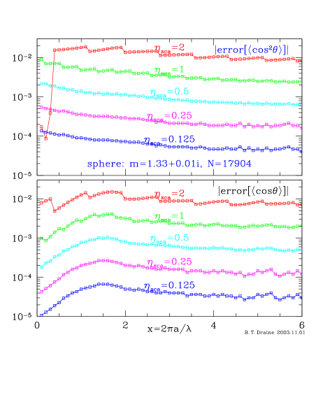
Figure 12: Errors in $\langle\cos\theta\rangle$ and $\langle\cos^{2}\theta\rangle$ calculated for a $N=17904$ dipole pseudosphere with $m=1.33+0.01i$, as functions of $x=2\pi a/\lambda$. Results are shown for different values of the parameter $\eta$.

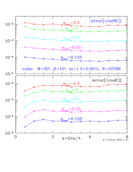
Figure 13: Same as Fig. 12, but for a $N=32768$ dipole cube with $m=1.5+0.001i$.

The scattering angles $\theta_{j}$ used for the angular averaging are then given by

$$\theta_{j}=\frac{(s_{j}-1-\theta_{0})+\left[(1+\theta_{0}-s_{j})^{2}+4\theta_{0}s_{j}\right]^{1/2}}{2}\leavevmode\nobreak\ \leavevmode\nobreak\ \leavevmode\nobreak\ ,$$ (65)

where

$$s_{j}=\frac{(j-1)\pi}{N_{\theta}-1}\left[1+\frac{1}{\pi+\theta_{0}}\right]\leavevmode\nobreak\ \leavevmode\nobreak\ \leavevmode\nobreak\ j=1,...,N_{\theta}\leavevmode\nobreak\ \leavevmode\nobreak\ \leavevmode\nobreak\ .$$ (66)

For each $\theta_{j}$, we must choose values of $\phi$. For $\theta_{1}=0$ and $\theta_{N_{\theta}}=\pi$ only a single value of $\phi$ is needed (the scattering is independent of $\phi$ in these two directions). For $0<\theta_{j}<\pi$ we use

$$N_{\phi}=\max\left\{3,{\rm nint}\left[4\pi\sin(\theta_{j})/(\theta_{j+1}-\theta_{j-1})\right]\right\}\leavevmode\nobreak\ \leavevmode\nobreak\ \leavevmode\nobreak\ ,$$ (67)

where ${\rm nint}=$ nearest integer. This provides sampling in $\phi$ consistent with the sampling in $\theta$.

25.3 Accuracy of Angular Averaging as a Function of $\eta$

Figure 12 shows the absolute errors in $\langle\cos\theta\rangle$ and $\langle\cos^{2}\theta\rangle$ calculated for a sphere with refractive index $m=1.33+0.01i$ using the above prescription for choosing scattering angles. The error is shown as a function of scattering parameter $x$. We see that accuracies of order 0.01 are attained with $\eta=1$, and that the above prescription provides an accuracy which is approximately independent of $x$. We recommend using values of $\eta\leq 1$ unless accuracy in the angular averages is not important.

26 Scattering by Finite Targets: The Mueller Matrix

26.1 Two Orthogonal Incident Polarizations (IORTH=2)

Subsection 26.1 is intended for those studying the internals of DDSCAT to see how it obtains the elements of the scattering amplitude matrix (see Bohren & Huffman 1983)

$$\left(\begin{array}[]{c c}S_{2}&S_{3}\\ S_{4}&S_{1}\end{array}\right)\leavevmode\nobreak\ \leavevmode\nobreak\ \leavevmode\nobreak\ .$$ (68)

Unless you are interested in such computational details, you can skip this subsection and go forward to §26.2.

Throughout the following discussion, $\hat{\bf x}_{\rm LF}$, $\hat{\bf y}_{\rm LF}$, $\hat{\bf z}_{\rm LF}$ are unit vectors defining the Lab Frame (thus $\hat{\bf k}_{0}=\hat{\bf x}_{\rm LF}$).

DDSCAT internally computes the scattering properties of the dipole array in terms of a complex scattering matrix $f_{ml}(\theta_{s},\phi_{s})$ (Draine 1988), where index $l=1,2$ denotes the incident polarization state, $m=1,2$ denotes the scattered polarization state, and $\theta_{s}$,$\phi_{s}$ specify the scattering direction. Normally DDSCAT is used with IORTH=2 in ddscat.par, so that the scattering problem will be solved for both incident polarization states ($l=1$ and 2); in this subsection it will be assumed that this is the case.

Incident polarization states $l=1,2$ correspond to polarization states ${\hat{\bf e}}_{01}$, ${\hat{\bf e}}_{02}$; recall that polarization state ${\hat{\bf e}}_{01}$ is user-specified, and ${\hat{\bf e}}_{02}=\hat{\bf k}_{0}\times{\hat{\bf e}}_{01}^{*}=\hat{\bf x}_{\rm LF}\times{\hat{\bf e}}_{01}^{*}$.^, In the DDSCAT code, which follows the convention in Draine (1988), scattered polarization state $m=1$ corresponds to linear polarization of the scattered wave parallel to the scattering plane (${\hat{\bf e}}_{1}={\hat{\bf e}}_{\parallel s}=\hat{\theta}_{s}$) and $m=2$ corresponds to linear polarization perpendicular to the scattering plane (in the $+\hat{\phi}_{s}$ direction: $\hat{\bf e}_{2}=\hat{\phi}_{s}$). The scattering matrix $f_{ml}$ was defined (Draine 1988) so that the scattered electric field ${\bf E}_{s}$ is related to the incident electric field ${\bf E}_{i}(0)$ at the origin (where the target is assumed to be located) by

$$\left(\begin{array}[]{c}{\bf E}_{s}\cdot\hat{\theta}_{s}\\ {\bf E}_{s}\cdot\hat{\phi}_{s}\end{array}\right)={\exp(i{\bf k}_{s}\cdot{\bf r})\over kr}\left(\begin{array}[]{cc}f_{11}&f_{12}\\ f_{21}&f_{22}\end{array}\right)\left(\begin{array}[]{c}{\bf E}_{i}(0)\cdot{\hat{\bf e}}_{01}^{*}\\ {\bf E}_{i}(0)\cdot{\hat{\bf e}}_{02}^{*}\end{array}\right)\leavevmode\nobreak\ \leavevmode\nobreak\ \leavevmode\nobreak\ .$$ (69)

The 2$\times$2 complex scattering amplitude matrix (with elements $S_{1}$, $S_{2}$, $S_{3}$, and $S_{4}$) is defined so that (see Bohren & Huffman 1983)

$$\left(\begin{array}[]{c}{\bf E}_{s}\cdot\hat{\theta}_{s}\\ -{\bf E}_{s}\cdot\hat{\phi}_{s}\end{array}\right)={\exp(i{\bf k}_{s}\cdot{\bf r})\over-ikr}\left(\begin{array}[]{cc}S_{2}&S_{3}\\ S_{4}&S_{1}\end{array}\right)\left(\begin{array}[]{c}{\bf E}_{i}(0)\cdot{\hat{\bf e}}_{i\parallel}\\ {\bf E}_{i}(0)\cdot{\hat{\bf e}}_{i\perp}\end{array}\right)\leavevmode\nobreak\ \leavevmode\nobreak\ \leavevmode\nobreak\ ,$$ (70)

where ${\hat{\bf e}}_{i\parallel}$, ${\hat{\bf e}}_{i\perp}$ are (real) unit vectors for incident polarization parallel and perpendicular to the scattering plane (with the customary definition of ${\hat{\bf e}}_{i\perp}={\hat{\bf e}}_{i\parallel}\times\hat{\bf k}_{0}={\hat{\bf e}}_{i\parallel}\times{\hat{\bf x}_{\rm LF}}$).

From (69,70) we may write

$$\left(\begin{array}[]{cc}S_{2}&S_{3}\\ S_{4}&S_{1}\end{array}\right)\left(\begin{array}[]{c}{\bf E}_{i}(0)\cdot{\hat{\bf e}}_{i\parallel}\\ {\bf E}_{i}(0)\cdot{\hat{\bf e}}_{i\perp}\end{array}\right)=-i\left(\begin{array}[]{cc}f_{11}&f_{12}\\ -f_{21}&-f_{22}\end{array}\right)\left(\begin{array}[]{c}{\bf E}_{i}(0)\cdot{\hat{\bf e}}_{01}^{*}\\ {\bf E}_{i}(0)\cdot{\hat{\bf e}}_{02}^{*}\end{array}\right)\leavevmode\nobreak\ \leavevmode\nobreak\ \leavevmode\nobreak\ .$$ (71)

Let

$$a \equiv {\hat{\bf e}}_{01}^{*}\cdot\hat{\bf y}_{\rm LF}\leavevmode\nobreak\ \leavevmode\nobreak\ \leavevmode\nobreak\ ,$$ (72)

$$b \equiv {\hat{\bf e}}_{01}^{*}\cdot\hat{\bf z}_{\rm LF}\leavevmode\nobreak\ \leavevmode\nobreak\ \leavevmode\nobreak\ ,$$ (73)

$$c \equiv {\hat{\bf e}}_{02}^{*}\cdot\hat{\bf y}_{\rm LF}\leavevmode\nobreak\ \leavevmode\nobreak\ \leavevmode\nobreak\ ,$$ (74)

$$d \equiv {\hat{\bf e}}_{02}^{*}\cdot\hat{\bf z}_{\rm LF}\leavevmode\nobreak\ \leavevmode\nobreak\ \leavevmode\nobreak\ .$$ (75)

Note that since ${\hat{\bf e}}_{01},{\hat{\bf e}}_{02}$ could be complex (i.e., elliptical polarization), the quantities $a,b,c,d$ are complex. Then

$$\left(\begin{array}[]{c}{\hat{\bf e}}_{01}^{*}\\ {\hat{\bf e}}_{02}^{*}\end{array}\right)=\left(\begin{array}[]{cc}a&b\\ c&d\end{array}\right)\left(\begin{array}[]{c}\hat{\bf y}_{\rm LF}\\ \hat{\bf z}_{\rm LF}\end{array}\right)$$ (76)

and eq. (71) can be written

$$\left(\begin{array}[]{cc}S_{2}&S_{3}\\ S_{4}&S_{1}\end{array}\right)\left(\begin{array}[]{c}{\bf E}_{i}(0)\cdot{\hat{\bf e}}_{i\parallel}\\ {\bf E}_{i}(0)\cdot{\hat{\bf e}}_{i\perp}\end{array}\right)=i\left(\begin{array}[]{cc}-f_{11}&-f_{12}\\ f_{21}&f_{22}\end{array}\right)\left(\begin{array}[]{cc}a&b\\ c&d\end{array}\right)\left(\begin{array}[]{c}{\bf E}_{i}(0)\cdot\hat{\bf y}_{\rm LF}\\ {\bf E}_{i}(0)\cdot\hat{\bf z}_{\rm LF}\end{array}\right)\leavevmode\nobreak\ \leavevmode\nobreak\ \leavevmode\nobreak\ .$$ (77)

The incident polarization states ${\hat{\bf e}}_{i\parallel}$ and ${\hat{\bf e}}_{i\perp}$ are related to $\hat{\bf y}_{\rm LF}$, $\hat{\bf z}_{\rm LF}$ by

$$\left(\begin{array}[]{c}\hat{\bf{e}}_{i\parallel}\\ \hat{\bf{e}}_{i\perp}\end{array}\right)=\left(\begin{array}[]{cc}\cos\phi_{s}&\sin\phi_{s}\\ \sin\phi_{s}&-\cos\phi_{s}\end{array}\right)\left(\begin{array}[]{c}\hat{\bf y}_{\rm LF}\\ \hat{\bf z}_{\rm LF}\end{array}\right)$$ (78)

$$\left(\begin{array}[]{c}\hat{\bf y}_{\rm LF}\\ \hat{\bf z}_{\rm LF}\end{array}\right)=\left(\begin{array}[]{cc}\cos\phi_{s}&\sin\phi_{s}\\ \sin\phi_{s}&-\cos\phi_{s}\end{array}\right)\left(\begin{array}[]{c}{\hat{\bf e}}_{i\parallel}\\ {\hat{\bf e}}_{i\perp}\end{array}\right).$$ (79)

The angle $\phi_{s}$ specifies the scattering plane, with

$$\cos\phi_{s} \!=\! \hat{\phi}_{s}\cdot\hat{\bf z}_{\rm LF}\,=\,\hat{\bf e}_{2}\cdot\hat{\bf z}_{\rm LF}\leavevmode\nobreak\ \leavevmode\nobreak\ \leavevmode\nobreak\ ,$$ (80)

$$\sin\phi_{s} \!=\! -\hat{\phi}_{s}\cdot\hat{\bf y}_{\rm LF}\,=\,-\hat{\bf e}_{2}\cdot\hat{\bf y}_{\rm LF}\leavevmode\nobreak\ \leavevmode\nobreak\ \leavevmode\nobreak\ .$$ (81)

Substituting (79) into (77) we obtain

$$\left(\!\begin{array}[]{cc}S_{2}&S_{3}\\ S_{4}&S_{1}\end{array}\!\right)\left(\!\begin{array}[]{c}{\bf E}_{i}(0)\cdot{\hat{\bf e}}_{i\parallel}\\ {\bf E}_{i}(0)\cdot{\hat{\bf e}}_{i\perp}\end{array}\!\right)=i\left(\!\begin{array}[]{cc}-f_{11}&-f_{12}\\ f_{21}&f_{22}\end{array}\!\right)\left(\!\begin{array}[]{cc}a&b\\ c&d\end{array}\!\right)\left(\!\begin{array}[]{cc}\cos\phi_{s}&\sin\phi_{s}\\ \sin\phi_{s}&-\cos\phi_{s}\end{array}\!\right)\left(\!\begin{array}[]{c}{\bf E}_{i}(0)\cdot{\hat{\bf e}}_{i\parallel}\\ {\bf E}_{i}(0)\cdot{\hat{\bf e}}_{i\perp}\end{array}\!\right)$$ (82)

Eq. (82) must be true for all ${\bf E}_{i}(0)$; hence we obtain an expression for the complex scattering amplitude matrix in terms of the $f_{ml}$:

$$\left(\begin{array}[]{cc}S_{2}&S_{3}\\ S_{4}&S_{1}\end{array}\right)=i\left(\begin{array}[]{cc}-f_{11}&-f_{12}\\ f_{21}&f_{22}\end{array}\right)\left(\begin{array}[]{cc}a&b\\ c&d\end{array}\right)\left(\begin{array}[]{cc}\cos\phi_{s}&\sin\phi_{s}\\ \sin\phi_{s}&-\cos\phi_{s}\end{array}\right)\leavevmode\nobreak\ \leavevmode\nobreak\ \leavevmode\nobreak\ .$$ (83)

This provides the 4 equations used in subroutine GETMUELLER to compute the scattering amplitude matrix elements:

$$S_{1} = -i\left[f_{21}(b\cos\phi_{s}-a\sin\phi_{s})+f_{22}(d\cos\phi_{s}-c\sin\phi_{s})\right]\leavevmode\nobreak\ \leavevmode\nobreak\ \leavevmode\nobreak\ ,$$ (84)

$$S_{2} = -i\left[f_{11}(a\cos\phi_{s}+b\sin\phi_{s})+f_{12}(c\cos\phi_{s}+d\sin\phi_{s})\right]\leavevmode\nobreak\ \leavevmode\nobreak\ \leavevmode\nobreak\ ,$$ (85)

$$S_{3} = i\left[f_{11}(b\cos\phi_{s}-a\sin\phi_{s})+f_{12}(d\cos\phi_{s}-c\sin\phi_{s})\right]\leavevmode\nobreak\ \leavevmode\nobreak\ \leavevmode\nobreak\ ,$$ (86)

$$S_{4} = i\left[f_{21}(a\cos\phi_{s}+b\sin\phi_{s})+f_{22}(c\cos\phi_{s}+d\sin\phi_{s})\right]\leavevmode\nobreak\ \leavevmode\nobreak\ \leavevmode\nobreak\ .$$ (87)

26.2 Stokes Parameters

It is both convenient and customary to characterize both incident and scattered radiation by 4 “Stokes parameters” – the elements of the “Stokes vector”. There are different conventions in the literature; we adhere to the definitions of the Stokes vector ($I$,$Q$,$U$,$V$) adopted in the excellent treatise by Bohren & Huffman (1983), to which the reader is referred for further detail. Here are some examples of Stokes vectors $(I,Q,U,V)=(1,Q/I,U/I,V/I)I$:

• $(1,0,0,0)I$ : unpolarized light (with intensity $I$);

• $(1,1,0,0)I$ : 100% linearly polarized with ${\bf E}$ parallel to the scattering plane;

• $(1,-1,0,0)I$ : 100% linearly polarized with ${\bf E}$ perpendicular to the scattering plane;

• $(1,0,1,0)I$ : 100% linearly polarized with ${\bf E}$ at +45^∘ relative to the scattering plane;

• $(1,0,-1,0)I$ : 100% linearly polarized with ${\bf E}$ at -45^∘ relative to the scattering plane;

• $(1,0,0,1)I$ : 100% right circular polarization (i.e., negative helicity);

• $(1,0,0,-1)I$ : 100% left circular polarization (i.e., positive helicity).

26.3 Relation Between Stokes Parameters of Incident and Scattered Radiation: The Mueller Matrix

It is convenient to describe the scattering properties of a finite target in terms of the $4\times 4$ Mueller matrix $S_{ij}$ relating the Stokes parameters $(I_{i},Q_{i},U_{i},V_{i})$ and $(I_{s},Q_{s},U_{s},V_{s})$ of the incident and scattered radiation:

$$\left(\begin{array}[]{c}I_{s}\\ Q_{s}\\ U_{s}\\ V_{s}\end{array}\right)={1\over k^{2}r^{2}}\left(\begin{array}[]{cccc}S_{11}&S_{12}&S_{13}&S_{14}\\ S_{21}&S_{22}&S_{23}&S_{24}\\ S_{31}&S_{32}&S_{33}&S_{34}\\ S_{41}&S_{42}&S_{43}&S_{44}\end{array}\right)\left(\begin{array}[]{c}I_{i}\\ Q_{i}\\ U_{i}\\ V_{i}\end{array}\right)\leavevmode\nobreak\ \leavevmode\nobreak\ \leavevmode\nobreak\ .$$ (88)

Once the amplitude scattering matrix elements are obtained, the Mueller matrix elements can be computed (Bohren & Huffman 1983):

$$S_{11} = \left(|S_{1}|^{2}+|S_{2}|^{2}+|S_{3}|^{2}+|S_{4}|^{2}\right)/2\leavevmode\nobreak\ \leavevmode\nobreak\ \leavevmode\nobreak\ ,$$

$$S_{12} = \left(|S_{2}|^{2}-|S_{1}|^{2}+|S_{4}|^{2}-|S_{3}|^{2}\right)/2\leavevmode\nobreak\ \leavevmode\nobreak\ \leavevmode\nobreak\ ,$$

$$S_{13} = {\rm Re}\left(S_{2}S_{3}^{*}+S_{1}S_{4}^{*}\right)\leavevmode\nobreak\ \leavevmode\nobreak\ \leavevmode\nobreak\ ,$$

$$S_{14} = {\rm Im}\left(S_{2}S_{3}^{*}-S_{1}S_{4}^{*}\right)\leavevmode\nobreak\ \leavevmode\nobreak\ \leavevmode\nobreak\ ,$$

$$S_{21} = \left(|S_{2}|^{2}-|S_{1}|^{2}+|S_{3}|^{2}-|S_{4}|^{2}\right)/2\leavevmode\nobreak\ \leavevmode\nobreak\ \leavevmode\nobreak\ ,$$

$$S_{22} = \left(|S_{1}|^{2}+|S_{2}|^{2}-|S_{3}|^{2}-|S_{4}|^{2}\right)/2\leavevmode\nobreak\ \leavevmode\nobreak\ \leavevmode\nobreak\ ,$$

$$S_{23} = {\rm Re}\left(S_{2}S_{3}^{*}-S_{1}S_{4}^{*}\right)\leavevmode\nobreak\ \leavevmode\nobreak\ \leavevmode\nobreak\ ,$$

$$S_{24} = {\rm Im}\left(S_{2}S_{3}^{*}+S_{1}S_{4}^{*}\right)\leavevmode\nobreak\ \leavevmode\nobreak\ \leavevmode\nobreak\ ,$$

$$S_{31} = {\rm Re}\left(S_{2}S_{4}^{*}+S_{1}S_{3}^{*}\right)\leavevmode\nobreak\ \leavevmode\nobreak\ \leavevmode\nobreak\ ,$$

$$S_{32} = {\rm Re}\left(S_{2}S_{4}^{*}-S_{1}S_{3}^{*}\right)\leavevmode\nobreak\ \leavevmode\nobreak\ \leavevmode\nobreak\ ,$$

$$S_{33} = {\rm Re}\left(S_{1}S_{2}^{*}+S_{3}S_{4}^{*}\right)\leavevmode\nobreak\ \leavevmode\nobreak\ \leavevmode\nobreak\ ,$$

$$S_{34} = {\rm Im}\left(S_{2}S_{1}^{*}+S_{4}S_{3}^{*}\right)\leavevmode\nobreak\ \leavevmode\nobreak\ \leavevmode\nobreak\ ,$$

$$S_{41} = {\rm Im}\left(S_{4}S_{2}^{*}+S_{1}S_{3}^{*}\right)\leavevmode\nobreak\ \leavevmode\nobreak\ \leavevmode\nobreak\ ,$$

$$S_{42} = {\rm Im}\left(S_{4}S_{2}^{*}-S_{1}S_{3}^{*}\right)\leavevmode\nobreak\ \leavevmode\nobreak\ \leavevmode\nobreak\ ,$$

$$S_{43} = {\rm Im}\left(S_{1}S_{2}^{*}-S_{3}S_{4}^{*}\right)\leavevmode\nobreak\ \leavevmode\nobreak\ \leavevmode\nobreak\ ,$$

$$S_{44} = {\rm Re}\left(S_{1}S_{2}^{*}-S_{3}S_{4}^{*}\right)\leavevmode\nobreak\ \leavevmode\nobreak\ \leavevmode\nobreak\ .$$ (89)

These matrix elements are computed in DDSCAT and passed to subroutine WRITESCA which handles output of scattering properties. Although the Muller matrix has 16 elements, only 9 are independent.

The user can select up to 9 distinct Muller matrix elements to be printed out in the output files wxxxryyykzzz.sca and wxxxryyyori.avg; this choice is made by providing a list of indices in ddscat.par (see Appendix A).

If the user does not provide a list of elements, WRITESCA will provide a “default” set of 6 selected elements: $S_{11}$, $S_{21}$, $S_{31}$, $S_{41}$ (these 4 elements describe the intensity and polarization state for scattering of unpolarized incident radiation), $S_{12}$, and $S_{13}$.

In addition, WRITESCA writes out the linear polarization $P$ of the scattered light for incident unpolarized light (see Bohren & Huffman 1983):

$$P=\frac{(S_{21}^{2}+S_{31}^{2})^{1/2}}{S_{11}}\leavevmode\nobreak\ \leavevmode\nobreak\ \leavevmode\nobreak\ .$$ (90)

26.4 Polarization Properties of the Scattered Radiation

The scattered radiation is fully characterized by its Stokes vector $(I_{s},Q_{s},U_{s},V_{s})$. As discussed in Bohren & Huffman (1983) (eq. 2.87), one can determine the linear polarization of the Stokes vector by operating on it by the Mueller matrix of an ideal linear polarizer:

$${\bf S}_{\rm pol}=\frac{1}{2}\left(\begin{array}[]{cccc}1&\cos 2\xi&\sin 2\xi&0\\ \cos 2\xi&\cos^{2}2\xi&\cos 2\xi\sin 2\xi&0\\ \sin 2\xi&\sin 2\xi\cos 2\xi&\sin^{2}2\xi&0\\ 0&0&0&0\\ \end{array}\right)$$ (91)

where $\xi$ is the angle between the unit vector $\hat{\theta}_{s}$ parallel to the scattering plane (“SP”) and the “transmission” axis of the linear polarizer. Therefore the intensity of light polarized parallel to the scattering plane is obtained by taking $\xi=0$ and operating on $(I_{s},Q_{s},U_{s},V_{s})$ to obtain

$$I({\bf E}_{s}\parallel{\rm SP}) = \frac{1}{2}(I_{s}+Q_{s})$$ (92)

$$= \frac{1}{2k^{2}r^{2}}\left[(S_{11}+S_{21})I_{i}+(S_{12}+S_{22})Q_{i}+(S_{13}+S_{23})U_{i}+(S_{14}+S_{24})V_{i}\right]\leavevmode\nobreak\ .\leavevmode\nobreak\ \leavevmode\nobreak\ \leavevmode\nobreak\ \leavevmode\nobreak\ \leavevmode\nobreak\$$ (93)

Similarly, the intensity of light polarized perpendicular to the scattering plane is obtained by taking $\xi=\pi/2$:

$$I({\bf E}_{s}\perp{\rm SP}) = \frac{1}{2}(I_{s}-Q_{s})$$ (94)

$$= \frac{1}{2k^{2}r^{2}}\left[(S_{11}-S_{21})I_{i}+(S_{12}-S_{22})Q_{i}+(S_{13}-S_{23})U_{i}+(S_{14}-S_{24})V_{i}\right]\leavevmode\nobreak\ .\leavevmode\nobreak\ \leavevmode\nobreak\ \leavevmode\nobreak\ \leavevmode\nobreak\ \leavevmode\nobreak\$$ (95)

26.5 Relation Between Mueller Matrix and Scattering Cross Sections

Differential scattering cross sections can be obtained directly from the Mueller matrix elements by noting that

$$I_{s}=\frac{1}{r^{2}}\left(\frac{dC_{\rm sca}}{d\Omega}\right)_{s,i}I_{i}\leavevmode\nobreak\ \leavevmode\nobreak\ \leavevmode\nobreak\ .$$ (96)

Let SP be the “scattering plane”: the plane containing the incident and scattered directions of propagation. Here we consider some special cases:

• Incident light unpolarized: Stokes vector $s_{i}=I(1,0,0,0)$:

  • cross section for scattering with polarization ${\bf E}_{s}\parallel$ SP:

    $$\frac{dC_{\rm sca}}{d\Omega}=\frac{1}{2k^{2}}\left(|S_{2}|^{2}+|S_{3}|^{2}\right)=\frac{1}{2k^{2}}\left(S_{11}+S_{21}\right)$$ (97)

  • cross section for scattering with polarization ${\bf E}_{s}\perp$ SP:

    $$\frac{dC_{\rm sca}}{d\Omega}=\frac{1}{2k^{2}}\left(|S_{1}|^{2}+|S_{4}|^{2}\right)=\frac{1}{2k^{2}}\left(S_{11}-S_{21}\right)$$ (98)

  • total intensity of scattered light:

    $$\frac{dC_{\rm sca}}{d\Omega}=\frac{1}{2k^{2}}\left(|S_{1}|^{2}+|S_{2}|^{2}+|S_{3}|^{2}+|S_{4}|^{2}\right)=\frac{1}{k^{2}}S_{11}$$ (99)

• Incident light polarized with ${\bf E}_{i}\parallel$ SP: Stokes vector $s_{i}=I(1,1,0,0)$:

  • cross section for scattering with polarization ${\bf E}_{s}\parallel$ to SP:

    $$\frac{dC_{\rm sca}}{d\Omega}=\frac{1}{k^{2}}|S_{2}|^{2}=\frac{1}{2k^{2}}\left(S_{11}+S_{12}+S_{21}+S_{22}\right)$$ (100)

  • cross section for scattering with polarization ${\bf E}_{s}\perp$ to SP:

    $$\frac{dC_{\rm sca}}{d\Omega}=\frac{1}{k^{2}}|S_{4}|^{2}=\frac{1}{2k^{2}}\left(S_{11}+S_{12}-S_{21}-S_{22}\right)$$ (101)

  • total scattering cross section:

    $$\frac{dC_{\rm sca}}{d\Omega}=\frac{1}{k^{2}}\left(|S_{2}|^{2}+|S_{4}|^{2}\right)=\frac{1}{k^{2}}\left(S_{11}+S_{12}\right)$$ (102)

• Incident light polarized with ${\bf E}_{i}\perp$ SP: Stokes vector $s_{i}=I(1,-1,0,0)$:

  • cross section for scattering with polarization ${\bf E}_{s}\parallel$ to SP:

    $$\frac{dC_{\rm sca}}{d\Omega}=\frac{1}{k^{2}}|S_{3}|^{2}=\frac{1}{2k^{2}}\left(S_{11}-S_{12}+S_{21}-S_{22}\right)$$ (103)

  • cross section for scattering with polarization ${\bf E}_{s}\perp$ SP:

    $$\frac{dC_{\rm sca}}{d\Omega}=\frac{1}{k^{2}}|S_{1}|^{2}=\frac{1}{2k^{2}}\left(S_{11}-S_{12}-S_{21}+S_{22}\right)$$ (104)

  • total scattering cross section:

    $$\frac{dC_{\rm sca}}{d\Omega}=\frac{1}{k^{2}}\left(|S_{1}|^{2}+|S_{3}|^{2}\right)=\frac{1}{k^{2}}\left(S_{11}-S_{12}\right)$$ (105)

• Incident light linearly polarized at angle $\gamma$ to SP: Stokes vector $s_{i}=I(1,\cos 2\gamma,\sin 2\gamma,0)$:

  • cross section for scattering with polarization ${\bf E}_{s}\parallel$ to SP:

    $$\frac{dC_{\rm sca}}{d\Omega}=\frac{1}{2k^{2}}\left[(S_{11}+S_{21})+(S_{12}+S_{22})\cos 2\gamma+(S_{13}+S_{23})\sin 2\gamma\right]$$ (106)

  • cross section for scattering with polarization ${\bf E}_{s}\perp$ SP:

    $$\frac{dC_{\rm sca}}{d\Omega}=\frac{1}{2k^{2}}\left[(S_{11}-S_{21})+(S_{12}-S_{22})\cos 2\gamma+(S_{13}-S_{23})\sin 2\gamma\right]$$ (107)

  • total scattering cross section:

    $$\frac{dC_{\rm sca}}{d\Omega}=\frac{1}{k^{2}}\left[S_{11}+S_{12}\cos 2\gamma+S_{13}\sin 2\gamma\right]$$ (108)

26.6 One Incident Polarization State Only (IORTH=1)

In some cases it may be desirable to limit the calculations to a single incident polarization state – for example, when each solution is very time-consuming, and the target is known to have some symmetry so that solving for a single incident polarization state may be sufficient for the required purpose. In this case, set IORTH=1 in ddscat.par.

When IORTH=1, only $f_{11}$ and $f_{21}$ are available; hence, DDSCAT cannot automatically generate the Mueller matrix elements. In this case, the output routine WRITESCA writes out the quantities $|f_{11}|^{2}$, $|f_{21}|^{2}$, ${\rm Re}(f_{11}f_{21}^{*})$, and ${\rm Im}(f_{11}f_{21}^{*})$ for each of the scattering directions.

The differential scattering cross section for scattering with polarization ${\bf E}_{s}\parallel$ and $\perp$ to the scattering plane are

$$\left(\frac{dC_{\rm sca}}{d\Omega}\right)_{s,\parallel} = \frac{1}{k^{2}}|f_{11}|^{2}$$ (109)

$$\left(\frac{dC_{\rm sca}}{d\Omega}\right)_{s,\perp} = \frac{1}{k^{2}}|f_{21}|^{2}$$ (110)

Note, however, that if IPHI is greater than 1, DDSCAT will automatically set IORTH=2 even if ddscat.par specified IORTH=1: this is because when more than one value of the target orientation angle $\Phi$ is required, there is no additional “cost” to solve the scattering problem for the second incident polarization state, since when solutions are available for two orthogonal states for some particular target orientation, the solution may be obtained for another target orientation differing only in the value of $\Phi$ by appropriate linear combinations of these solutions. Hence we may as well solve the “complete” scattering problem so that we can compute the complete Mueller matrix.

27 Scattering by Periodic Targets: Generalized Mueller Matrix

The Mueller scattering matrix $S_{ij}(\theta)$ described above was originally defined (Bohren & Huffman 1983, see, e.g.,) to describe scattering of incident plane waves by finite targets, such as aerosol particles or dust grains.

Draine & Flatau (2008) have extended the Mueller scattering matrix formalism to also apply to targets that are periodic and infinite in one or two dimensions (e.g., an infinite chain of particles, or a two-dimensional array of particles).

27.1 Mueller Matrix $S_{ij}^{(1d)}$ for Targets Periodic in One Direction

The dimensionless $4\times 4$ matrix $S_{ij}^{(1d)}(M,\zeta)$ describes the scattering properties of targets that are periodic in one dimension. In the radiation zone, for incident Stokes vector $I_{\rm in}$, the scattered Stokes vector in direction $(M,\zeta)$ (see §23.2) is (see Draine & Flatau 2008, eq. 63)

$$I_{{\rm sca},i}(M,\zeta)=\frac{1}{k_{0}R}\sum_{j=1}^{4}S_{ij}^{(1d)}(M,\zeta)\,I_{{\rm in},j}\leavevmode\nobreak\ \leavevmode\nobreak\ \leavevmode\nobreak\ ,\leavevmode\nobreak\ \leavevmode\nobreak\ \leavevmode\nobreak\$$ (111)

where $R$ is the distance from the target repetition axis.

DDSCAT 7.3 reports the scattering matrix elements $S_{ij}^{(nd)}$ in the output files waaarbbbkccc.sca.

27.2 Mueller Matrix $S_{ij}^{(2d)}(M,N)$ for Targets Periodic in Two Directions

For targets that are periodic in two directions, the scattering intensities are described by the dimensionless $4\times 4$ matrix $S_{ij}^{(2d)}(M,N)$. In the radiation zone, for incident Stokes vector $I_{{\rm in}}$, the scattered Stokes vector in scattering order $(M,N)$ is (see Draine & Flatau 2008, eq. 64)

$$I_{{\rm sca},i}(M,N)=\sum_{j=1}^{4}S_{ij}^{(2d)}(M,N)\,I_{{\rm in},j}\leavevmode\nobreak\ \leavevmode\nobreak\ \leavevmode\nobreak\ ,\leavevmode\nobreak\ \leavevmode\nobreak\ \leavevmode\nobreak\$$ (112)

where integers $(M,N)$ define the scattering order (see §23.3). For given $(M,N)$ there are actually two possible scattering directions – corresponding to transmission and reflection (see §23.3), and for each there is a value of $S_{ij}^{(2d)}(M,N)$, which we will denote $S_{ij}^{(2d)}(M,N,{\rm tran})$ and $S_{ij}^{(2d)}(M,N,{\rm refl})$.

For targets with 2-d periodicity, the scattering matrix elements $S_{ij}^{(2d)}(M,N)$ are directly related to the usual transmission coefficient and reflection coefficient (see Draine & Flatau 2008, eq. 69-71). For unpolarized incident radiation, the reflection coefficient $R$, transmission coefficient $T$, and absorption coefficient $A$ are just

$$T = \sum_{M,N}S_{11}^{(2d)}(M,N,{\rm tran})$$ (113)

$$R = \sum_{M,N}S_{11}^{(2d)}(M,N,{\rm refl})$$ (114)

$$A = 1-T-R\leavevmode\nobreak\ \leavevmode\nobreak\ \leavevmode\nobreak\ .$$ (115)

28 Composite Targets with Anisotropic Constituents

Section 21 includes targets composed of anisotropic materials (ANIELLIPS, ANIRCTNGL, ANI_ELL_2, ANI_ELL_3). However, in each of these cases it is assumed that the dielectric tensor of the target material is diagonal in the “Target Frame”. For targets consisting of a single material (in a single domain), it is obviously possible to choose the “Target Frame” to coincide with a frame in which the dielectric tensor is diagonal.

However, for inhomogeneous targets containing anisotropic materials as, e.g., inclusions, the optical axes of the constituent material may be oriented differently in different parts of the target. In this case, it is obviously not possible to choose a single reference frame such that the dielectric tensor is diagonalized for all of the target material.

To extend DDSCAT to cover this case, we must allow for off-diagonal elements of the dielectric tensor, and therefore of the dipole polarizabilities. It will be assumed that the dielectric tensor $\epsilon$ is symmetric (this excludes magnetooptical materials – check this).

Let the material at a given location in the grain have a dielectric tensor with complex eigenvalues $\epsilon^{(j)}$, $j=1-3$. These are the diagonal elements of the dielectric tensor in a frame where it is diagonalized (i.e., the frame coinciding with the principal axes of the dielectric tensor). Let this frame in which the dielectric tensor is diagonalized have unit vectors $\hat{\bf e}_{j}$ corresponding to the principal axes of the dielectric tensor. We need to describe the orientation of the “Dielectric Frame” (DF) – defined by the “dielectric axes” $\hat{\bf e}_{j}$ – relative to the Target Frame. It is convenient to do so with rotation angles analogous to the rotation angles $\Theta$, $\Phi$, and $\beta$ used to describe the orientation of the Target Frame in the Lab Frame: Suppose that we start with unit vectors $\hat{\bf e}_{j}$ aligned with the target frame $\hat{\bf x}_{j}$.

1. Rotate the DF through an angle $\theta_{\rm DF}$ around axis $\hat{\bf y}_{\rm TF}$, so that $\theta_{\rm DF}$ is now the angle between $\hat{\bf e}_{1}$ and $\hat{\bf x}_{\rm TF}$.

2. Now rotate the DF through an angle $\phi_{\rm DF}$ around axis $\hat{\bf x}_{\rm TF}$, in such a way that $\hat{\bf e}_{2}$ remains in the $\hat{\bf x}_{\rm TF}-\hat{\bf e}_{1}$ plane.

3. Finally, rotate the DF through an angle $\beta_{\rm DF}$ around axis $\hat{\bf e}_{1}$.

The unit vectors $\hat{\bf e}_{i}$ are related to the TF basis vectors $\hat{\bf x}_{\rm TF}$, $\hat{\bf y}_{\rm TF}$, $\hat{\bf z}_{\rm TF}$ by:

$${\hat{\bf e}}_{1} = \hat{\bf x}_{\rm TF}\cos\theta_{\rm DF}+\hat{\bf y}_{\rm TF}\sin\theta_{\rm DF}\cos\phi_{\rm DF}+\hat{\bf z}_{\rm TF}\sin\theta_{\rm DF}\sin\phi_{\rm DF}$$ (116)

$${\hat{\bf e}}_{2} = -\hat{\bf x}_{\rm TF}\sin\theta_{\rm DF}\cos\beta_{\rm DF}+\hat{\bf y}_{\rm TF}[\cos\theta_{\rm DF}\cos\beta_{\rm DF}\cos\phi_{\rm DF}-\sin\beta_{\rm DF}\sin\phi_{\rm DF}]$$ (117)

$$+\hat{\bf z}_{\rm TF}[\cos\theta_{\rm DF}\cos\beta_{\rm DF}\sin\phi_{\rm DF}+\sin\beta_{\rm DF}\cos\phi_{\rm DF}]$$

$${\hat{\bf e}}_{3} = \hat{\bf x}_{\rm TF}\sin\theta_{\rm DF}\sin\beta_{\rm DF}-\hat{\bf y}_{\rm TF}[\cos\theta_{\rm DF}\sin\beta_{\rm DF}\cos\phi_{\rm DF}+\cos\beta_{\rm DF}\sin\phi_{\rm DF}]$$ (118)

$$-\hat{\bf z}_{\rm TF}[\cos\theta_{\rm DF}\sin\beta_{\rm DF}\sin\phi_{\rm DF}-\cos\beta_{\rm DF}\cos\phi_{\rm DF}]$$

or, equivalently:

$$\hat{\bf x}_{\rm TF} = {\hat{\bf e}}_{1}\cos\theta_{\rm DF}-{\hat{\bf e}}_{2}\sin\theta_{\rm DF}\cos\beta_{\rm DF}+{\hat{\bf e}}_{3}\sin\theta_{\rm DF}\sin\beta_{\rm DF}$$ (119)

$$\hat{\bf y}_{\rm TF} = {\hat{\bf e}}_{1}\sin\theta_{\rm DF}\cos\phi_{\rm DF}+{\hat{\bf e}}_{2}[\cos\theta_{\rm DF}\cos\beta_{\rm DF}\cos\phi_{\rm DF}-\sin\beta_{\rm DF}\sin\phi_{\rm DF}]$$ (120)

$$-{\hat{\bf e}}_{3}[\cos\theta_{\rm DF}\sin\beta_{\rm DF}\cos\phi_{\rm DF}+\cos\beta_{\rm DF}\sin\phi_{\rm DF}]$$

$$\hat{\bf z}_{\rm TF} = {\hat{\bf e}}_{1}\sin\theta_{\rm DF}\sin\phi_{\rm DF}+{\hat{\bf e}}_{2}[\cos\theta_{\rm DF}\cos\beta_{\rm DF}\sin\phi_{\rm DF}+\sin\beta_{\rm DF}\cos\phi_{\rm DF}]$$ (121)

$$-{\hat{\bf e}}_{3}[\cos\theta_{\rm DF}\sin\beta_{\rm DF}\sin\phi_{\rm DF}-\cos\beta_{\rm DF}\cos\phi_{\rm DF}]$$

Define the rotation matrix $R_{ij}\equiv\hat{\bf x}_{i}\cdot\hat{\bf e}_{j}$:

$$R_{ij}=$$ (122)

$$\left(\begin{array}[]{ccc}\cos\theta_{\rm DF}&\sin\theta_{\rm DF}\cos\phi_{\rm DF}&\sin\theta_{\rm DF}\sin\phi_{\rm DF}\\ \!\!\!\!\!\!-\!\sin\theta_{\rm DF}\cos\beta_{\rm DF}\!&\cos\theta_{\rm DF}\cos\beta_{\rm DF}\cos\phi_{\rm DF}\!-\!\sin\beta_{\rm DF}\sin\phi_{\rm DF}&\cos\theta_{\rm DF}\cos\beta_{\rm DF}\sin\phi_{\rm DF}\!+\!\sin\beta_{\rm DF}\cos\phi_{\rm DF}\!\!\!\!\\ \sin\theta_{\rm DF}\sin\beta_{\rm DF}&\!\!\!-\!\cos\theta_{\rm DF}\sin\beta_{\rm DF}\cos\phi_{\rm DF}\!-\!\cos\beta_{\rm DF}\sin\phi_{\rm DF}\!\!&\!-\!\!\cos\theta_{\rm DF}\sin\beta_{\rm DF}\sin\phi_{\rm DF}\!+\!\cos\beta_{\rm DF}\cos\phi_{\rm DF}\!\!\!\!\!\end{array}\right)$$ (123)

and its inverse

$$(R^{-1})_{ij}=$$ (124)

$$\left(\begin{array}[]{ccc}\cos\theta_{\rm DF}&-\sin\theta_{\rm DF}\cos\beta_{\rm DF}&\sin\theta_{\rm DF}\sin\beta_{\rm DF}\\ \!\!\!\sin\theta_{\rm DF}\cos\phi_{\rm DF}\!\!&\!\!\cos\theta_{\rm DF}\cos\beta_{\rm DF}\cos\phi_{\rm DF}\!-\!\sin\beta_{\rm DF}\sin\phi_{\rm DF}&-\cos\theta_{\rm DF}\sin\beta_{\rm DF}\cos\phi_{\rm DF}\!-\!\cos\beta_{\rm DF}\sin\phi_{\rm DF}\!\!\!\!\\ \!\!\!\sin\theta_{\rm DF}\sin\phi_{\rm DF}&\!\!\cos\theta_{\rm DF}\cos\beta_{\rm DF}\sin\phi_{\rm DF}\!+\!\sin\beta_{\rm DF}\cos\phi_{\rm DF}\!\!&-\cos\theta_{\rm DF}\sin\beta_{\rm DF}\sin\phi_{\rm DF}\!+\!\cos\beta_{\rm DF}\cos\phi_{\rm DF}\!\!\!\!\end{array}\right)$$ (125)

The dielectric tensor ${\boldsymbol{\alpha}}$ is diagonal in the DF. If we calculate the dipole polarizabilility tensor in the DF it will also be diagonal, with elements

$${\boldsymbol{\alpha}}^{\rm DF}=\left(\begin{array}[]{ccc}\alpha_{11}^{\rm DF}&0&0\\ 0&\alpha_{22}^{\rm DF}&0\\ 0&0&\alpha_{33}^{\rm DF}\end{array}\right)$$ (126)

The polarizability tensor in the TF is given by

$$(\alpha^{\rm TF})_{im}=R_{ij}(\alpha^{\rm DF})_{jk}(R^{-1})_{km}$$ (127)

Thus, we can describe a general anisotropic material if we provide, for each lattice site, the three diagonal elements $\epsilon_{jj}^{\rm DF}$ of the dielectric tensor in the DF, and the three rotation angles $\theta_{\rm DF}$, $\beta_{\rm DF}$, and $\phi_{\rm DF}$. We first use the LDR prescription and the elements to obtain the three diagonal elements $\alpha_{jj}^{\rm DF}$ of the polarizability tensor in the DF. We then calculate the polarizability tensor $\alpha^{\rm TF}$ using eq. (127).

29 Near-Field Calculations: ${\bf E}$ and ${\bf B}$ Within or Near the Target

DDSCAT 7.3 includes options for calculating the electric field ${\bf E}$ and magnetic field ${\bf B}$ within or near the target.

• NRFLD=0 : no near-field calculations.

• NRFLD=1 : calculate ${\bf E}$ in and near the target.

• NRFLD=2 : calculate both ${\bf E}$ and ${\bf B}$ in and near the target.

The near-field calculation of ${\bf E}$ by DDSCAT 7.3 returns the macroscopic electric field ${\bf E}_{\rm macro}$, as opposed to the microscopic electric field ${\bf E}_{\rm micro}$. The distinction between ${\bf E}_{\rm micro}$ and ${\bf E}_{\rm macro}$ is discussed in textbooks on electromagnetism (e.g., Jackson 1975).

In brief, ${\bf E}_{\rm micro}$ is the electric field seen by an "atom" in a solid, or a "point dipole" in the DDA. This includes the contributions to the electric field by nearby atoms in the solid, or nearby point dipoles in the DDA. The polarization of the material is ${\bf P}=n\alpha{\bf E}_{\rm micro}$, where $\alpha$ is the molecular polarizability, and $n$ is the atomic density of molecules.

The macroscopic field is the field such that ${\bf D}=\epsilon{\bf E}_{\rm macro}$. Since ${\bf D}={\bf E}_{\rm macro}+4\pi{\bf P}$, this implies ${\bf P}=(1/4\pi)(\epsilon-1){\bf E}_{\rm macro}$.

The Clausium-Mossotti relation gives

$$\frac{4\pi n\alpha}{3}=\frac{\epsilon-1}{\epsilon+2}\leavevmode\nobreak\ \leavevmode\nobreak\ \leavevmode\nobreak\ .$$ (128)

Thus

$${\bf E}_{\rm macro}=\left(\frac{3}{\epsilon+2}\right){\bf E}_{\rm micro}\leavevmode\nobreak\ \leavevmode\nobreak\ \leavevmode\nobreak\ .$$ (129)

In vacuum, ${\bf E}_{\rm macro}={\bf E}_{\rm micro}$.

Because DDSCAT 7.3 is for nonmagnetic materials (i.e., magnetic permeability $\mu=1$), the macroscopic and microscopic magnetic fields are the same: ${\bf B}={\bf B}_{\rm macro}={\bf B}_{\rm micro}$.

29.1 Running DDSCAT 7.3 with NRFLD = 1

For some scientific applications (e.g., surface-enhanced Raman scattering) one wishes to calculate the electric field ${\bf E}$ near the the target surface. It may also be of interest to calculate the electromagnetic field at positions within the target volume. DDSCAT 7.3 includes the capability for fast calculations of ${\bf E}$ in and near the target, using methods described by Flatau & Draine (2012).

When DDSCAT is run with NRFLD=1, DDSCAT will be run twice. The first run, using a “minimal” computational volume just enclosing the physical target (or target unit cell when used for periodic targets), creates stored files
wxxxryyykzzz.poln
for n=1 and (if IORTH=2) n=2. These files contain the stored solution for the polarization field ${\bf P}_{j}$ for lattice points within the minimal computational volume.

DDSCAT 7.3 then takes the stored solution ${\bf P}_{j}$ and proceeds to calculate ${\bf E}$ at a lattice of points in an “extended” rectangular volume that can be specified to be larger than the original “minimal” computational volume. The calculation is done rapidly using FFT methods, as described by Flatau & Draine (2012). The result is then stored in output files
wxxxryyykzzz.En
for n=1 and (if IORTH=2) n=2.

29.2 Running DDSCAT 7.3 with NRFLD = 2

When NRFLD=2, DDSCAT 7.3 will calculate both ${\bf E}_{\rm macro}$ and ${\bf B}$ within the user-specified volume containing the target or target unit cell. The results will be stored in binary output files
wxxxryyykzzz.En
wxxxryyykzzz.Bn
for n=1 and (if IORTH=2) n=2.

29.3 The Binary Files wxxxryyykzzz.En

For each of the points $j=1,...,N_{xyz}$ in the extended volume where ${\bf E}$ was to be calculated, the binary file wxxxryyykzzz.En contains:

• The composition identifer $I_{{\rm comp},j}$ at each lattice site. ICOMP(K,IX,IY,IZ)= composition identifier for directions K=1-3 at locations IX,IY,IZ. Vacuum sites have ICOMP=0.

• The polarization ${\bf P}_{j}$. ${\bf P}_{j}$ will be zero at all points outside the target (the ambient medium, taken to be vacuum).

• The (macroscopic) field ${\bf E}_{{\rm sca},j}$ at each point $j$ produced by the polarization of the target (not including the dipole at $j$). (The total field at $j$ is just ${\bf E}_{j}={\bf E}_{{\rm inc},j}+{\bf E}_{{\rm sca},j}$).

• The (macroscopic) incident field ${\bf E}_{{\rm inc},j}$ at each point $j$.

• The diagonal elements of the polarizability tensor ${\boldsymbol{\alpha}}_{j}$ at each point. An exact solution would satisfy ${\bf P}_{j}={\boldsymbol{\alpha}}_{j}({\bf E}_{{\rm inc},j}+{\bf E}_{{\rm sca},j})$. Thus the stored ${\bf P}$, ${\boldsymbol{\alpha}}$, ${\bf E}_{\rm inc}$, and ${\bf E}_{\rm sca}$ allow the accuracy of the numerical solution to be verified.

• The composition identifer $I_{{\rm comp},j}$ at each lattice site. (The vacuum sites have $I_{{\rm comp},j}=0$).

• The complex dielectric function $\epsilon_{j}$ for compositions $j=1$, … ,NCOMP.

The wxxxryyykzzz.En files can be quite large. For example, the files w000r000k000.E1 and w000r000k000.E2 created in the sample calculation in examples_exp/ELLIPSOID_NEARFIELD (see §21.12.2) are each 90 MBbytes. Some of the stored data is easily recomputed (e.g., ${\bf E}_{\rm inc}$ and ${\boldsymbol{\alpha}}$) or in principle redundant (${\bf P}_{j}$ could in principle be obtained from ${\boldsymbol{\alpha}}$, ${\bf E}_{\rm inc}$, and ${\bf E}_{\rm sca}$) but it is convenient to have them at hand.

29.4 The Binary Files wxxxryyykzzz.EBn

For each of the points $j=1,...,N_{xyz}$ in the extended volume where ${\bf E}$ and ${\bf B}$ were to be calculated, the binary file wxxxryyykzzz.EBn contains:

• The composition identifer $I_{{\rm comp},j}$ at each lattice site. ICOMP(K,IX,IY,IZ)= composition identifier for directions K=1-3 at locations IX,IY,IZ. Vacuum sites have ICOMP=0.

• The polarization ${\bf P}_{j}$. ${\bf P}_{j}$ will be zero at all points outside the target (the ambient medium, taken to be vacuum).

• The (macroscopic) field ${\bf E}_{{\rm sca},j}$ at each point $j$ produced by the polarization of the target (not including the dipole at $j$). (The total field at $j$ is just ${\bf E}_{j}={\bf E}_{{\rm inc},j}+{\bf E}_{{\rm sca},j}$).

• The (macroscopic) incident field ${\bf E}_{{\rm inc},j}$ at each point $j$.

• The diagonal elements of the polarizability tensor ${\boldsymbol{\alpha}}_{j}$ at each point. An exact solution would satisfy ${\bf P}_{j}={\boldsymbol{\alpha}}_{j}({\bf E}_{{\rm inc},j}+{\bf E}_{{\rm sca},j})$. Thus the stored ${\bf P}$, ${\boldsymbol{\alpha}}$, ${\bf E}_{\rm inc}$, and ${\bf E}_{\rm sca}$ allow the accuracy of the numerical solution to be verified.

• The magnetic field ${\bf B}_{{\rm sca},j}$ at each point $j$ produced by the oscillating polarizations of th target (not including the dipole at $j$). (The total magnetic field at $j$ is just ${\bf B}_{j}={\bf B}_{{\rm inc},j}+{\bf B}_{{\rm sca},j}$).

• The magnetic field ${\bf B}_{{\rm inc},j}$ of the incident wave at each point $j$.

The wxxxryyykzzz.En files can be quite large. For example, the files w000r000k000.EB1 and w000r000k000.EB2 created in the sample calculation in examples_exp/ELLIPSOID_NEARFLD_B (see §21.12.2) are each 133 MBbytes. Some of the stored data is easily recomputed (e.g., ${\bf E}_{\rm inc}$ and ${\boldsymbol{\alpha}}$) or in principle redundant (${\bf P}_{j}$ could in principle be obtained from ${\boldsymbol{\alpha}}$, ${\bf E}_{\rm inc}$, and ${\bf E}_{\rm sca}$) but it is convenient to have them at hand.

30 Post-Processing of Near-Field Calculations

DDSCAT 7.3 is designed to obtain solutions to Maxwell’s equations for arbitrary targets illuminated by an external source of monochromatic radiation. Selected information (cross sections for absorption and scattering, and far-field scattering properties) are automatically calculated by DDSCAT 7.3. However, if near-field calculations have been requested (by specifying NRFLD=1 or 2 in ddscat.par – see §29), the complete nearfield solutions will be stored on disk to allow subsequent post-processing for visualization, etc.

To facilitate such post-processing, we provide a Fortran-90 code DDPOSTPROCESS.f90 that can be used to extract ${\bf E}$ (and ${\bf B}$ if magnetic field calculations were requested by specifying NRFLD=2). DDPOSTPROCESS.f90 also outputs some data suitable for visualization by VTK (see §31.2). More importantly, DDPOSTPROCESS.f90 is easily modifiable by the user, e.g., to output data in formats compatible with other tools that the user may be accustomed to using, such as MATLAB^®.

30.1 The Program ddpostprocess

A separate program, DDPOSTPROCESS.f90, is provided to conveniently read the stored
wxxxryyykzzz.En
files. To create the ddpostprocess executable, position yourself in the /src directory and type
make ddpostprocess
which will compile DDPOSTPROCESS.f90 and create an executable ddpostprocess.

The program ddpostprocess is constructed to:

1. Read a user-specified binary file (of the form wxxxryyykzzz.En, or wxxxryyykzzz.EBn) . The filename is specified in a parameter file ddpostprocess.par . The ddpostprocess executable will automatically determine whether the input file contains only ${\bf P}$ and ${\bf E}$ (i.e., was produced by DDSCAT 7.3 with NRFLD=1) or if it also contains ${\bf B}$ (i.e., was produced by DDSCAT 7.3 with NRFLD=2).

2. Read in control parameter ILINE (0 or 1) determining whether to calculate and write out ${\bf E}$ (and ${\bf B}$, if available) at points along a user-specified line.

3. Read in control parameter IVTR (0 or 1) determining whether to create files for subsequent visualization using VTK-based software.

4. If ILINE=1

   • Read in seven parameters defining points along a line: $x_{A},y_{A},z_{A},x_{B},y_{B},z_{B}$ and $N_{AB}$. $x_{A},y_{A},z_{A},x_{B},y_{B},z_{B}$ are coordinates in the target frame (TF), given in physical units.

   • Obtain the complex ${\bf E}$ field (and complex ${\bf B}$ if available) at $N_{AB}$ uniformly-spaced points along the line connecting points $(x_{A},y_{A},z_{A})$ and $(x_{B},y_{B},z_{B})$.

   • repeat for as many lines specifying $x_{A},y_{A},z_{A},x_{B},y_{B},z_{B}$ and $N_{AB}$ as are present in the parameter file ddpostprocess.par.

The program ddpostprocess writes output to an ascii output file ddpostprocess.out. The first 17 lines include information about the calculation (e.g., ${a}_{\rm eff}$, $d$, number of dipoles in target, $\lambda$, ${\bf E}_{\rm inc}$, ${\bf B}_{\rm inc}$, incident Poynting vector) and column headings. Beginning with line 18, ddpostprocess.out gives physical coordinates $x_{\rm TF}$, $y_{\rm TF}$, $z_{\rm TF}$ (in the “Target Frame”), and the real and imaginary parts of the $x$, $y$, and $z$ components of the electric field ${\bf E}={\bf E}_{\rm inc}+{\bf E}_{\rm sca}$ at $N_{AB}$ points running from $(x_{A},y_{A},z_{A})$ to $(x_{B},y_{B},z_{B})$.

We have carried out nearfield calculations for the problem of an Au sphere with radius $a=0.39789{\mu{\rm m}}$ ($D=0.7958{\mu{\rm m}}$) illuminated by a plane wave with $\lambda=0.5{\mu{\rm m}}$ The Au target has refractive index $m=0.96+1.01i$. The nearfield calculation of ${\bf E}$ is for a volume extending $0.5D$ beyond the spherical target in the +x,-x,+y,-y,+z,-z directions. This is the example problem in examples_exp/ELLIPSOID_NEARFIELD, where you can find the ddscat.par file.

The ddpostprocess.par file in examples_exp/ELLIPSOID_NEARFIELD consists of:

’w000r000k000.E1’            = name of file with E stored
’VTRoutput’                  = prefix for name of VTR output files
1   = IVTR (set to 1 to create VTR output)
1   = ILINE (set to 1 to evaluate E along a line)
-0.59684 0.0 0.0 0.59684 0.0 0.0 501  = XA,YA,ZA, XB,YB,ZB (phys units), NAB

This calls for 501 equally-spaced points along a line passing through the center of the sphere, running from $(x_{\rm TF},y_{\rm TF},z_{\rm TF})=(-.59684,0,0)$ to $(+0.59684,0,0)$.

For the $(x,0,0)$ track running through the center of the sphere the output ddpostprocess.out file will look like (for brevity, here we show only every 10th line of output along the track…):

3.9789E-01 = a_eff (radius of equal-volume sphere)
1.6408E-02 = d = dipole spacing
     59728 = N = number of dipoles in target or TUC
      96      96      96 = NX,NY,NZ = extent of computational volume
5.0000E-01 = wavelength in vacuo
   1.00000 = refractive index of ambient medium
   0.20619   0.00000   0.00000 = k_{inc,TF} * d
   0.00000   0.00000 = Re(E_inc,x) Im(E_inc,x) at x_TF=0,y_TF=0,z_TF=0
   1.00000   0.00000 = Re(E_inc,y) Im(E_inc,y) "
   0.00000   0.00000 = Re(E_inc,z) Im(E_inc,z) "
   0.00000   0.00000 = Re(B_inc,x) Im(B_inc,x) "
   0.00000   0.00000 = Re(B_inc,y) Im(B_inc,y) "
   1.00000   0.00000 = Re(B_inc,z) Im(B_inc,z) "
   1.00000   0.00000   0.00000 = 2*(4pi/c)*<S_inc> where <S_inc>=time-averaged incident Poynting vector
[Poynting vector S = (Sx,Sy,Sz) =  (c/4pi)*Re(E)xRe(B) ]
   1.00000 = 2*(4pi/c)*|<S_inc>|
   x_TF       y_TF       z_TF      Re(E_x)   Im(E_x)   Re(E_y)   Im(E_y)   Re(E_z)   Im(E_z)
-5.968E-01  0.000E+00  0.000E+00  -0.00000  -0.00000   0.30023  -0.70908  -0.00000   0.00000
-5.734E-01  0.000E+00  0.000E+00  -0.00000  -0.00000   0.62277  -0.54872   0.00000   0.00000
-5.500E-01  0.000E+00  0.000E+00   0.00000  -0.00000   0.90488  -0.34299  -0.00000   0.00000
-5.266E-01  0.000E+00  0.000E+00  -0.00000  -0.00000   1.11247  -0.10490   0.00000   0.00000
-5.032E-01  0.000E+00  0.000E+00  -0.00000  -0.00000   1.24200   0.13835   0.00000   0.00000
-4.798E-01  0.000E+00  0.000E+00  -0.00000   0.00000   1.27287   0.36285  -0.00000   0.00000
-4.564E-01  0.000E+00  0.000E+00  -0.00000  -0.00000   1.20527   0.54763  -0.00000   0.00000
-4.330E-01  0.000E+00  0.000E+00  -0.00000  -0.00000   1.04366   0.67745  -0.00000   0.00000
-4.096E-01  0.000E+00  0.000E+00   0.00000  -0.00000   0.79740   0.73725   0.00000   0.00000
-3.862E-01  0.000E+00  0.000E+00  -0.00000  -0.00000  -0.16350   0.73080  -0.00000   0.00000
-3.628E-01  0.000E+00  0.000E+00  -0.00000  -0.00000  -0.27552   0.50952  -0.00000  -0.00000
-3.394E-01  0.000E+00  0.000E+00  -0.00000  -0.00000  -0.30770   0.30251   0.00000  -0.00000
-3.160E-01  0.000E+00  0.000E+00   0.00000  -0.00000  -0.29075   0.14597  -0.00000  -0.00000
-2.926E-01  0.000E+00  0.000E+00   0.00000  -0.00000  -0.24434   0.03789   0.00000  -0.00000
-2.692E-01  0.000E+00  0.000E+00   0.00000  -0.00000  -0.18603  -0.03123   0.00000  -0.00000
-2.458E-01  0.000E+00  0.000E+00   0.00000  -0.00000  -0.12775  -0.06575   0.00000  -0.00000
-2.224E-01  0.000E+00  0.000E+00   0.00000   0.00000  -0.07632  -0.07883   0.00000  -0.00000
-1.989E-01  0.000E+00  0.000E+00   0.00000   0.00000  -0.03688  -0.07503   0.00000   0.00000
-1.755E-01  0.000E+00  0.000E+00   0.00000   0.00000  -0.00836  -0.06318   0.00000  -0.00000
-1.521E-01  0.000E+00  0.000E+00   0.00000   0.00000   0.00933  -0.04767  -0.00000   0.00000
-1.287E-01  0.000E+00  0.000E+00   0.00000   0.00000   0.01830  -0.03206  -0.00000  -0.00000
-1.053E-01  0.000E+00  0.000E+00   0.00000   0.00000   0.02123  -0.01840  -0.00000  -0.00000
-8.192E-02  0.000E+00  0.000E+00   0.00000   0.00000   0.01968  -0.00804   0.00000   0.00000
-5.851E-02  0.000E+00  0.000E+00  -0.00000   0.00000   0.01607  -0.00067  -0.00000   0.00000
-3.511E-02  0.000E+00  0.000E+00  -0.00000  -0.00000   0.01157   0.00347  -0.00000   0.00000
-1.170E-02  0.000E+00  0.000E+00  -0.00000  -0.00000   0.00725   0.00537  -0.00000   0.00000
 1.170E-02  0.000E+00  0.000E+00  -0.00000  -0.00000   0.00370   0.00556   0.00000  -0.00000
 3.511E-02  0.000E+00  0.000E+00   0.00000  -0.00000   0.00118   0.00473  -0.00000  -0.00000
 5.851E-02  0.000E+00  0.000E+00  -0.00000   0.00000  -0.00037   0.00350  -0.00000   0.00000
 8.192E-02  0.000E+00  0.000E+00  -0.00000   0.00000  -0.00099   0.00233  -0.00000  -0.00000
 1.053E-01  0.000E+00  0.000E+00  -0.00000  -0.00000  -0.00109   0.00151   0.00000  -0.00000
 1.287E-01  0.000E+00  0.000E+00  -0.00000  -0.00000  -0.00092   0.00137   0.00000   0.00000
 1.521E-01  0.000E+00  0.000E+00  -0.00000   0.00000  -0.00083   0.00198   0.00000  -0.00000
 1.755E-01  0.000E+00  0.000E+00  -0.00000   0.00000  -0.00119   0.00355   0.00000  -0.00000
 1.989E-01  0.000E+00  0.000E+00  -0.00000  -0.00000  -0.00231   0.00627   0.00000  -0.00000
 2.224E-01  0.000E+00  0.000E+00  -0.00000  -0.00000  -0.00435   0.01031   0.00000  -0.00000
 2.458E-01  0.000E+00  0.000E+00  -0.00000  -0.00000  -0.00764   0.01644   0.00000   0.00000
 2.692E-01  0.000E+00  0.000E+00   0.00000  -0.00000  -0.01199   0.02493   0.00000   0.00000
 2.926E-01  0.000E+00  0.000E+00  -0.00000  -0.00000  -0.01729   0.03739   0.00000   0.00000
 3.160E-01  0.000E+00  0.000E+00   0.00000  -0.00000  -0.02279   0.05492  -0.00000   0.00000
 3.394E-01  0.000E+00  0.000E+00   0.00000   0.00000  -0.02689   0.07987   0.00000   0.00000
 3.628E-01  0.000E+00  0.000E+00   0.00000  -0.00000  -0.02611   0.11547   0.00000   0.00000
 3.862E-01  0.000E+00  0.000E+00   0.00000  -0.00000  -0.01723   0.15689   0.00000   0.00000
 4.096E-01  0.000E+00  0.000E+00   0.00000  -0.00000   0.08404   0.15656   0.00000   0.00000
 4.330E-01  0.000E+00  0.000E+00   0.00000   0.00000   0.00918   0.16548   0.00000   0.00000
 4.564E-01  0.000E+00  0.000E+00   0.00000   0.00000  -0.06139   0.16754  -0.00000   0.00000
 4.798E-01  0.000E+00  0.000E+00   0.00000   0.00000  -0.12922   0.15953  -0.00000  -0.00000
 5.032E-01  0.000E+00  0.000E+00   0.00000   0.00000  -0.19302   0.13802  -0.00000   0.00000
 5.266E-01  0.000E+00  0.000E+00   0.00000  -0.00000  -0.25016   0.10058  -0.00000   0.00000
 5.500E-01  0.000E+00  0.000E+00   0.00000  -0.00000  -0.29827   0.04870  -0.00000  -0.00000
 5.734E-01  0.000E+00  0.000E+00   0.00000  -0.00000  -0.33092  -0.01905  -0.00000   0.00000
 5.968E-01  0.000E+00  0.000E+00   0.00000   0.00000  -0.34716  -0.09712  -0.00000   0.00000

In the example given, the incident wave is propagating in the $+x$ direction. The first layer of dipoles in the rectangular target is at $x/d=-31.5$, and the last layer is at $x/d=-0.5$. The “surface” of the target is at $x/d=-32$ ($x=-0.50{\mu{\rm m}}$) and $x/d=0$ ($x=0$).

Figure 14 shows how $|E|^{2}$ varies along a line passing through the center of the Au sphere. As expected, the wave is strongly suppressed in the interior of the Au sphere.

Figure 14: Solid line: $|E|^{2}$ on track passing through center of Au sphere for the sample problem in examples_exp/ELLIPSOID_NEARFIELD, calculated using target option ELLIPSOID. Note how weak the ${\bf E}$ field is inside the Au. Dashed line: $|E|^{2}$ on track passing near the corner of the slab. Incident radiation is propagating in the $+x$ direction.

30.2 Modifying DDPOSTPROCESS.f90

DDPOSTPROCESS.f90 is written to call subroutine readnf.f90, which reads ${\bf P}_{j}$, ${\bf E}_{{\rm inc},j}$, ${\bf E}_{{\rm sca},j}$ from the stored file written by DDSCAT 7.3 subroutine NEARFIELD (see nearfield.f90), as well as ${\bf B}_{{\rm inc},j}$ and ${\bf B}_{{\rm sca},j}$ if the magnetic field has also been computed.

DDPOSTPROCESS.f90 includes some calls to VTK routines to prepare data for VTK visualization. It is written in standard Fortran 90, and can be readily modified to do additional calculations with ${\bf E}$ and ${\bf B}$ returned by output data in other formats.

31 Displaying Target Shapes

31.1 VTRCONVERT

It is often desirable to be able to display the target shape. We are providing a program VTRCONVERT.f90 which allows to convert DDSCAT shape format to VTK format. VTK is used world-wide in many advanced visualization applications such as: ParaView, VisIt, 3DSlicer, or MayaVi2.

Every time DDSCAT 7.3 is run, it will create a "target.out" file. To obtain a target.out file without running DDSCAT 7.3  the user can run calltarget to create a "target.out" file. For example

calltarget < sphere40x40x40.shp

where file “sphere40x40x40.shp” is

ELLIPSOID
40 40 40
0 0 0

will create an ASCII file "target.out" which is a list of the occupied lattice sites. The format of "target.out" is the same as the format of the “shape.dat” files read by DDSCAT if option FROM_FILE is used in ddscat.par (when you run the DDSCAT code). The DDSCAT format is very simple but is not compatible with modern graphics programs such as "ParaView" or "Mayavi2". Therefore we have created a program VTRCONVERT to convert between DDSCAT format and VTK format.

The VTRCONVERT.f90 reads target shape data “target.out” and converts it to VTR format. The calling sequence is

VTRCONVERT target.out output

where target.out is the name of the DDSCAT shape file created by “calltarget”. The code writes two output files: “output_1.vtr” and “output.pvd”. These files can be directly read in by “ParaView” or “Mayavi2”.

If you are familar with PERL you can execute a script “shapes.pl”. It will create several shape files.

31.2 What is VTK?

The Visualization Toolkit (VTK) is an open-source, freely available software system for 3D computer graphics and visualization. VTK is used world-wide in many advanced visualization applications such as: ParaView, VisIt, 3DSlicer, or MayaVi2. See for example

http://en.wikipedia.org/wiki/ParaView

http://en.wikipedia.org/wiki/MayaVi

Our converter code VTRCONVERT.f90 is written in FORTRAN90 and relies on the public domain software module vtr.f90 written by Jalel Chergui – see

http://www.limsi.fr/Individu/chergui/pv/PVD.htm

vtr.f90 defines 5 subroutines which enable writing ASCII data in XML VTK format. The code allows the user to write a 3D rectilinear mesh defined by x, y and z components.

31.3 How to plot shapes once you have VTR/PVD files.

Go to http://paraview.org/paraview/resources/software.html and download the ParaView executable to your system (ParaView is available for Windows, Linux, and MacOS)

To plot a contour of a surface:

1. In the toolbar, go to File/Open and select the file, e.g., "shapes/cylinder80x40.pvd " (note that in ParaView one needs to open *.pvd file)

2. Under Object Inspector/Properties click "apply"

To add spheres indicating dipole positions

1. In the toolbar, go to Filters/Common/Contour

2. under Object Inspector/Properties click "apply"

3. In the toolbar, go to Filters/Common/Glyph

4. Under Object Inspector/Properties one needs to change several settings

5. Glyph Type - change to "sphere"

6. Then

   1. change "Radius" to 0.1 (make radius of a dipole smaller) as an initial choice.

   2. change "Maximum Number of Points" to 5000 (or perhaps more depending on shape, but the points you have the longer it takes to plot)

   3. toggle "Mask Points" to off

   4. toggle "Random Mode" to off (plot dipoles in their positions)

7. Click "Apply" in "object inspector"
   The initial choice of 0.1 for the radius in step 6 may not produce "touching" spheres – you can return to step 6 and iterate until you like the appearanace

8. To rotate the figure, left-click on it and "drag" left-right and/or up-down to rotate around the vertical and/or horizontal axes.

9. To add arrow showing target axes ${\bf a}_{1}$

   1. In the toolbar, go to File/Open/a1a2$\_$1.pvd
      This file has just one point (at position (0,0,0)) and two vectors a1(3) and a2(3) which are "target axes".

   2. Under Object Inspector/Properties click "Apply".

   3. In the Toolbar, go to Filters/Common/Glyph

   4. Under Object Inspector/Properties

      1. "Vectors" will show "a1"

      2. change Glyph Type to "arrow"

      3. change "Glyph Type" to "arrow"

      4. change "Tip Radius" to 0.03 (improves appearance; suit yourself)

      5. change "Tip Length" to 0.1 (improves appearance…)

      6. change "Shaft Radius" to 0.01 (improves appearance…)

      7. click "edit" next to "Set Scale Factor"

      8. change "Scale Factor" to some value like "40"

      9. toggle "Mask Points" to off

      10. toggle "Random Mode" to off

      11. click "Apply"

10. To add arrow showing target axis ${\bf a}_{2}$

    1. In the toolbar, go to File/Open/a1a2$\_$1.pvd

    2. Under Object Inspector/Properties click "Apply".

    3. In the Toolbar, go to Filters/Common/Glyph

    4. Under Object Inspector/Properties

       1. "Vectors" will show "a1" – change this to "a2"

       2. change "Glyph Type" to "arrow"

       3. change "Tip Radius" to 0.03 (improves appearance…)

       4. change "Tip Length" to 0.1 (improves appearance…)

       5. change "Shaft Radius" to 0.01 (improves appearance…)

       6. click "edit" next to "Set Scale Factor"

       7. change "Scale Factor" to some value like "40"

       8. toggle "Mask Points" to off

       9. toggle "Random Mode" to off

       10. click "Apply"

11. To save the image: in the toolbar, go to File/Save Screenshot

    1. select desired resolution (default may be acceptable) and click "Ok".

    2. enter the desired filename

    3. select the file type (options are .jpg, .png, .pdf, .tif, .ppm, .bmp)

    4. click "OK"

If you wish to add additional features to images, please consult the ParaView documentation.

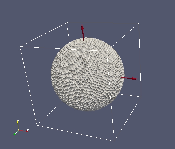
Figure 15: Visualization with ParaView of the dipole realization of a sphere, produced following above instructions, using files in directory examples_exp/ELLIPSOID.

32 Visualization of the Electric Field

The following instructions assume the user has the MayaVi2 graphics package installed. If you don’t have it yet, go to
http://code.enthought.com/projects/mayavi/mayavi/installation.html
for installation options.

1. First run example ELLIPSOID_NEARFIELD. This will produce output_1.vtr file.

2. Start Mayavi2

3. File/load data/open file output

4. Point to examples_exp/ELLIPSID_NEARFIELD/VTRoutput_1.vtr

5. colors and legends/add module/outline

6. outline/right click/add module/contour grid plane

7. In Mayavi2 object editor you can position slider between (0,95). Choose value in the middle. Set "filled contours" to on. Increase number of contours to 64.

8. One can add more "contour grid planes" to illustrate the results in different cross sections.

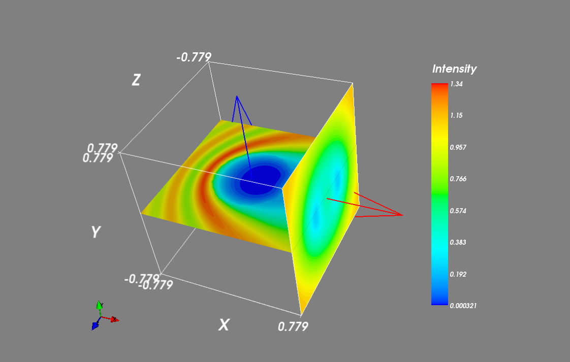
Figure 16: $|{\bf E}|/|{\bf E}_{0}|$ on two planes, one passing through the center and one passing near the $a=0.398{\mu{\rm m}}$ Au sphere calculated in examples_exp/ELLIPSOID_NEARFIELD. The incident wave, with $\lambda=0.5{\mu{\rm m}}$, is propagating with ${\bf k}_{0}\parallel\hat{\bf x}_{\rm TF}$. and ${\bf E}_{0}\parallel\hat{\bf y}_{\rm TF}$. The axes are labelled in ${\mu{\rm m}}$. This is the same problem as the results shown in Figure 14. This figure was generated by MayaVi2.

33 Finale

This User Guide is somewhat inelegant, but we hope that it will prove useful. The structure of the ddscat.par file is intended to be simple and suggestive so that, after reading the above notes once, the user may not have to refer to them again.

Known bugs in DDSCAT will be posted at the DDSCAT web site,
         http://code.google.com/p/ddscat/wiki/ReleaseNotes
and the latest version of DDSCAT can be found at
         http://code.google.com/p/ddscat/

Users are encouraged to provide B. T. Draine (draine@astro.princeton.edu) with their email address; email notification of bug fixes, and any new releases of DDSCAT, will be made known to those who do.

P. J. Flatau maintains the “SCATTERLIB - Light Scattering Codes Library" at
         http://code.google.com/p/scatterlib .
Emphasis is on providing source codes (mostly FORTRAN). However, other information related to scattering on spherical and non-spherical particles is collected: an extensive list of references to light scattering methods, refractive index, etc. This URL page contains section on the discrete dipole approximation.

Concrete suggestions for improving DDSCAT (and this User Guide) are welcomed.

Users of DDSCAT should cite appropriate papers describing DDA theory and its implementation. The following papers may be relevant (pdfs are included in the /doc directory)

• Draine (1988): basic theory of the DDA, including radiative reaction, and application to anisotropic materials;

• Goodman et al. (1990): introduction of FFT methods to greatly accelerate DDA calcualations

• Draine & Flatau (1994): review of the DDA, including demonstrations of accuracy and convergence;

• Draine & Flatau (2008): extension of the DDA to periodic structures, and generalization of the Mueller scattering matrix to describe scattering by 1-d and 2-d periodic structures.

• Flatau & Draine (2012): implementation of efficient near-field calculations using FFTs.

• This UserGuide.

34 Acknowledgments

• The routine ESELF making use of the FFT was originally written by Jeremy Goodman, Princeton University Observatory.

• The FFT routine FOURX, used in the comparison of different FFT routines, is based on a FFT routine written by Norman Brenner Brenner (1969).

• The GPFAPACK package was written by Clive Temperton (Temperton 1992), and generously made available by him for use with DDSCAT.

• Much of the work involved in modifying DDSCAT to use MPI was done by Matthew Collinge, Princeton University.

• The conjugate gradient routine ZBCG2 was written by M.A. Botchev
  (http://www.math.utwente.nl/$\sim$botchev/), based on earlier work by D.R. Fokkema (Dept. of Mathematics, Utrecht University).

• Art Lazanoff (NASA Ames Research Center) did most of the coding necessary to use OpenMP and to use the DFTI library routine from the Intel^® Math Kernel Library, as well as considerable testing of the new code.

• The conjugate gradient routine qpbicg.f90 was written by P.C. Chaumet and A. Rahmani (Chaumet & Rahmani 2009).

• The conjugate gradient routine qmrpim2.f90 is based on f77 code written by P.C. Chaumet and A. Rahmani.

• vtr.f90 was written by Jalel Chergui (LIMSI-CNRS).

• Ian Wong helped write subroutine BSELF and helped implement the filtered couple dipole option.

We are deeply indebted to all of these authors for making their work and code available.

We wish also to acknowledge bug reports and suggestions from DDSCAT users, including Rodrigo Alcaraz de la Osa, V. Choliy, Michel Devel, Souraya Goumri-Said, Bo Hu, Bala Krishna Juluri, Stefan Kniefl, Henrietta Lemke, Georges Levi, Shuzhou Li, Wang Lin, Paul Mulvaney, Timo Nousianen, Stuart Prescott, Honoh Suzuki, Sanaz Vahidinia, Bernhard Wasserman, Mike Wolff, and Hui Zhang.

Development of DDSCAT was supported in part by National Science Foundation grants AST-8341412, AST-8612013, AST-9017082, AST-9319283, AST-9616429, AST-9988126, AST-0406883, and AST-1008570 to BTD, in part by support from the Office of Naval Research Young Investigator Program to PJF, in part by DuPont Corporate Educational Assistance to PJF, and in part by the United Kingdom Defence Research Agency.

Appendix A Understanding and Modifying ddscat.par

In order to use DDSCAT to perform the specific calculations of interest to you, it will be necessary to modify the ddscat.par file. Here we list the sample ddscat.par file for the example problem in examples_exp/RCTGLPRSM, followed by a discussion of how to modify this file as needed. Note that all numerical input data in DDSCAT is read with free-format READ(IDEV,*)... statements. Therefore you do not need to worry about the precise format in which integer or floating point numbers are entered on a line. The crucial thing is that lines in ddscat.par containing numerical data have the correct number of data entries, with any informational comments appearing after the numerical data on a given line.

’ ========= Parameter file for v7.3 ===================’
’**** Preliminaries ****’
’NOTORQ’ = CMDTRQ*6 (NOTORQ, DOTORQ) -- either do or skip torque calculations
’PBCGS2’ = CMDSOL*6 (PBCGS2, PBCGST, GPBICG, PETRKP, QMRCCG) -- CCG method
’GPFAFT’ = CMDFFT*6 (GPFAFT, FFTMKL) -- FFT method
’GKDLDR’ = CALPHA*6 (GKDLDR, LATTDR, FLTRCD) -- DDA method
’NOTBIN’ = CBINFLAG (NOTBIN, ORIBIN, ALLBIN) -- specify binary output
’**** Initial Memory Allocation ****’
100 100 100 = dimensioning allowance for target generation
’**** Target Geometry and Composition ****’
’RCTGLPRSM’ = CSHAPE*9 shape directive
16 32 32  = shape parameters 1 - 3
1         = NCOMP = number of dielectric materials
’../diel/Au_evap’ = file with refractive index 1
’**** Additional Nearfield calculation? ****’
0 = NRFLD (=0 to skip nearfield calc., =1 to calculate nearfield E)
0.0 0.0 0.0 0.0 0.0 0.0 (fract. extens. of calc. vol. in -x,+x,-y,+y,-z,+z)
’**** Error Tolerance ****’
1.00e-5 = TOL = MAX ALLOWED (NORM OF |G>=AC|E>-ACA|X>)/(NORM OF AC|E>)
’**** maximum number of iterations allowed ****’
300     = MXITER
’**** Interaction cutoff parameter for PBC calculations ****’
1.00e-2 = GAMMA (1e-2 is normal, 3e-3 for greater accuracy)
’**** Angular resolution for calculation of <cos>, etc. ****’
0.5Ψ= ETASCA (number of angles is proportional to [(3+x)/ETASCA]^2 )
’**** Vacuum wavelengths (micron) ****’
0.5000 0.5000 1 ’LIN’ = wavelengths (first,last,how many,how=LIN,INV,LOG)
’**** Refractive index of ambient medium’
1.000 = NAMBIENT
’**** Effective Radii (micron) **** ’
0.246186 0.246186 1 ’LIN’ = aeff (first,last,how many,how=LIN,INV,LOG)
’**** Define Incident Polarizations ****’
(0,0) (1.,0.) (0.,0.) = Polarization state e01 (k along x axis)
2 = IORTH  (=1 to do only pol. state e01; =2 to also do orth. pol. state)
’**** Specify which output files to write ****’
1 = IWRKSC (=0 to suppress, =1 to write ".sca" file for each target orient.
’**** Prescribe Target Rotations ****’
0.    0.   1  = BETAMI, BETAMX, NBETA  (beta=rotation around a1)
0.    0.   1  = THETMI, THETMX, NTHETA (theta=angle between a1 and k)
0.    0.   1  = PHIMIN, PHIMAX, NPHI (phi=rotation angle of a1 around k)
’**** Specify first IWAV, IRAD, IORI (normally 0 0 0) ****’
0   0   0    = first IWAV, first IRAD, first IORI (0 0 0 to begin fresh)
’**** Select Elements of S_ij Matrix to Print ****’
6Ψ= NSMELTS = number of elements of S_ij to print (not more than 9)
11 12 21 22 31 41Ψ= indices ij of elements to print
’**** Specify Scattered Directions ****’
’LFRAME’ = CMDFRM (LFRAME, TFRAME for Lab Frame or Target Frame)
2 = NPLANES = number of scattering planes
0.   0. 180.  5 = phi, thetan_min, thetan_max, dtheta (in deg) for plane 1
90.  0. 180.  5 = phi, thetan_min, thetan_max, dtheta (in deg) for plane 2

Lines	Comments
1-2	comment lines
3	NOTORQ if torque calculation is not required;
	DOTORQ if torque calculation is required.
4	PBCGS2 is recommended; other options are PBCGST, GPBICG, PETRKP, and QMRCCG (see §12).
5	GPFAFT is supplied as default, but FFTMKL is recommended if DDSCAT has been compiled with
	the Intel® Math Kernel Library (see §§6.5, 13).
6	GKDLDR is recommended as the DDA method if the refractive index $m$ is not too large, but
	FLTRCD may be better if $|m|$ is large. (see §14)
7	NOTBIN for no unformatted binary output.
	ORIBIN for unformatted binary dump of orientational averages only;
	ALLBIN for full unformatted binary dump (§11.2);
8	comment line
9	initial memory allocation NX,NY,NZ. These must be large enough to accomodate the target that
	will be generated.
10	comment line
11	specify choice of target shape (see §21 for description of options RCTGLPRSM, ELLIPSOID,
	TETRAHDRN, …)
12	shape parameters SHPAR1, SHPAR2, SHPAR3, … (see §21).
13	number of different dielectric constant tables (see §15).
14	name(s) of dielectric constant table(s) (one per line).
15	comment line
16	NRFLD = 0, 1, 2 to skip, do nearfield calculation of ${\bf E}$, do nearfield calculation of both ${\bf E}$ and ${\bf B}$
17	6 non-negative numbers $r_{1},...,r_{6}$ specifying fractional extension of comptutational volume
	(in $-\hat{\bf x}_{\rm TF},+\hat{\bf x}_{\rm TF},-\hat{\bf y}_{\rm TF},+\hat{\bf y}_{\rm TF},-\hat{\bf z}_{\rm TF},+\hat{\bf z}_{\rm TF}$ direction (see §9.4)
18	commment line
20	TOL = error tolerance $h$: maximum allowed value of $|A^{\dagger}E-A^{\dagger}AP|/|A^{\dagger}E|$ [see eq.(19)].
21	comment line
22	MXITER$=$ maximum number of conjugate-gradient iterations allowed
23	comment line
24	GAMMA$=$ interaction cutoff parameter $\gamma$ (see Draine & Flatau 2009)
	the value of $\gamma$ does not affect calculations for isolated targets
25	comment line
26	ETASCA – parameter $\eta$ controlling angular averages (§25).
27	comment line
28	$\lambda$ – vacuum wavlenghts: first, last, how many, how chosen.
29	comment line
30	NAMBIENT$=$ (real) refractive index of ambient medium.
31	comment line
32	$a_{\rm eff}$ – first, last, how many, how chosen.
33	comment line
34	specify x,y,z components of (complex) incident polarization ${\hat{\bf e}}_{01}$ (§24)
35	IORTH = 2 to do both polarization states (normal);
	IORTH = 1 to do only one incident polarization.
36	comment line
37	IWRKSC = 0 to suppress writing of “.sca” files;
	IWRKSC = 1 to enable writing of “.sca” files.
38	comment line
39	$\beta$ (see §19) – first, last, how many .
40	$\Theta$ (see §19) – first, last, how many.
41	$\Phi$ (see §19) – first, last, how many.
42	comment line
43	IWAV0 IRAD0 IORI0 – starting values of integers IWAV IRAD IORI (normally 0 0 0).
44	comment line
45	$N_{S}$ = number of scattering matrix elements (must be $\leq 9$)
46	indices $ij$ of $N_{S}$ elements of the scattering matrix $S_{ij}$
47	comment line
48	specify whether scattered directions are to be specified by CMDFRM=’LFRAME’ or ’TFRAME’.
49	NPLANES$=$ number of scattering planes to follow
50	$\phi_{s}$ for first scattering plane, $\theta_{s,min}$, $\theta_{s,max}$, how many $\theta_{s}$ values;
51,…	$\phi_{s}$ for 2nd,… scattering plane, …

Appendix B wxxxryyy.avg Files

The file w000r000ori.avg contains the results for the first wavelength (w000) and first target radius (r000) averaged over orientations (.avg). The w000r000ori.avg file generated by the sample calculation in examples_exp/RCTGLPRSM should look like the following:

 DDSCAT --- DDSCAT 7.3.0 [12.12.29]
 TARGET --- Rectangular prism; NX,NY,NZ=  16  32  32
 GKDLDR --- DDA method
 PBCGS2 --- CCG method
 RCTGLPRSM --- shape
   16384     = NAT0 = number of dipoles
  0.06346821 = d/aeff for this target [d=dipole spacing]
    0.015625 = d (physical units)
  AEFF=      0.246186 = effective radius (physical units)
  WAVE=      0.500000 = wavelength (in vacuo, physical units)
K*AEFF=      3.093665 = 2*pi*aeff/lambda
NAMBIENT=    1.000000 = refractive index of ambient medium
n= ( 0.9656 ,  1.8628),  eps.= ( -2.5374 ,  3.5975)  |m|kd=  0.4120 for subs. 1
   TOL= 1.000E-05 = error tolerance for CCG method
( 1.00000  0.00000  0.00000 ) = target axis A1 in Target Frame
( 0.00000  1.00000  0.00000 ) = target axis A2 in Target Frame
  NAVG=   962 = (theta,phi) values used in comp. of Qsca,g
( 0.19635  0.00000  0.00000 ) = k vector (latt. units) in Lab Frame
( 0.00000, 0.00000 )( 1.00000, 0.00000 )( 0.00000, 0.00000 )=inc.pol.vec. 1 in LF
( 0.00000, 0.00000 )( 0.00000, 0.00000 )( 1.00000, 0.00000 )=inc.pol.vec. 2 in LF
   0.000   0.000 = beta_min, beta_max ;  NBETA = 1
   0.000   0.000 = theta_min, theta_max; NTHETA= 1
   0.000   0.000 = phi_min, phi_max   ;   NPHI = 1

 0.5000 = ETASCA = param. controlling # of scatt. dirs used to calculate <cos> etc.
 Results averaged over    1 target orientations
                   and    2 incident polarizations
          Qext       Qabs       Qsca      g(1)=<cos>  <cos^2>     Qbk       Qpha
 JO=1:  3.6134E+00  1.4308E+00  2.1827E+00  4.1463E-01 7.5169E-01 6.1831E-01 -1.2614E-01
 JO=2:  3.6135E+00 1.4308E+00 2.1827E+00  4.1463E-01 7.5169E-01 6.1831E-01 -1.2614E-01
 mean:  3.6134E+00  1.4308E+00  2.1827E+00  4.1463E-01 7.5169E-01 6.1831E-01 -1.2614E-01
 Qpol= -6.4373E-06                                                  dQpha= -4.9174E-07
         Qsca*g(1)   Qsca*g(2)   Qsca*g(3)   iter  mxiter  Nsca
 JO=1:  9.0502E-01 -3.2556E-09 -1.8964E-06     18    300    962
 JO=2:  9.0502E-01 -7.7139E-08  1.4648E-07     18    300    962
 mean:  9.0502E-01 -4.0197E-08 -8.7497E-07
            Mueller matrix elements for selected scattering directions in Lab Frame
 theta    phi    Pol.    S_11        S_12        S_21       S_22       S_31       S_41
  0.00   0.00  0.00000  7.5115E+01 -1.2970E-04 -1.297E-04  7.512E+01  6.785E-05 -2.220E-06
  5.00   0.00  0.00768  7.2167E+01 -5.5400E-01 -5.540E-01  7.217E+01  6.960E-05  6.113E-06
 10.00   0.00  0.03116  6.3968E+01 -1.9932E+00 -1.993E+00  6.397E+01  6.634E-05  1.229E-05
 15.00   0.00  0.07180  5.2244E+01 -3.7512E+00 -3.751E+00  5.224E+01  5.818E-05  1.351E-05
 20.00   0.00  0.13160  3.9245E+01 -5.1645E+00 -5.165E+00  3.924E+01  4.661E-05  1.559E-05
 25.00   0.00  0.21215  2.7088E+01 -5.7468E+00 -5.747E+00  2.709E+01  3.576E-05  1.251E-05
 30.00   0.00  0.31112  1.7234E+01 -5.3617E+00 -5.362E+00  1.723E+01  2.802E-05  9.135E-06
 35.00   0.00  0.41156  1.0271E+01 -4.2270E+00 -4.227E+00  1.027E+01  1.873E-05  6.317E-06
 40.00   0.00  0.46174  6.0117E+00 -2.7759E+00 -2.776E+00  6.012E+00  1.343E-05  1.892E-06
 45.00   0.00  0.38394  3.7970E+00 -1.4578E+00 -1.458E+00  3.797E+00  9.607E-06 -1.182E-06
 50.00   0.00  0.20310  2.8383E+00 -5.7645E-01 -5.765E-01  2.838E+00  7.253E-06 -1.685E-06
 55.00   0.00  0.08917  2.4759E+00 -2.2077E-01 -2.208E-01  2.476E+00  6.675E-06 -2.270E-06
 60.00   0.00  0.12808  2.2936E+00 -2.9377E-01 -2.938E-01  2.294E+00  6.400E-06 -1.932E-06
 65.00   0.00  0.28428  2.1074E+00 -5.9909E-01 -5.991E-01  2.107E+00  5.960E-06 -1.838E-06
 70.00   0.00  0.49621  1.8862E+00 -9.3596E-01 -9.360E-01  1.886E+00  5.212E-06 -1.174E-06
 75.00   0.00  0.70066  1.6630E+00 -1.1652E+00 -1.165E+00  1.663E+00  4.518E-06 -7.433E-07
 80.00   0.00  0.83815  1.4710E+00 -1.2329E+00 -1.233E+00  1.471E+00  3.404E-06 -2.239E-07
 85.00   0.00  0.87905  1.3178E+00 -1.1584E+00 -1.158E+00  1.318E+00  2.064E-06 -6.282E-07
 90.00   0.00  0.84390  1.1878E+00 -1.0024E+00 -1.002E+00  1.188E+00  1.096E-06 -6.092E-07
 95.00   0.00  0.78583  1.0596E+00 -8.3269E-01 -8.327E-01  1.060E+00  6.710E-07 -4.426E-07
100.00   0.00  0.75672  9.2363E-01 -6.9893E-01 -6.989E-01  9.236E-01  1.610E-07 -4.866E-08
105.00   0.00  0.78540  7.9128E-01 -6.2148E-01 -6.215E-01  7.913E-01  2.381E-07  2.968E-07
110.00   0.00  0.85741  6.9404E-01 -5.9507E-01 -5.951E-01  6.940E-01  8.433E-07  8.885E-07
115.00   0.00  0.89355  6.7418E-01 -6.0241E-01 -6.024E-01  6.742E-01  1.297E-06  1.225E-06
120.00   0.00  0.81395  7.7422E-01 -6.3018E-01 -6.302E-01  7.742E-01  1.748E-06  1.515E-06
125.00   0.00  0.65813  1.0320E+00 -6.7920E-01 -6.792E-01  1.032E+00  2.553E-06  1.802E-06
130.00   0.00  0.51335  1.4856E+00 -7.6264E-01 -7.626E-01  1.486E+00  3.536E-06  2.497E-06
135.00   0.00  0.40829  2.1850E+00 -8.9213E-01 -8.921E-01  2.185E+00  4.473E-06  3.066E-06
140.00   0.00  0.33090  3.2004E+00 -1.0590E+00 -1.059E+00  3.200E+00  6.583E-06  4.014E-06
145.00   0.00  0.26514  4.6139E+00 -1.2233E+00 -1.223E+00  4.614E+00  9.927E-06  4.933E-06
150.00   0.00  0.20350  6.4859E+00 -1.3199E+00 -1.320E+00  6.486E+00  1.326E-05  6.138E-06
155.00   0.00  0.14593  8.8035E+00 -1.2847E+00 -1.285E+00  8.804E+00  1.727E-05  7.720E-06
160.00   0.00  0.09522  1.1432E+01 -1.0886E+00 -1.089E+00  1.143E+01  1.989E-05  7.600E-06
165.00   0.00  0.05409  1.4098E+01 -7.6253E-01 -7.625E-01  1.410E+01  2.215E-05  7.833E-06
170.00   0.00  0.02413  1.6425E+01 -3.9641E-01 -3.964E-01  1.642E+01  2.194E-05  7.723E-06
175.00   0.00  0.00604  1.8022E+01 -1.0884E-01 -1.088E-01  1.802E+01  2.147E-05  6.818E-06
180.00   0.00  0.00000  1.8591E+01 -1.5259E-05 -1.526E-05  1.859E+01  1.746E-05  5.261E-06
  0.00  90.00  0.00000  7.5115E+01  1.2970E-04  1.297E-04  7.512E+01 -6.792E-05 -2.304E-06
  5.00  90.00  0.00767  7.2167E+01 -5.5382E-01 -5.538E-01  7.217E+01 -7.026E-05  1.632E-06
 10.00  90.00  0.03116  6.3968E+01 -1.9931E+00 -1.993E+00  6.397E+01 -6.760E-05  6.943E-06
 15.00  90.00  0.07180  5.2244E+01 -3.7513E+00 -3.751E+00  5.224E+01 -6.176E-05  1.252E-05
 20.00  90.00  0.13160  3.9245E+01 -5.1645E+00 -5.164E+00  3.924E+01 -5.102E-05  1.746E-05
 25.00  90.00  0.21216  2.7088E+01 -5.7468E+00 -5.747E+00  2.709E+01 -3.823E-05  2.014E-05
 30.00  90.00  0.31112  1.7234E+01 -5.3617E+00 -5.362E+00  1.723E+01 -2.451E-05  2.102E-05
 35.00  90.00  0.41156  1.0271E+01 -4.2270E+00 -4.227E+00  1.027E+01 -1.188E-05  1.911E-05
 40.00  90.00  0.46174  6.0117E+00 -2.7758E+00 -2.776E+00  6.012E+00 -1.197E-06  1.526E-05
 45.00  90.00  0.38394  3.7970E+00 -1.4578E+00 -1.458E+00  3.797E+00  6.698E-06  1.039E-05
 50.00  90.00  0.20309  2.8383E+00 -5.7643E-01 -5.764E-01  2.838E+00  1.136E-05  5.124E-06
 55.00  90.00  0.08916  2.4759E+00 -2.2076E-01 -2.208E-01  2.476E+00  1.306E-05  6.010E-07
 60.00  90.00  0.12807  2.2936E+00 -2.9375E-01 -2.937E-01  2.294E+00  1.260E-05 -2.887E-06
 65.00  90.00  0.28427  2.1074E+00 -5.9906E-01 -5.991E-01  2.107E+00  1.042E-05 -4.946E-06
 70.00  90.00  0.49620  1.8862E+00 -9.3594E-01 -9.359E-01  1.886E+00  7.425E-06 -5.874E-06
 75.00  90.00  0.70066  1.6630E+00 -1.1652E+00 -1.165E+00  1.663E+00  4.307E-06 -5.601E-06
 80.00  90.00  0.83814  1.4710E+00 -1.2329E+00 -1.233E+00  1.471E+00  1.319E-06 -4.684E-06
 85.00  90.00  0.87905  1.3178E+00 -1.1584E+00 -1.158E+00  1.318E+00 -1.179E-06 -3.851E-06
 90.00  90.00  0.84389  1.1878E+00 -1.0023E+00 -1.002E+00  1.188E+00 -2.932E-06 -2.944E-06
 95.00  90.00  0.78583  1.0596E+00 -8.3267E-01 -8.327E-01  1.060E+00 -3.904E-06 -2.553E-06
100.00  90.00  0.75672  9.2362E-01 -6.9892E-01 -6.989E-01  9.236E-01 -3.952E-06 -2.432E-06
105.00  90.00  0.78540  7.9127E-01 -6.2146E-01 -6.215E-01  7.913E-01 -3.187E-06 -2.802E-06
110.00  90.00  0.85741  6.9402E-01 -5.9506E-01 -5.951E-01  6.940E-01 -1.639E-06 -3.211E-06
115.00  90.00  0.89354  6.7417E-01 -6.0240E-01 -6.024E-01  6.742E-01  4.964E-07 -3.506E-06
120.00  90.00  0.81394  7.7422E-01 -6.3017E-01 -6.302E-01  7.742E-01  3.042E-06 -3.363E-06
125.00  90.00  0.65811  1.0320E+00 -6.7919E-01 -6.792E-01  1.032E+00  5.488E-06 -2.384E-06
130.00  90.00  0.51334  1.4856E+00 -7.6263E-01 -7.626E-01  1.486E+00  7.604E-06 -5.760E-07
135.00  90.00  0.40828  2.1850E+00 -8.9210E-01 -8.921E-01  2.185E+00  8.701E-06  1.924E-06
140.00  90.00  0.33089  3.2005E+00 -1.0590E+00 -1.059E+00  3.200E+00  8.507E-06  5.022E-06
145.00  90.00  0.26513  4.6139E+00 -1.2233E+00 -1.223E+00  4.614E+00  6.576E-06  8.175E-06
150.00  90.00  0.20349  6.4859E+00 -1.3198E+00 -1.320E+00  6.486E+00  3.323E-06  1.081E-05
155.00  90.00  0.14593  8.8035E+00 -1.2847E+00 -1.285E+00  8.804E+00 -1.197E-06  1.261E-05
160.00  90.00  0.09522  1.1432E+01 -1.0885E+00 -1.089E+00  1.143E+01 -6.047E-06  1.320E-05
165.00  90.00  0.05409  1.4098E+01 -7.6252E-01 -7.625E-01  1.410E+01 -1.070E-05  1.235E-05
170.00  90.00  0.02413  1.6425E+01 -3.9637E-01 -3.964E-01  1.642E+01 -1.452E-05  1.062E-05
175.00  90.00  0.00604  1.8022E+01 -1.0885E-01 -1.089E-01  1.802E+01 -1.681E-05  8.054E-06
180.00  90.00  0.00000  1.8591E+01  1.5259E-05  1.526E-05  1.859E+01 -1.742E-05  5.249E-06

Appendix C wxxxryyykzzz.sca Files

The w000r000k000.sca file contains the results for the first wavelength (w000), first target radius (r000), and first orientation (k000). The w000r000k000.sca file created by the sample calculation in examples_exp/RCTGLPRSM should look like the following:

 DDSCAT --- DDSCAT 7.3.0 [12.12.29]
 TARGET --- Rectangular prism; NX,NY,NZ=  16  32  32
 GKDLDR --- DDA method
 PBCGS2 --- CCG method
 RCTGLPRSM --- shape
   16384     = NAT0 = number of dipoles
  0.06346821 = d/aeff for this target [d=dipole spacing]
    0.015625 = d (physical units)
----- physical extent of target volume in Target Frame ------
     -0.250000      0.000000 = xmin,xmax (physical units)
     -0.250000      0.250000 = ymin,ymax (physical units)
     -0.250000      0.250000 = zmin,zmax (physical units)
  AEFF=      0.246186 = effective radius (physical units)
  WAVE=      0.500000 = wavelength (in vacuo, physical units)
K*AEFF=      3.093665 = 2*pi*aeff/lambda
NAMBIENT=    1.000000 = refractive index of ambient medium
n= ( 0.9656 ,  1.8628),  eps.= ( -2.5374 ,  3.5975)  |m|kd=  0.4120 for subs. 1
   TOL= 1.000E-05 = error tolerance for CCG method
( 1.00000  0.00000  0.00000 ) = target axis A1 in Target Frame
( 0.00000  1.00000  0.00000 ) = target axis A2 in Target Frame
  NAVG=   962 = (theta,phi) values used in comp. of Qsca,g
( 0.19635  0.00000  0.00000 ) = k vector (latt. units) in TF
( 0.00000, 0.00000 )( 1.00000, 0.00000 )( 0.00000, 0.00000 )=inc.pol.vec. 1 in TF
( 0.00000, 0.00000 )( 0.00000, 0.00000 )( 1.00000, 0.00000 )=inc.pol.vec. 2 in TF
( 1.00000  0.00000  0.00000 ) = target axis A1 in Lab Frame
( 0.00000  1.00000  0.00000 ) = target axis A2 in Lab Frame
( 0.19635  0.00000  0.00000 ) = k vector (latt. units) in Lab Frame
( 0.00000, 0.00000 )( 1.00000, 0.00000 )( 0.00000, 0.00000 )=inc.pol.vec. 1 in LF
( 0.00000, 0.00000 )( 0.00000, 0.00000 )( 1.00000, 0.00000 )=inc.pol.vec. 2 in LF
 BETA =  0.000 = rotation of target around A1
 THETA=  0.000 = angle between A1 and k
  PHI =  0.000 = rotation of A1 around k
 0.5000 = ETASCA = param. controlling # of scatt. dirs used to calculate <cos> etc.
          Qext       Qabs       Qsca      g(1)=<cos>  <cos^2>     Qbk       Qpha
 JO=1:  3.6134E+00  1.4308E+00  2.1827E+00  4.1463E-01 7.5169E-01 6.1831E-01 -1.2614E-01
 JO=2:  3.6135E+00  1.4308E+00  2.1827E+00  4.1463E-01 7.5169E-01 6.1831E-01 -1.2614E-01
 mean:  3.6134E+00  1.4308E+00  2.1827E+00  4.1463E-01 7.5169E-01 6.1831E-01 -1.2614E-01
 Qpol= -6.4373E-06                                                  dQpha= -4.9174E-07
         Qsca*g(1)   Qsca*g(2)   Qsca*g(3)   iter  mxiter  Nsca
 JO=1:  9.0502E-01 -3.2556E-09 -1.8964E-06     18    300    962
 JO=2:  9.0502E-01 -7.7139E-08  1.4648E-07     18    300    962
 mean:  9.0502E-01 -4.0197E-08 -8.7497E-07
            Mueller matrix elements for selected scattering directions in Lab Frame
 theta    phi    Pol.    S_11        S_12        S_21       S_22       S_31       S_41
  0.00   0.00  0.00000  7.5115E+01 -1.2970E-04 -1.297E-04  7.512E+01  6.785E-05 -2.220E-06
  5.00   0.00  0.00768  7.2167E+01 -5.5400E-01 -5.540E-01  7.217E+01  6.960E-05  6.113E-06
 10.00   0.00  0.03116  6.3968E+01 -1.9932E+00 -1.993E+00  6.397E+01  6.634E-05  1.229E-05
 15.00   0.00  0.07180  5.2244E+01 -3.7512E+00 -3.751E+00  5.224E+01  5.818E-05  1.351E-05
 20.00   0.00  0.13160  3.9245E+01 -5.1645E+00 -5.165E+00  3.924E+01  4.661E-05  1.559E-05
 25.00   0.00  0.21215  2.7088E+01 -5.7468E+00 -5.747E+00  2.709E+01  3.576E-05  1.251E-05
 30.00   0.00  0.31112  1.7234E+01 -5.3617E+00 -5.362E+00  1.723E+01  2.802E-05  9.135E-06
 35.00   0.00  0.41156  1.0271E+01 -4.2270E+00 -4.227E+00  1.027E+01  1.873E-05  6.317E-06
 40.00   0.00  0.46174  6.0117E+00 -2.7759E+00 -2.776E+00  6.012E+00  1.343E-05  1.892E-06
 45.00   0.00  0.38394  3.7970E+00 -1.4578E+00 -1.458E+00  3.797E+00  9.607E-06 -1.182E-06
 50.00   0.00  0.20310  2.8383E+00 -5.7645E-01 -5.765E-01  2.838E+00  7.253E-06 -1.685E-06
 55.00   0.00  0.08917  2.4759E+00 -2.2077E-01 -2.208E-01  2.476E+00  6.675E-06 -2.270E-06
 60.00   0.00  0.12808  2.2936E+00 -2.9377E-01 -2.938E-01  2.294E+00  6.400E-06 -1.932E-06
 65.00   0.00  0.28428  2.1074E+00 -5.9909E-01 -5.991E-01  2.107E+00  5.960E-06 -1.838E-06
 70.00   0.00  0.49621  1.8862E+00 -9.3596E-01 -9.360E-01  1.886E+00  5.212E-06 -1.174E-06
 75.00   0.00  0.70066  1.6630E+00 -1.1652E+00 -1.165E+00  1.663E+00  4.518E-06 -7.433E-07
 80.00   0.00  0.83815  1.4710E+00 -1.2329E+00 -1.233E+00  1.471E+00  3.404E-06 -2.239E-07
 85.00   0.00  0.87905  1.3178E+00 -1.1584E+00 -1.158E+00  1.318E+00  2.064E-06 -6.282E-07
 90.00   0.00  0.84390  1.1878E+00 -1.0024E+00 -1.002E+00  1.188E+00  1.096E-06 -6.092E-07
 95.00   0.00  0.78583  1.0596E+00 -8.3269E-01 -8.327E-01  1.060E+00  6.710E-07 -4.426E-07
100.00   0.00  0.75672  9.2363E-01 -6.9893E-01 -6.989E-01  9.236E-01  1.610E-07 -4.866E-08
105.00   0.00  0.78540  7.9128E-01 -6.2148E-01 -6.215E-01  7.913E-01  2.381E-07  2.968E-07
110.00   0.00  0.85741  6.9404E-01 -5.9507E-01 -5.951E-01  6.940E-01  8.433E-07  8.885E-07
115.00   0.00  0.89355  6.7418E-01 -6.0241E-01 -6.024E-01  6.742E-01  1.297E-06  1.225E-06
120.00   0.00  0.81395  7.7422E-01 -6.3018E-01 -6.302E-01  7.742E-01  1.748E-06  1.515E-06
125.00   0.00  0.65813  1.0320E+00 -6.7920E-01 -6.792E-01  1.032E+00  2.553E-06  1.802E-06
130.00   0.00  0.51335  1.4856E+00 -7.6264E-01 -7.626E-01  1.486E+00  3.536E-06  2.497E-06
135.00   0.00  0.40829  2.1850E+00 -8.9213E-01 -8.921E-01  2.185E+00  4.473E-06  3.066E-06
140.00   0.00  0.33090  3.2004E+00 -1.0590E+00 -1.059E+00  3.200E+00  6.583E-06  4.014E-06
145.00   0.00  0.26514  4.6139E+00 -1.2233E+00 -1.223E+00  4.614E+00  9.927E-06  4.933E-06
150.00   0.00  0.20350  6.4859E+00 -1.3199E+00 -1.320E+00  6.486E+00  1.326E-05  6.138E-06
155.00   0.00  0.14593  8.8035E+00 -1.2847E+00 -1.285E+00  8.804E+00  1.727E-05  7.720E-06
160.00   0.00  0.09522  1.1432E+01 -1.0886E+00 -1.089E+00  1.143E+01  1.989E-05  7.600E-06
165.00   0.00  0.05409  1.4098E+01 -7.6253E-01 -7.625E-01  1.410E+01  2.215E-05  7.833E-06
170.00   0.00  0.02413  1.6425E+01 -3.9641E-01 -3.964E-01  1.642E+01  2.194E-05  7.723E-06
175.00   0.00  0.00604  1.8022E+01 -1.0884E-01 -1.088E-01  1.802E+01  2.147E-05  6.818E-06
180.00   0.00  0.00000  1.8591E+01 -1.5259E-05 -1.526E-05  1.859E+01  1.746E-05  5.261E-06
  0.00  90.00  0.00000  7.5115E+01  1.2970E-04  1.297E-04  7.512E+01 -6.792E-05 -2.304E-06
  5.00  90.00  0.00767  7.2167E+01 -5.5382E-01 -5.538E-01  7.217E+01 -7.026E-05  1.632E-06
 10.00  90.00  0.03116  6.3968E+01 -1.9931E+00 -1.993E+00  6.397E+01 -6.760E-05  6.943E-06
 15.00  90.00  0.07180  5.2244E+01 -3.7513E+00 -3.751E+00  5.224E+01 -6.176E-05  1.252E-05
 20.00  90.00  0.13160  3.9245E+01 -5.1645E+00 -5.164E+00  3.924E+01 -5.102E-05  1.746E-05
 25.00  90.00  0.21216  2.7088E+01 -5.7468E+00 -5.747E+00  2.709E+01 -3.823E-05  2.014E-05
 30.00  90.00  0.31112  1.7234E+01 -5.3617E+00 -5.362E+00  1.723E+01 -2.451E-05  2.102E-05
 35.00  90.00  0.41156  1.0271E+01 -4.2270E+00 -4.227E+00  1.027E+01 -1.188E-05  1.911E-05
 40.00  90.00  0.46174  6.0117E+00 -2.7758E+00 -2.776E+00  6.012E+00 -1.197E-06  1.526E-05
 45.00  90.00  0.38394  3.7970E+00 -1.4578E+00 -1.458E+00  3.797E+00  6.698E-06  1.039E-05
 50.00  90.00  0.20309  2.8383E+00 -5.7643E-01 -5.764E-01  2.838E+00  1.136E-05  5.124E-06
 55.00  90.00  0.08916  2.4759E+00 -2.2076E-01 -2.208E-01  2.476E+00  1.306E-05  6.010E-07
 60.00  90.00  0.12807  2.2936E+00 -2.9375E-01 -2.937E-01  2.294E+00  1.260E-05 -2.887E-06
 65.00  90.00  0.28427  2.1074E+00 -5.9906E-01 -5.991E-01  2.107E+00  1.042E-05 -4.946E-06
 70.00  90.00  0.49620  1.8862E+00 -9.3594E-01 -9.359E-01  1.886E+00  7.425E-06 -5.874E-06
 75.00  90.00  0.70066  1.6630E+00 -1.1652E+00 -1.165E+00  1.663E+00  4.307E-06 -5.601E-06
 80.00  90.00  0.83814  1.4710E+00 -1.2329E+00 -1.233E+00  1.471E+00  1.319E-06 -4.684E-06
 85.00  90.00  0.87905  1.3178E+00 -1.1584E+00 -1.158E+00  1.318E+00 -1.179E-06 -3.851E-06
 90.00  90.00  0.84389  1.1878E+00 -1.0023E+00 -1.002E+00  1.188E+00 -2.932E-06 -2.944E-06
 95.00  90.00  0.78583  1.0596E+00 -8.3267E-01 -8.327E-01  1.060E+00 -3.904E-06 -2.553E-06
100.00  90.00  0.75672  9.2362E-01 -6.9892E-01 -6.989E-01  9.236E-01 -3.952E-06 -2.432E-06
105.00  90.00  0.78540  7.9127E-01 -6.2146E-01 -6.215E-01  7.913E-01 -3.187E-06 -2.802E-06
110.00  90.00  0.85741  6.9402E-01 -5.9506E-01 -5.951E-01  6.940E-01 -1.639E-06 -3.211E-06
115.00  90.00  0.89354  6.7417E-01 -6.0240E-01 -6.024E-01  6.742E-01  4.964E-07 -3.506E-06
120.00  90.00  0.81394  7.7422E-01 -6.3017E-01 -6.302E-01  7.742E-01  3.042E-06 -3.363E-06
125.00  90.00  0.65811  1.0320E+00 -6.7919E-01 -6.792E-01  1.032E+00  5.488E-06 -2.384E-06
130.00  90.00  0.51334  1.4856E+00 -7.6263E-01 -7.626E-01  1.486E+00  7.604E-06 -5.760E-07
135.00  90.00  0.40828  2.1850E+00 -8.9210E-01 -8.921E-01  2.185E+00  8.701E-06  1.924E-06
140.00  90.00  0.33089  3.2005E+00 -1.0590E+00 -1.059E+00  3.200E+00  8.507E-06  5.022E-06
145.00  90.00  0.26513  4.6139E+00 -1.2233E+00 -1.223E+00  4.614E+00  6.576E-06  8.175E-06
150.00  90.00  0.20349  6.4859E+00 -1.3198E+00 -1.320E+00  6.486E+00  3.323E-06  1.081E-05
155.00  90.00  0.14593  8.8035E+00 -1.2847E+00 -1.285E+00  8.804E+00 -1.197E-06  1.261E-05
160.00  90.00  0.09522  1.1432E+01 -1.0885E+00 -1.089E+00  1.143E+01 -6.047E-06  1.320E-05
165.00  90.00  0.05409  1.4098E+01 -7.6252E-01 -7.625E-01  1.410E+01 -1.070E-05  1.235E-05
170.00  90.00  0.02413  1.6425E+01 -3.9637E-01 -3.964E-01  1.642E+01 -1.452E-05  1.062E-05
175.00  90.00  0.00604  1.8022E+01 -1.0885E-01 -1.089E-01  1.802E+01 -1.681E-05  8.054E-06
180.00  90.00  0.00000  1.8591E+01  1.5259E-05  1.526E-05  1.859E+01 -1.742E-05  5.249E-06

Appendix D wxxxryyykzzz.poln Files

Binary files wxxxryyykzzz.poln are written to disk only when nearfield calculations are done (parameter NRFLD=1). The w000r000k000.pol1 file contains the polarization solution for the first wavelength (w000), first target radius (r000), first orientation (k000), and first incident polarization (pol1). In order to limit the size of this file, it has been written as an unformatted or "binary" file. This preserves full machine precision for the data, is quite compact, and can be read efficiently, but unfortunately the file is not fully portable because different computer architectures (e.g., Linux vs. MS Windows) have adopted different standards for storage of “unformatted” data. However, anticipating that many users will be computing within a single architecture, the distribution version of DDSCAT uses this format.

Additional warning: even on a single architecture, users should be alert to the possibility that different compilers may follow different conventions for reading/writing unformatted files.

The file contains the following information:

• The location of each dipole in the target frame.

• $(k_{x},k_{y},k_{z})d$, where $\bf k$ is the incident $k$ vector.

• $(E_{0x},E_{0y},E_{0z})$, the complex polarization vector of the incident wave.

• $\alpha^{-1}d^{3}$, the inverse of the symmmetric complex polarizability tensor for each of the dipoles in the target.

• $(P_{x},P_{y},P_{z})$, the complex polarization vector for each of the dipoles.

The interested user should consult the routine writepol.f to see how this information has been organized in the unformatted file.

Appendix E wxxxryyykzzz.En Files

Binary files wxxxryyykzzz.En are written to disk only when nearfield calculations of ${\bf E}$ (but not ${\bf B}$) are done (parameter NRFLD=1). The w000r000k000.E1 file contains information describing the problem and the solution at "grid points" throughout the extended "computational volume" specified for the nearfield calculation (see §29). These binary files are very large, but have been written in a way to simplify subsequent use for visualization using, e.g., the program DDPOSTPROCESS.f90 (see §32). The interested user can examine subroutine nearfield.f90 that writes the file, or program DDPOSTPROCESS.f90 that reads the file, to see how the information is organized.

A user who finds the file size to be a serious problem may wish to modify the code in nearfield.f90 to suppress writing of some of the arrays (e.g., the diagonal elements of the A matrix), retaining only the data of specific interest (e.g., the ${\bf E}$ field). Of course, and modifications to WRITE statements in nearfield.f90 will require corresponding changes to READ statements in subroutine readnf.f90 that DDPOSTPROCESS.f90 calls to read from the stored data files.

Appendix F wxxxryyykzzz.EBn Files

Binary files wxxxryyykzzz.EBn are written to disk only when nearfield calculations are done for both ${\bf E}$ and ${\bf B}$ (parameter NRFLD=2). The w000r000k000.EB1 file contains information describing the problem and the solution at "grid points" throughout the extended "computational volume" specified for the nearfield calculation (see §29). These binary files are very large, but have been written in a way to simplify subsequent use for visualization using, e.g., the program DDPOSTPROCESS.f90 (see §32). The interested user can examine subroutine nearfield.f90 that writes the file, or program DDPOSTPROCESS.f90 that reads the file, to see how the information is organized.

A user who finds the file size to be a serious problem may wish to modify the code in nearfield.f90 to suppress writing of some of the arrays (e.g., the diagonal elements of the A matrix), retaining only the data of specific interest (e.g., ${\bf B}_{{\rm sca}}$). Of course, and modifications to WRITE statements in nearfield.f90 will require corresponding changes to READ statements in DDPOSTPROCESS.f90.

References

- Bohren & Huffman (1983) Bohren, C. F. & Huffman, D. R., 1983. Absorption and Scattering of Light by Small Particles. New York: Wiley.
- Brenner (1969) Brenner, N. M., 1969. “Fast Fourier transform of externally stored data”. IEEE Trans. Audio and Electroacoustics, 17, 128–132.
- Chaumet & Rahmani (2009) Chaumet, P. C. & Rahmani, A., 2009. “Efficient iterative solution of the discrete dipole approximation for magnetodielectric scatterers”. Optics Letters, 34, 917–919.
- Collinge & Draine (2004) Collinge, M. J. & Draine, B. T., 2004. “Discrete dipole approximation with polarizabilities that account for both finite wavelength and target geometry”. J. Opt. Soc. Am., 21, 2023–2028.
- Draine (1988) Draine, B. T., 1988. “The Discrete-Dipole Approximation and its Application to Interstellar Graphite Grains”. Astrophys. J., 333, 848–872.
- Draine (2000) —, 2000. “The Discrete Dipole Approximation for Light Scattering by Irregular Targets”. In M. I. Mishchenko, J. W. Hovenier, & L. D. Travis, eds., “Light Scattering by Nonspherical Particles: Theory, Measurements, and Applications”, pp. 131–145. San Diego: Academic Press.
- Draine (2003) —, 2003. “Scattering by Interstellar Dust Grains. I. Optical and Ultraviolet”. Astrophys. J., 598, 1017–1025.
- Draine & Flatau (1994) Draine, B. T. & Flatau, P. J., 1994. “Discrete-dipole approximation for scattering calculations”. J. Opt. Soc. Am., 11, 1491–1499.
- Draine & Flatau (2008) —, 2008. “Discrete dipole approximation for periodic targets: I. Theory and tests”. J. Opt. Soc. Am., 25, 2693–2703.
- Draine & Goodman (1993) Draine, B. T. & Goodman, J., 1993. “Beyond Clausius-Mossotti - Wave Propagation on a Polarizable Point Lattice and the Discrete Dipole Approximation”. Astrophys. J., 405, 685–697.
- Draine & Weingartner (1996) Draine, B. T. & Weingartner, J. C., 1996. “Radiative Torques on Interstellar Grains. I. Superthermal Spin-up”. Astrophys. J., 470, 551–565.
- Flatau (1997) Flatau, P. J., 1997. “Improvements in the discrete-dipole approximation method of computing scattering and absorption”. Optics Letters, 22, 1205–1207.
- Flatau & Draine (2012) Flatau, P. J. & Draine, B. T., 2012. “Fast near-field calculations in the discrete dipole approximation for regular rectilinear grids”. Optics Express, 20, 1247–1252.
- Gay-Balmaz & Martin (2002) Gay-Balmaz, P. & Martin, O. J. F., 2002. “A library for computing the filtered and non-filtered 3D Green’s tensor associated with infinite homogeneous space and surfaces”. Comp. Phys. Comm., 144, 111–120.
- Goodman et al. (1990) Goodman, J. J., Draine, B. T., & Flatau, P. J., 1990. “Application of fast-Fourier transform techniques to the discrete dipole approximation”. Optics Letters, 16, 1198–1200.
- Gutkowicz-Krusin & Draine (2004) Gutkowicz-Krusin, D. & Draine, B. T., 2004. “Propagation of Electromagnetic Waves on a Rectangular Lattice of Polarizable Points”. ArXiv e-prints, http://arXiv.org/abs/astro-ph/0403082.
- Jackson (1975) Jackson, J. D., 1975. Classical electrodynamics, 2nd ed. New York: Wiley.
- Petravic & Kuo-Petravic (1979) Petravic, M. & Kuo-Petravic, G., 1979. “An ILUCG Algorithm Which Minimizes in the Euclidean Norm”. Journal of Computational Physics, 32, 263–269.
- Piller & Martin (1998) Piller, N. B. & Martin, O. J. F., 1998. “Increasing the performance of the coupled-dipole approximation: a spectral approach”. IEEE Transactions on Antennas and Propagation, 46, 1126–1137.
- Purcell & Pennypacker (1973) Purcell, E. M. & Pennypacker, C. R., 1973. “Scattering and Absorption of Light by Nonspherical Dielectric Grains”. Astrophys. J., 186, 705–714.
- Shen et al. (2008) Shen, Y., Draine, B. T., & Johnson, E. T., 2008. “Modeling Porous Dust Grains with Ballistic Aggregates I. Methods and Basic Results”. Astrophys. J., 689, 260–275.
- Sleijpen & Fokkema (1993) Sleijpen, G. L. G. & Fokkema, D. R., 1993. “BiCGSTAB(L) for linear matrices involving unsymmetric matrices with complex spectrum”. ETNA, 1, 11–32.
- Sleijpen & van der Vorst (1995) Sleijpen, G. L. G. & van der Vorst, H. A., 1995. “Maintaining convergence properties of BiCGstab methods in finite precision arithmetic”. Numerical Algorithms, 10, 203–223.
- Sleijpen & van der Vorst (1996) —, 1996. “Reliable updated residuals in hybrid Bi-CG methods”. Computing, 56, 141–163.
- Tang et al. (2004) Tang, J., Shen, Y., Zheng, Y., & Qiu, D., 2004. “An efficient and flexible computational model for solving the mild slope equation”. Coastal Engineering, 51, 143 – 154.
- Temperton (1992) Temperton, C., 1992. “A Generalized Prime Factor FFT Algorithm for any ”. SIAM J. Sci. Stat. Comput., 13, 676–686.
- Van der Vorst (1992) Van der Vorst, H. A., 1992. “BI-CGSTAB: A Fast and Smoothly Converging Variant of Bi-CG for the Solution of Nonsymmetric Linear Systems”. SIAM J. Sci. Stat. Comput., 13, 631–644.
- Yurkin et al. (2010) Yurkin, M. A., Min, M., & Hoekstra, A. G., 2010. “Application of the discrete dipole approximation to very large refractive indices: Filtered coupled dipoles revived”. Phys. Rev. E, 82, 036703.
- Zhang (1997) Zhang, S.-L., 1997. “GPBi-CG: Generalized Product-type Methods Based on Bi-CG for Solving Nonsymmetric Linear Systems”. SIAM Journal on Scientific Computing, 18, 537–551. URL http://link.aip.org/link/?SCE/18/537/1.