Social Sensor Placement in Large Scale Networks: A Graph Sampling Perspective

Abstract

Sensor placement for the purpose of detecting/tracking news outbreak and preventing rumor spreading is a challenging problem in a large scale online social network (OSN). This problem is a kind of subset selection problem: choosing a small set of items from a large population so to maximize some prespecified set function. However, it is known to be NP-complete. Existing heuristics are very costly especially for modern OSNs which usually contain hundreds of millions of users. This paper aims to design methods to find good solutions that can well trade off efficiency and accuracy. We first show that it is possible to obtain a high quality solution with a probabilistic guarantee from a “candidate set” of the underlying social network. By exploring this candidate set, one can increase the efficiency of placing social sensors. We also present how this candidate set can be obtained using “graph sampling”, which has an advantage over previous methods of not requiring the prior knowledge of the complete network topology. Experiments carried out on two real datasets demonstrate not only the accuracy and efficiency of our approach, but aslo effectiveness in detecting and predicting news outbreak.

I. Introduction

The rising popularity of online social networks (OSNs) has made information sharing and discovery much easier than ever before. Such social networks shift the role of participants from few content producers with many consumers to both producers and consumers of content. While this fundamental change enables information diversity in the Internet, it introduces the problem of what information sources to subscribe to or follow due to users’ limited attention capacities. For example, journalists need to discover breaking news from OSNs in a timely manner, while government officers may want to prevent damages caused by destructive riots arose from OSNs (e.g., the England Riots in 2011), or twitter users may want to track valuable information by following limited twitter accounts. Hence, it is important to decide which subset of social network accounts to choose as information sources such that the total information obtained is maximized.

The task of selecting a small number of accounts (or nodes) to cover as much valuable information as possible is feasible in modern OSNs because messages are shared by users, e.g., a tweet related to breaking news can be retweeted, reposted or shared by the followers or friends in social networks. Therefore, one only needs to read one participant’s tweets and obtain the information about the event. Here, we say that diffusible tweets triggered by some users and the associated participants form many information cascades, and the social network accounts which we prefer to select to monitor are called social sensors. Our problem is how to select a finite number of social sensors which can discover as many important cascades as possible.

Challenges: Selecting a small set of items from a large population to maximize some prespecified set function is a classical combinatorial optimization problem and its solution has widespread application, e.g, set cover problem(?; ?), influence maximization(?; ?) and optimal sensing(?; ?). However, all these works assume that the complete data (i.e., network topology) is available in advance. For modern OSNs, the network topology is usually not available. This is because many of these OSNs have hundreds of millions of accounts, and OSN service providers usually limit the request rates. This makes the task of discovering the entire network topology very difficult, if not impossible. Secondly, even if we know the network topology, the underlying subset selection problem is NP-complete. When the objective function is submodular, a greedy algorithm (GA) can find a solution with the lower bound of $1-1/e\approx 63\%$ to the optimal solution(?), and its execution time is polynomial to the size of network. However, the algorithm does not scale to handle large graphs like modern OSNs since they usually have hundreds of millions of nodes. The current state-of-the-art approach is the Accelerated Greedy (AG)(?). However, it is not guaranteed to be efficient all the time, i.e., in the worst case, it is as inefficient as the greedy algorithm. Thirdly and most importantly, the purpose of placing social sensors is to capture “future” important events, i.e., sensors selected based on historical data should have good predictive capability of future information cascades. However, users in OSNs are highly dynamic, e.g., everyday many new users join in and many existing users drop out. This will lead to a poor predictive capability of sensors selected based solely on old historical data. To improve sensors’ predictive capability, one has to periodically reselect sensors. Therefore, we need a computationally efficient social sensor placement algorithm that can accurately capture important future events.

Proposed Approach: The above challenges inspire us to develop computationally efficient, cheaper (no need to have the topology of an OSN beforehand) methods that provide quality guarantees. In this paper, we introduce an approach based on graph sampling(?; ?). The basic idea is that by carefully choosing a set of candidate sensors, we can select the final sensors from this candidate set. By sampling, the search space can be reduced dramatically and efficiency is increased. In this study, we show that graph sampling can be used to find solutions with probabilistic quality guarantees.

Results: We conduct experiments on two real datasets Sina Weibo and Twitter, which are the two most popular microblogs in the world, and compare our results with existing state-of-the-art methods. We not only demonstrate our approach is computationally efficient, but we also show that random walk based sampling can produce higher quality candidate sets than vertex sampling. Finally, we apply our method to Sina Weibo and show the effectiveness of sensors’ detection and prediction capability on discovering events.

This paper is organized as follows. In Section II, we introduce notations and formulate the problem. The basic framework of the proposed method is introduced in Section III along with performance guarantee analysis. Experiments are conducted in Section IV. Section V summarizes the related works, and Section VI concludes.

II. Problem Statement

Let us first introduce some notations we use in this paper, and then formally present the problem formulation.

Notations and Problem Formulation

Let $G(V,E,C)$ denote the OSN under study, where $V$ is the set of nodes, $E$ is the set of edges, and $C$ is the set of information cascades. An information cascade (or cascade for short) $c\in C$ is represented by a set of participating times $\{t_{cu}:u\in V,c\in C,t_{cu}\geq 0\}$, where $t_{cu}$ denotes the time that node $u$ first participates cascade $c$. If $u$ never joins $c$ during our observation then $t_{cu}=\infty$. The size of a cascade is the number of users with a finite participating time, denoted by $size(c)$, i.e., $size(c)=|\{u:u\in V\wedge t_{cu}<\infty\}|$. Also, let $t_{c}$ denote the time cascade $c$ begins, i.e., $t_{c}=\min_{u}t_{cu}$. A summary of these notations is shown in Table 1.

Table 1: Frequently used notations.

Notation	Description
$G(V,E,C)$	Social network, $V$, $E$ and $C$ are node/edge/cascade sets.
$t_{cu}$	The time user $u$ participates cascade $c$.
$t_{c}$	The start time of cascade $c$, $t_{c}=\min_{u}t_{cu}$.
$Nb(u)$	Neighboring nodes of node $u$.
$B,B^{\prime}$	Budget of finding sensors and candidates respectively.
$K$	Greedy algorithm stops after $K$ rounds, where $K\leq B$.
$F(\cdot)$	Reward function we want to optimize.
${\cal C},{\cal C}_{k}$	Set of candidates or candidates at round $k$.
$S,S_{k}$	Set of sensors or sensors obtained after round $k$.
$S_{\alpha}^{*}$	Top $\alpha\%$ of the nodes ordered by reward gain decreasingly.
$OPT$	The optimal solution of problem (1).
$\delta_{s}(S)$	Reward gain of node $s$ with respect to $S$.
$\xi_{p}(\alpha)$	Sample size with confidence $p$ and percentile $\alpha$.

The social sensor placement problem is to select a set of nodes $S\subset V$ as social sensors within budget $B$, where $|S|\leq B\ll|V|$, so as to maximize a reward function $F(S)$, which is a set function $F:2^{V}\rightarrow\mathbb{R}_{\geq 0}$ and satisfies $F(\emptyset)=0$. The optimal sensor set $OPT$ satisfies

$$OPT=\mathop{\arg\max}_{S\subset V\wedge|S|\leq B}F(S).$$ (1)

The reward function, in general, is determined by requirements of the problem under study(?). In this paper, we want to trade off importance (quantified by $size(c)$) against timeliness (quantified by $t_{cu}-t_{c}$), which results in the following,

$$F(S)=\sum_{c\in C}\frac{size(c)}{1+\min_{u\in S}\{t_{cu}-t_{c}\}}.$$ (2)

That is, if the sensor set $S$ can cover as many large size cascades as early as possible, the reward will be high.

Submodularity and Greedy Algorithm

Optimization problem (1) is NP-complete(?). However, when $F$ is a) nondecreasing, i.e., if $S\subseteq T\subseteq V$, then $F(S)\leq F(T)$, and b) submodular, i.e., if $S\subseteq T\subseteq V$, then $F(S\cup\{s\})-F(S)\geq F(T\cup\{s\})-F(T)$, $\forall s\in V\backslash T$, the greedy algorithm can obtain an approximate solution that is at least $1-1/e\approx 63\%$ of the optimal(?). It is easy to show that Eq. (2) possesses these two properties.

The greedy algorithm can be stated as follows. It runs for at most $B$ rounds to obtain a set $S$ of size $|S|\leq B$. In each round, it finds a node $s\in V\backslash S$ that maximizes the reward gain $\delta_{s}(S)\triangleq F(S\cup\{s\})-F(S)$, then $s$ is added into $S$ in this round. This process repeats $K$ rounds until $|S|=B$ or $\delta_{s}(S)=0$. The computation complexity of this algorithm is $O(K\cdot|V|)$. Note that this greedy algorithm is not scalable for large scale OSNs since graphs of these OSNs usually have large number of nodes (or $|V|$ is very large).

To speed up the greedy algorithm, Leskovec et al(?) use a Cost-Effective Lazy Forward (CELF) approach, also known as Accelerated Greedy (AG) proposed in (?) to reduce the computation times of $\delta_{s}(S)$ in each round by further utilizing the submodularity of $F$. The basic idea is that the reward gain of a node in the current round cannot be better than its reward gain in the previous round, i.e., if $k>l$, then $\delta_{s}(S_{k})\leq\delta_{s}(S_{l}),\,\forall s\in V\backslash S_{k}$, where $S_{k},1\leq k\leq K$ is the selected nodes after the $k$-th round by the greedy algorithm. However, it is important to note that AG/CELF does not guarantee an improvement on computational efficiency, i.e., in the worst case, it is as inefficient as the naive greedy algorithm(?).

III. Search Space Reduction

The inefficiency of the above mentioned algorithms is due to the large search space and the absence of an efficient search method. For example, to find at most $B$ sensors from the node set $V$, there are $\sum_{n=1}^{B}\binom{|V|}{n}=O(2^{|V|})$ possible solutions. Hence, we modify our problem, and consider how to find some acceptable good solutions at a much lower computational cost. In the following, we first describe the basic framework of our approach and present the definition of acceptable good solution of our algorithm. We then formally show the performance guarantees of the proposed approach, along with its variants and cost analysis.

The Basic Framework

In order to reduce search space, we consider using a candidate set ${\cal C}_{k}\!\subseteq\!V\backslash S_{k-1}$ to represent the search space at round $k$. This forms the basic search space reduction framework as described in Alg. 1 (We sometimes suppress the subscript $k$ if there is no ambiguity).

Input: Nodes $V$, budget $B$.

Output: Sensors $S$.

1 $S=\emptyset$;

2 while $|S|<B$, do

3       Generate candidate set ${\cal C}\subseteq V\backslash S$;

4       Select a node $\hat{s}^{*}$ such that $\hat{s}^{*}=\mathop{\arg\max}_{s\in{\cal C}}\delta_{s}(S)$;

5       $S=S\cup\{\hat{s}^{*}\}$;

6      

7 end while

Algorithm 1 The basic framework

The only difference between Alg. 1 and the original greedy algorithm is the process at line 1. In the original algorithm, one selects a node $s^{*}$ from $V\backslash S$ that maximizes the reward gain $\delta_{s}(S)$. Here, we select $\hat{s}^{*}$ from a candidate set ${\cal C}\subseteq V\backslash S$ to maximize $\delta_{s}(S)$. Intuitively, the accuracy of this algorithm should be arbitrary close to the greedy algorithm as ${\cal C}\rightarrow V\backslash S$ at each round but with a reduction in computational cost. Furthermore, if the sample size at each round is the same, then Alg. 1 becomes $|V|/|{\cal C}|$ times faster than the original greedy algorithm. In later sub-section, we will present algorithms on how to generate the candidate set ${\cal C}$. Let us first define what we mean by acceptable good solutions.

Acceptable Good Solutions

At round $k$, suppose we rank the nodes in $V\backslash S_{k-1}$ by reward gain in a decreasing order, and denote the top $\alpha\%$ of the nodes by $S_{\alpha}^{*}$, where $\alpha\in(0,100]$. If $\hat{s}^{*}$ falls into $S_{\alpha}^{*}$, we say $\hat{s}^{*}$ is an acceptable good sensor found in round $k$. It is obvious that one needs to set $\alpha$ to be small, say less than 1, so to find acceptable good sensors. All acceptable good sensors found after $K$ rounds form the acceptable good solution of Alg. 1.

The candidate set size $|{\cal C}|$ will affect the likelihood that at least one node in ${\cal C}$ falls into $S_{\alpha}^{*}$. Formally, we can calculate the probability that at least $k$ nodes in ${\cal C}$ falls into $S_{\alpha}^{*}$ as

$$Prob\{|{\cal C}\cap S_{\alpha}^{*}|\geq k\}=\sum_{i=k}^{|S_{\alpha}^{*}|}\frac{\binom{|S_{\alpha}^{*}|}{i}\binom{|V\backslash S_{\alpha}^{*}|}{|{\cal C}|-i}}{\binom{|V|}{|{\cal C}|}},$$ (3)

which follows a hypergeometric distribution. For $k=1$, this is equivalent to

$$Prob\{|{\cal C}\cap S_{\alpha}^{*}|\geq 1\}=1-(1-\alpha\%)^{|{\cal C}|}.$$ (4)

In order to achieve a confidence level that $Prob\{|{\cal C}\cap S_{\alpha}^{*}|\geq 1\}\geq p$, we can determine the lower bound on $|{\cal C}|$ as

$$|{\cal C}|\geq\left\lceil\frac{\ln(1-p)}{\ln(1-\alpha\%)}\right\rceil.$$ (5)

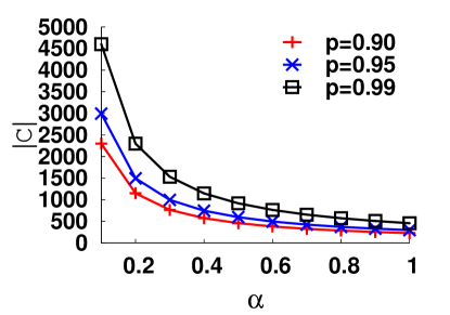
(a) Candidates size $|{\cal C}|$.

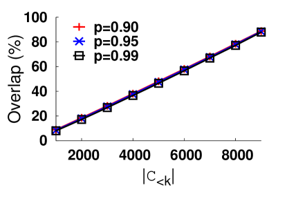
(b) Overlap percentile.

Figure 1: (a) Reduction of $|{\cal C}|$ as we increase $\alpha$. (b) For a small network of $|V|=10000$ and $|{\cal C}_{k}|=1000$ nodes, there is a high degree of overlap.

Fig. 1a shows the relationship between $|{\cal C}|$ and $\alpha$ with three different confidence levels of $p$, which we set to 0.90, 0.95 and 0.99. One interesting observation is that, when $\alpha$ varies from 0.1 to 1 (or top 0.1% to 1%), $|{\cal C}|$ drops quickly, which means that the search space size can be dramatically reduced. For example, if we want to choose a node in top 1% (or $\alpha\!=\!1$) of the best nodes from the whole population, then one can be sure that one of the 458 nodes will be a good sensor with probability greater than 0.99. There is one technical issue we need to pay attention:

Dealing with small networks. When the network is small, the advantage of using our framework is not significant. We can further improve the efficiency of Alg. 1 by exploiting the submodular property of reward functions as used in (?; ?). One conclusion from Eq. (3) is that, when $|V|$ is small, at round $k$, the overlap between previous candidates ${\cal C}_{<k}=\bigcup_{i=1}^{k-1}{\cal C}_{i}$ and current candidates ${\cal C}_{k}$, i.e., $|{\cal C}_{<k}\cap{\cal C}_{k}|$, is large and increases as $|{\cal C}_{<k}|$ increasing. An example is illustrated in Fig. 1b. In the example, we have a small network and its size is set to $|V|=10000$. At each round, $1000$ candidates are selected. We show the least overlap percentile versus selected candidate set size $|{\cal C}_{<k}|$ with a given confidence $p$. For example, when $1000$ candidates have been selected in the previous rounds, for a newly $1000$ selected candidates, there is a guarantee that at least 8% of them have been selected in previous rounds with probability greater than 0.99. For those overlapped nodes, we can reduce the calculations of updating reward gain by utilizing the submodular property. This will reduce the computational complexity of our framework.

To achieve this, we can store the candidate node $u$ and its reward gain $\delta_{u}$ in a tuple $\langle u,\delta_{u},\#_{u}\rangle$. Here $\#_{u}$ is the round during which the reward gain of node $u$ is calculated or updated. For candidates ${\cal C}_{k}$, we only need to calculate the reward gain of newly selected nodes and we do not need to update the reward gain of previously selected nodes immediately. We arrange nodes in ${\cal C}_{k}$ as a priority queue $Q$ by descending order of reward gain. Then we access the head $v$ of $Q$ to check whether $\#_{v}$ equals to the current round $k$. If yes, then $v$ is added into $S$; otherwise, update $v$’s reward gain, and put $v$ into $Q$ again. This way, the times of updating reward gain of sampled nodes can be reduced and Alg. 1 will be at least as efficient as AG/CELF when dealing with small networks.

Performance Analysis

We conclude from our previous discussion that we can probabilistically guarantee in selecting an acceptable sensor at each round from a small candidate set ${\cal C}$. Here, we quantify the quality of the final sensor set obtained after $K$ rounds. That is, how close the solution obtained by Alg. 1 is to the optimal solution of problem (1)? The following theorem answers this question.

Theorem 1.

Denote the set of sensors obtained by Alg. 1 after round $k$ as $S_{k}=\{\hat{s}_{1}^{*},\cdots,\hat{s}_{k}^{*}\}$, $1\leq k\leq K$. Let $\lambda_{k}=\delta_{\hat{s}_{k}^{*}}(S_{k-1})/\delta_{s_{k}^{*}}(S_{k-1})\in(0,1]$, where $s_{k}^{*}=\mathop{\arg\max}_{s\in V\backslash S_{k-1}}\delta_{s}(S_{k-1})$. Let $\lambda=\min_{1\leq k\leq K}\lambda_{k}$, then

$$F(S_{K})\geq(1-\frac{1}{e^{\lambda}})F(OPT).$$ (6)

Proof: Please refer to the Appendix.  

Remark: Theorem 1 indicates an important property of Alg. 1, i.e., if at each step the reward gain $\delta_{\hat{s}^{*}}(S)$ is bounded by a factor $\lambda$, then the final solution is bounded by another factor $1-1/e^{\lambda}$. When $\lambda\approx 1$, our final solution is $1\!-\!1/e\approx 63\%$ of the $OPT$. Hence, Alg. 1 guarantees a good solution when $\lambda$ is close to one. Note that in general, one cannot guarantee that $\lambda$ is close to one all the time. For example, the reward gain of the second best node is much less than the best node in current round. In such a case, finding the best node is like finding a needle in a haystack, which illustrates the intrinsic difficulty due to the reward distribution. Nevertheless, one can still accept the approximate solution if we believe the second best solution has a reward which is not significantly different from the best solution.

One can also understand the quality of Alg. 1 from another point of view. We define cover ratio as the fraction of nodes in $OPT$ that are in all candidate sets, i.e., $r=|\bigcup_{k=1}^{K}{\cal C}_{k}\cap OPT|/K$. Intuitively, the higher the cover ratio, the better the quality of the final solution. Assume the size of candidate set equal in each round, and denote it by $\xi_{p}(\alpha)$ with confidence $p$ and percentile $\alpha$. The following theorem presents a lower bound on the expectation of cover ratio for fixed $p$ and $\alpha$.

Theorem 2.

If we set $\alpha=100K/|V|$ at each round, then $\mathbb{E}[r]\geq 1-1/e^{p}$.

Proof: Please refer to the Appendix.  

Remark: Because $p$ can be very close to 1, $1-1/e^{p}$ will be very close to $1-1/e\approx 0.63$. In fact, the cover ratio can be further improved by increasing sample size at each round, e.g., we can derive in a similar manner that if we set $\alpha=50K/|V|$, then the expected cover ratio will be at least 0.82, or 82% of those sensors in $OPT$.

Generating ${\cal C}$ via Graph Sampling Methods

In previous discussion, we did not specify precisely how to generate the candidate set ${\cal C}$. In fact, ${\cal C}$ can be generated by randomly selecting nodes in $V$. This does not exploit any structural properties of OSNs, hence the performance discussed in previous sub-section can be viewed as the worst case guarantee. Here, we show how to use graph sampling to generate ${\cal C}$. The main advantage of using graph sampling is that one does not need to know the complete graph topology prior to executing the sensor placement algorithm. This is one main advantage of our framework as compare with the current state-of-the-art approaches(?; ?). Furthermore, we also want to explore how different graph sampling methods may affect sensor quality. Hence, we make two modification to Alg. 1:

• Instead of selecting new candidates in each round, we construct one candidate set ${\cal C}$ at the beginning of the algorithm;

• When a node $v$ is sampled, we select a candidate node, say $s$, from $v$ or one of $v$’s neighbors (i.e., $\{v\}\cup Nb(v)$) which can maximize the reward gain and we put $s$ into ${\cal C}$.

The second change is useful in filtering out noisy tweets in OSNs (e.g., tweets containing unimportant cascades), and reduces the candidate set size. Nodes with large reward gain in the neighborhood are more preferred to be in ${\cal C}$.

Vertex sampling (VS) and random walk (RW) are two popular graph sampling methods. We design two variants of Alg. 1 based on vertex sampling and random walk respectively, they are illustrated in Algs. 2 and 3.

Input: Network $G$, sensor budget $B$, candidate budget $B^{\prime}$.

Output: Sensors $S$.

1 ${\cal C}=\emptyset$;

2 while $|{\cal C}|<B^{\prime}$, do

3       Choose a node $v\in V\backslash{\cal C}$;

4       Select a node $s^{*}$ such that $s^{*}=\mathop{\arg\max}_{s\in Nb(v)\cup\{v\}}\delta_{s}({\cal C})$;

5       ${\cal C}={\cal C}\cup\{s^{*}\}$;

6      

7 end while

$S=Greedy({\cal C},B)$ ;

  /* choose $B$ sensors from ${\cal C}$ using the greedy algorithm */

Algorithm 2 Combining with vertex sampling

Input: Network $G$, sensor budget $B$, candidate budget $B^{\prime}$.

Output: Sensors $S$.

1 ${\cal C}=\emptyset$;

2 Set $u=u_{0}$ which is randomly chosen from $V$;

3 while $|{\cal C}|<B^{\prime}$, do

4       Choose a node $v\in Nb(u)$;

5       Select the node $s^{*}$ such that $s^{*}=\mathop{\arg\max}_{s\in Nb(v)}\delta_{s}({\cal C})$;

6       ${\cal C}={\cal C}\cup\{s^{*}\}$;

7       Set $u=v$;

8      

9 end while

$S=Greedy({\cal C},B)$ ;

  /* choose $B$ sensors from ${\cal C}$ using the greedy algorithm */

Algorithm 3 Combining with random walk

Each of these algorithms contains two steps. In the first step, the candidate set ${\cal C}$ with budget $B^{\prime}$ are constructed. In the second step, the final sensors $S$ are chosen. In line 2 of Alg. 2 and line 3 of Alg. 3, we can use various attribute information within an OSN to bias the selection. Such attributes of a user can be the number of posts/friends/followers and so on. For example, when using random walk to build the candidate set (Alg. 3), we can choose a neighboring node with probability proportion to its degree or activity (#posts), which will bias a random walk toward high degree or activity nodes. Intuitively, large degree nodes are more likely to be information sources or information hubs, and high activity nodes are more likely to retweet tweets. The comparison of using different attributes to bias our node selection will be discussed in Section IV. Although vertex sampling cannot be biased without knowing attributes of every node in advance, in order to study functions of different attributes, we will assume we know this complete information and let vertex sampling be biased by different attributes.

Sampling Cost Analysis

The computational cost of social sensor selection is defined to be the number of times that the reward gain of nodes is calculated or updated. Because of the second change in Alg. 2 and Alg. 3, there will be additional cost in obtaining samples ${\cal C}$. Here, we analyze the cost of sampling using uniform vertex sampling (UVS) (for Alg. 2) and uniform random walk (URW) (for Alg. 3).

For UVS in Alg. 2, the average cost to obtain candidate set ${\cal C}$ is

$$Cost_{\text{UVS}}=\mathbb{E}[\sum_{i=1}^{B^{\prime}}(d_{i}+1)]=B^{\prime}(1+\mathbb{E}[d_{\text{UVS}}]),$$

where $d_{i}$ is the degree of $i$-th node in ${\cal C}$, and $\mathbb{E}[d_{\text{UVS}}]$ is the average node degree obtained by UVS. Let $M$ denote the maximum degree in the network, and $\theta_{d}$ the fraction of nodes with degree $d$. Then $\mathbb{E}[d_{\text{UVS}}]=\sum_{d=1}^{M}d\theta_{d}\triangleq d_{\text{avg}}$. For power law networks with degree distribution $\theta_{d}=\frac{1}{Z}d^{-a}$, we obtain

$$\mathbb{E}[d_{\text{UVS}}]=\frac{1}{Z}\sum_{d=1}^{M}d^{1-a}.$$ (7)

For URW, the average cost to obtain candidate set ${\cal C}$ can be derived similarly, that is

$$Cost_{\text{URW}}=\mathbb{E}[\sum_{i=1}^{B^{\prime}}d_{i}]=B^{\prime}\cdot\mathbb{E}[d_{\text{URW}}],$$

where $\mathbb{E}[d_{\text{URW}}]$ is the average node degree under URW, i.e., $\mathbb{E}[d_{\text{URW}}]=\sum_{d=1}^{M}d\frac{d\theta_{d}}{d_{\text{avg}}}$. For power law networks, it becomes

$$\mathbb{E}[d_{\text{URW}}]=\frac{1}{Zd_{\text{avg}}}\sum_{d=1}^{M}d^{2-a}.$$ (8)

Equations (7) and (8) reveal the difference between UVS and URW. Both of them are functions of $a$, the exponent of the power law degree distribution. The difference is that, for UVS, $\mathbb{E}[d_{\text{UVS}}]$ is always finite when $a>2$, which means that the average cost of obtaining a sample equal the average degree, and it is usually small and bounded by the Dunbar number. For URW, $\mathbb{E}[d_{\text{URW}}]$ is finite if $a>3$; otherwise the average cost can become arbitrarily large as $M$ increases.

To limit the cost of creating candidate set, we can use simple heuristics to avoid searching a local maximum reward gain node from all the neighbors. For example, we can limit the searching scope to the top $n$ most active neighbors. In our experiments, $n$ can be set very small (e.g., 10), so the cost of obtaining samples will be bounded by $O(B^{\prime}\cdot n)$.

IV. Experiments

To evaluate the performance of previous discussed methods, we present experimental results on two datasets collected from Sina Weibo and Twitter, respectively. Then, we conduct experiments on Sina Weibo to study the detection capability, which measures the ability to detect cascades, as well as prediction capability, which measures the ability to capture future cascades using the senors selected based on historial data.

Table 2: Dataset summary

Dataset	Sina Weibo	Twitter
Nodes	0.3M	1.7M
Edges	1.7M	22M
Cascades	11M	7M

Experiment on Sina Weibo and Twitter

Dataset

Sina Weibo is one of the most popular microblogging sites in China. Similar to Twitter, users in Weibo are connected by the following relationships. Tweets can be retweeted by one’s followers and form cascades. We collected a portion of Weibo network using the Breath First Search (BFS) method along the following relationships. For a user, his tweets and neighbors are all collected. We extract URL links contained in tweets, and consider them as the representation of cascades. The Twitter dataset contains tweets and network, which are from (?) and (?), respectively. Similar to Weibo, URL links and hashtags contained in tweets are extracted to form cascades. Table 2 summarizes the statistics of these two networks.

Evaluating the basic framework

We first evaluate the performance of Alg. 1 without any network information. We choose $B$ sensors where $B$ ranges from 0.1% to 1% of the total number of nodes, and compare the quality of sensors and speed-up of the algorithm with the greedy algorithm and AG/CELF. Speed-up of an algorithm is defined as $\frac{Cost(\text{greedy algorithm})}{Cost(\text{algorithm})}$, where $Cost(\text{A})$ represents the cost of algorithm A, i.e., number of times of calculating or updating reward gains. The sample size at each round is fixed to $\xi_{0.9}(\alpha)$ and $\xi_{0.9}(0.5\alpha)$ respectively, where $\alpha=100B/|V|$.

In the reward curves of Fig. 2, two dashed lines represent 90% and 95% of the total reward by the greedy algorithm respectively. We show the rewards of sensors with different sizes. One can observe that the accuracy in total reward of the sampling approach is within 90% of the greedy algorithm, and that it is more computational efficient than AG/CELF from the speed curves. When sample size increases from $\xi_{0.9}(\alpha)$ to $\xi_{0.9}(0.5\alpha)$, the reward increases to about 95% of that produced by the greedy algorithm, but with a slight reduction in speedup. Hence, one can adjust the sample size to trade off between accuracy and efficiency.

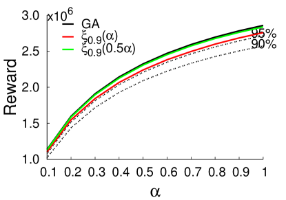
(a) Reward (Weibo)

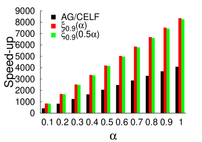
(b) Speed-up (Weibo)

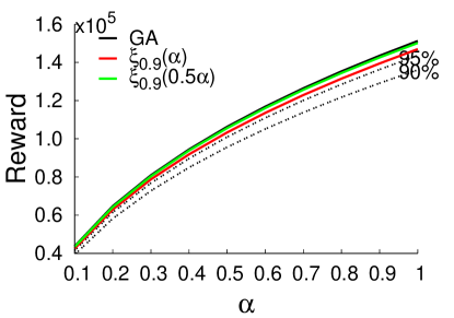
(c) Reward (Twitter)

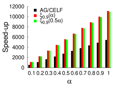
(d) Speed-up (Twitter)

Figure 2: Evaluating the basic framework on real datasets.

Evaluating the vertex sampling framework

Next, we evaluate the benefit of using attribute information within an OSN, in particular, in reducing the size of the candidate set and reducing the computational cost of Alg. 2. For vertex sampling, we consider the following variants: (a) uniformly selecting a node from the network; (b) select a node from the network with a probability proportional to its degree; (c) select the node from the network with a probability proportional to its activity (say # posts). The aim is to select $B=100$ sensors. Each experiment is run 10 times, and the averaged results are shown in Fig. 3. From the reward curves, we observe that vertex sampling by degree is the best follows by sampling by activity, and uniform vertex sampling is the worst. However, from the speed-up curves we can see that uniform vertex sampling is the most efficient approach. Sampling by degree is the most expensive method. But the sampling approaches are in general much more efficient than AG/CELF.

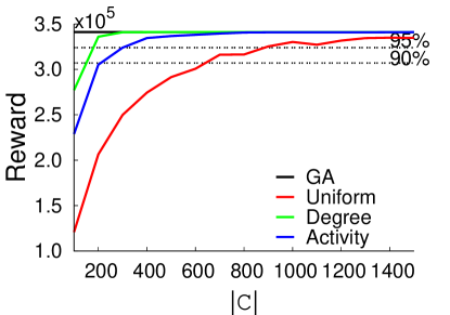
(a) Reward (Weibo)

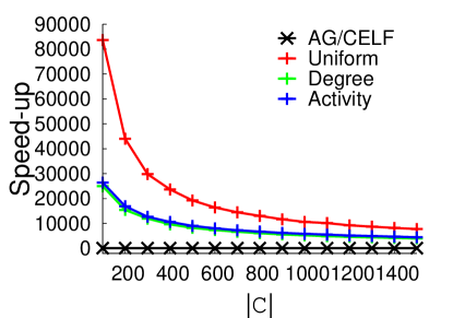
(b) Speed-up (Weibo)

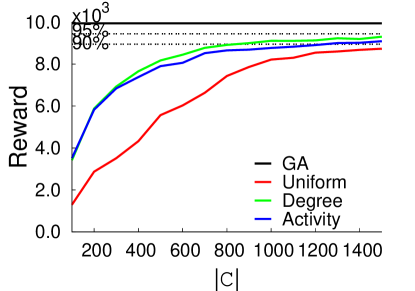
(c) Reward (Twitter)

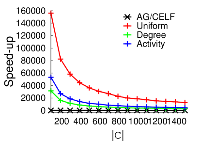
(d) Speed-up (Twitter)

Figure 3: Vertex sampling on real datasets ($B=100$).

Evaluating the random walk framework

We now evaluate the performance of the random walk algorithm as described in Alg. 3. Note that this algorithm does not require the knowledge of the network topology in advance. We have three variants: (a) select a neighboring node uniformly; (b) select a neighboring node with a probability proportional to its degree; (c) select a neigbhoring node with a probability proportional to its activity. The other settings are similar to vertex sampling, and the results are shown in Fig. 4. Again, we can see that degree is the best attribute for random walk, it is also the most expensive one. Comparing random walk with vertex sampling, we observe that random walk can achieve higher accuracy but at a higher computational cost, as is shown in Fig. 5. Both of them are more efficient than AG/CELF. Furthermore, the random walk algorithm does not require a full topology beforehand.

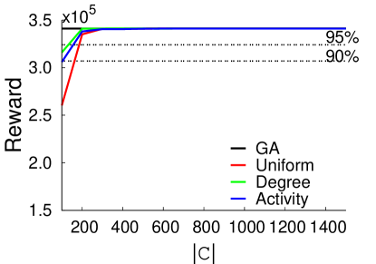
(a) Reward (Weibo)

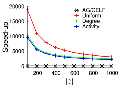
(b) Speed-up (Weibo)

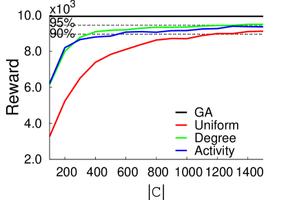
(c) Reward (Twitter)

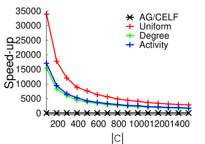
(d) Speed-up (Twitter)

Figure 4: Random walk on real datasets ($B=100$).

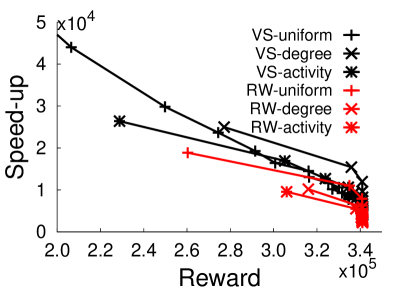
(a) Weibo

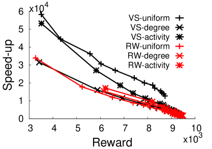
(b) Twitter

Figure 5: Comparing vertex sampling with random walk in Speedup and Reward.

Application Study on Sina Weibo

For a set of selected sensors, we are interested in its detection and prediction capabilities. For detection, it means how many or how timely a set of sensors can discover information cascades from a given dataset. For prediction, it means how well a set of sensors selected based on historical dataset can generalize to a future events, e.g., a set of sensors are selected based on a past week’s data, and we want to know how well they perform on a future week’s data. We conduct experiments on Sina Weibo to study these two capabilities of sensors selected by different methods.

Detection Capability Analysis

We compare the detection quality of our algorithm with two baselines: a) randomly choose a set of nodes as sensors; b) choosing sensors by utilizing friendship paradox(?). Friendship paradox randomly selects a neighbor of a randomly sampled node as a sensor, and it is proved to be able to sample larger degree nodes than random node selection(?).

We then apply the method of Alg. 3 in which random walk is biased by neighbors’ activity and totally 50,000 Weibo accounts are collected, which form the candidate set. We use the posts between Jan 1, 2012 to Sep. 1, 2012 to evaluate the quality of a node. From these candidates we choose $B$ sensors where $B$ ranges from 2,000 to 10,000 using the reward function in Eq. (2). We also introduce two other measures to evaluate sensor quality: (a) the number of cascades sensors can detect; (b) the detecting lead-time, which measures the time interval that the sensors first detect a cascade in advance of the peak time of the cascade. It can be considered as the warning time for outbreaks a set of sensors can provide. The results are shown in Fig. 6. We observe that sensors obtained by Alg. 3 can discover around two to six times more cascades and provide earlier warning time (about two days) than the other two baseline methods.

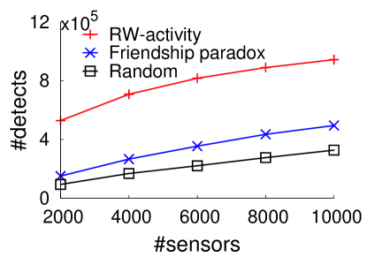
(a) #detects

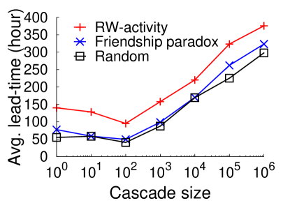
(b) Lead-time

Figure 6: Detection ability comparison.

Prediction Capability Analysis

We study prediction in the scheme of choosing sensors based on historical data and testing them on future data. We want to answer: Are selected sensors based on historical data still good for capturing future cascades? Here we mainly compare the results with the method presented in (?), which chooses sensors using CELF. For our framework, we use Alg. 3 to select the sensor. The Sina Weibo data collected by BFS used in previous section will be our ground truth data, and we split time into granularity of a week.

For the convenience of description, let $T_{i},i\geq 0$ denote the sensors selected by the CELF algorithm using the $i^{th}$ week data. Fig. 7a has two curves: “CELF on week 0” represents running CELF on week $0$ data only, while “CELF on week $i$” represent running CELF on the $i^{th}$ week data. The figure depicts the fraction of cascade detected at different weeks. The black curve corresponds to “CELF on week 0” while the red curve corresponds to “CELF on week $i$”. We can see that the senors in $T_{0}$ (or ”CELF on week 0”) is reducing its predictive capability as time evolves. However, if we use $T_{i}$ (or “CELF on week $i$”), we can have a much higher predictive capability. This implies that social network is highly dynamic and one needs to execute the sensor selection algoirthm more often, rather than relying on sensors selected based on old histrical data.

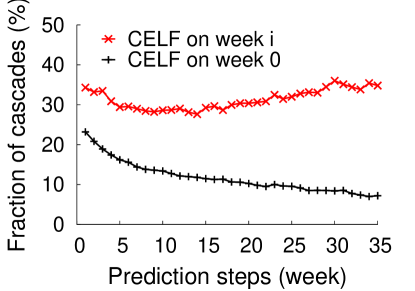
(a) #detects by $T_{0}$ ($B=100$).

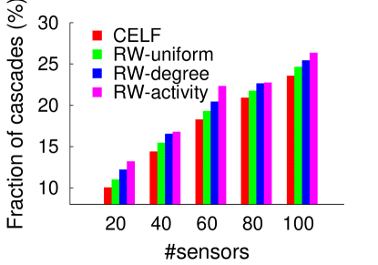
(b) One step prediction.

Figure 7: Prediction ability of sensors.

Next, we study the prediction performance of our method. We choose 1,000 candidates by random walk biased by uniform/degree/activity respectively, from which we select $B$ sensors where $B$ ranges from 20 to 100, and compare the one-week prediction capability with aforementioned “CELF” approach. The result is shown in Fig. 7b. One interesting observation is that our approach is at least as good as the “CELF” approach. Random walk biased by users’ activity is the best, which can improve about 3% of detects on the testing data. Since our approach is more computationally efficient than CELF, hence, one can apply it more often so to have a good predictive capability on information cascade, e.g., better than results of ”CELF on week $i$”.

To understand why our random walk approach has good predictive capability, one can consider the candidate-selecting step as a pruning or regularizing process, which are common techniques used to avoid overfitting of decision trees(?, Chapter 6). For example, when using uniform random walk to collecting candidates, it prefers to select high degree nodes of the network. This can be considered as a rule to regularize the search scope, which can avoid choosing unimportant users who join into large cascades just by chance. To demonstrate this, we use the following regularization rules to constraint search scopes and then apply the CELF to see whether there is any improvements,

• #cascades in a week. The search scope is limited to users who have joined at least $x$ cascades in the history data;

• #active days in a week. The search scope is limited to users who have been active at least $x$ days in the history data;

• #cascades per day. The search scope is limited to users who participates at least $x$ cascades per day.

Fig. 8 depicts the results. We observe some improvements of prediction performance when using different constraints, and users’ activity in history is the best rule, which is consistent with the results in Fig. 7b. This shows that our random walk algorithm has the intrinsic property to regularize the searching scope similar to the above regularization rules.

(a)

(b)

(c)

Figure 8: One step prediction improvements relative to ”greedy” under different regularization rules.

V. Related Work

In this section, we briefly review some related work, which are categorized into three groups:

Influence maximization: One important topic related to our work is how to identify $k$ most influential nodes in a social network. Domingos et al(?) first posed this problem in the area of marketing. Kempe et al(?) proved that the problem is NP-complete under both independent cascade model and threshold model. They also provided an approximation solution which has a constant factor bound. However, computing the influence spread given a seed set by Monte Carlo simulations is not scalable. Other works(?; ?) tried to scale up the Monte Carlo simulation. In our work, we do not assume any cascade or threshold model, but rather, exploit the attributes of OSNs to determine the $B$ sensor nodes.

Optimal sensing: Optimal sensing problems(?; ?) are closely related to our work, which aim to find optimal observers or optimal sensor placement strategies to measure temperature, gas concentration or detect outbreaks in networks(?; ?). Our work can be considered as an extension of Leskovec’s work(?) in which the authors proposed the CELF approach to speedup the greedy algorithm. It is similar to the AG posed by Minoux(?). There are several differences between their work and ours. First, we study the problem without assuming the knowledge on the complete OSN topology. Second, our work aims to speedup the greedy algorithm via graph sampling, and that we can tradeoff a small loss of accuracy but obtain large improvement in efficiency. Furthermore, the performance of our algorithm is guaranteed with high probability. The last property is important since AG/CELF can be as inefficiency as the greedy algorithm in the worst case(?). Third, we exploit the meta information within in social networks. In (?), authors considered the problem as a discrete optimizing problem without considering contextual information in OSNs. In our experiments, we find that contextual information can be used to reduce sample size and improve efficiency.

Graph sampling and optimizing. Graph sampling methods are used to measure properties of nodes and edges in graphs, such as degree distribution(?; ?). To the best of our knowledge, this is the first work which uses graph sampling methods to maximize a set function. Lim et al(?) and Maiya et al(?) both use different sampling methods to estimate the top $k$ largest centrality nodes in a graph, i.e., degree centrality, betweenness centrality, closeness centrality and eigenvector centrality. However these top $k$ largest centrality nodes are not the top $k$ optimal sensors which are defined by a set function $F(\cdot)$. Our work can be considered as a combination of ordinary optimization(?) with greedy algorithm. It uses the property of greedy algorithm that if the reward gain at each round is bounded by factor $\lambda$, then the final solution obtained by the greedy algorithm is bounded by factor $1-1/e^{\lambda}$ as shown in Theorem 1.

VI. Conclusions

Many OSNs are large in scale and there is an urgent need on how to select reliable information sources to subscribe so one can track/detect information cascades. This can be formulated as a sensor placement problem and previous work used heuristic greedy algorithms. However, it is impractical to run these greedy algorithms on a OSN composed of millions of users. Hence we propose sampling approach to find these good sensors.

We show that one can significantly reduce the complexity by sampling the huge search space, and still can guarantee to have good solutions with high probabilistic guarantees. Hence, the sampling approach is a good method to trade off efficiency and accuracy. We evaluate various graph sampling approaches, and find that random walk based sampling methods perform better than vertex sampling based methods. This indicates that structural information of OSNs is important and random walks are suitable for obtaining better samples, while previous discrete optimization approaches failed to utilize this information. We apply our framework on Sina Weibo, and the results demonstrate that using our algorithm, one can effectively detect information cascade. Since our algorithm is computationally efficient, one can execute it more often so to find new sensor nodes to accurately predict future information cascade.

Appendix

Proof of Theorem 1

Proof.

By utilizing the non-decreasing property of $F$, we have

$$F(OPT)-F(S_{k-1})\leq F(OPT\cup S_{k-1})-F(S_{k-1})$$

$$= F(OPT\backslash S_{k-1}\cup S_{k-1})-F(S_{k-1}).$$

Assume $OPT\backslash S_{k-1}=\{z_{1},\cdots,z_{m}\},m\leq K$, and let $j=1,\cdots,m$, we have

$$Z_{j}=F(S_{k-1}\cup\{z_{1},\cdots,z_{j}\})-F(S_{k-1}\cup\{z_{1},\cdots,z_{j-1}\}).$$

With some algebraic manipulation, we have

$$F(OPT)-F(S_{k-1})\leq\sum_{j=1}^{m}Z_{j}.$$

Now notice that

$$Z_{j}\leq F(S_{k-1}\cup\{z_{j}\})-F(S_{k-1})$$

$$= \delta_{z_{j}}(S_{k-1})\leq\frac{1}{\lambda}\delta_{\hat{s}_{k}^{*}}(S_{k-1})$$

$$= \frac{1}{\lambda}(F(S_{k})-F(S_{k-1})).$$

Then we get an iterative formula of $F(S_{k})$,

$$F(OPT)-F(S_{k-1})\leq\sum_{j=1}^{m}Z_{j}\leq\frac{K}{\lambda}(F(S_{k})-F(S_{k-1})).$$

Iteratively, we can derive the following relationship,

$$F(S_{k})\geq[1-(1-\frac{\lambda}{K})^{k}]F(OPT).$$

Finally, let $k=K$. We conclude that

$$F(S_{K})\geq[1-(1-\frac{\lambda}{K})^{K}]F(OPT)\geq(1-\frac{1}{e^{\lambda}})F(OPT).$$

∎

Proof of Theorem 2

Proof.

Let $y_{i}$ denote the number of nodes in $OPT$ that have been covered after the $i$-th round and $\bar{y}_{i}$ be its expectation. Further, let $q_{i}$ denote the probability that an uncovered node in $OPT$ will be covered in the $i$-th round. Then the expectation of $y_{i}$ is

$$\bar{y}_{i}=\bar{y}_{i-1}+q_{i},$$ (9)

For $\alpha\%=K/|V|$ and confidence $p$, we are pretty sure that one of the $K$ nodes will fall in $\xi_{p}(\alpha)$ with probability at least $p$. Hence, the probability of sampling an uncovered node of $OPT$ in round $i$ is

$$q_{i}\geq p\frac{K-\bar{y}_{i-1}}{K}.$$

Substituting the above equation into Eq. (9), we get

$$\bar{y}_{i}\geq\bar{y}_{i-1}+p\frac{K-\bar{y}_{i-1}}{K}.$$

Iteratively, it can be written in the following form,

$$\bar{y}_{i}\geq(1-\frac{p}{K})^{i}\bar{y}_{0}+K[1-(1-\frac{p}{K})^{i}]$$

Since $\bar{y}_{0}=0$, we get

$$\bar{y}_{i}\geq K[1-(1-\frac{p}{K})^{i}].$$

After the $K$-th round, we conclude

$$\mathbb{E}[r]=\frac{\bar{y}_{K}}{K}\geq 1-(1-\frac{p}{K})^{K}\geq 1-\frac{1}{e^{p}}.$$

∎

References

- [Chen, Wang, and Yang 2009] Chen, W.; Wang, Y.; and Yang, S. 2009. Efficient influence maximization in social networks. In KDD’09, 199–208.
- [Christakis and Fowler 2010] Christakis, N. A., and Fowler, J. H. 2010. Social network sensors for early detection of contagious outbreaks. PLoS ONE 5.
- [Domingos and Richardson 2001] Domingos, P., and Richardson, M. 2001. Mining the network value of customers. In KDD’01.
- [Feld 1991] Feld, S. L. 1991. Why your friends have more friends than you do. American Journal of Sociology 96(6):1464–1477.
- [Fujito 2000] Fujito, T. 2000. Approximation algorithms for submodular set cover with applications. IEICE TRANS. INF. & SYST.
- [Ho, Sreenivas, and Vakili 1992] Ho, Y. C.; Sreenivas, R. S.; and Vakili, P. 1992. Ordinal optimization of deds. Discrete Event Dynamic Systems: Theory and Applications 2:61–88.
- [Kempe, Kleinberg, and Tardos 2003] Kempe, D.; Kleinberg, J.; and Tardos, E. 2003. Maximizing the spread of influence through a social network. KDD’03.
- [Khuller, Moss, and Naor 1999] Khuller, S.; Moss, A.; and Naor, J. S. 1999. The budgeted maximum coverage problem. Information Processing Letters 70:39–45.
- [Krause 2008] Krause, A. 2008. Optimizing Sensing Theory and Applications. Ph.D. Dissertation, School of Computer Science Carnegie Mellon University.
- [Leskovec et al. 2007] Leskovec, J.; Krause, A.; Guestrin, C.; Faloutsos, C.; VanBriesen, J.; and Glance, N. 2007. Cost-effective outbreak detection in networks. KDD’07 420–429.
- [Li, qiao Zhao, and Lui 2012] Li, Y.; qiao Zhao, B.; and Lui, J. C. 2012. On modeling product advertisement in large scale online social networks. IEEE/ACM Transitions on Networking.
- [Lim et al. 2011] Lim, Y.; Ribeiro, B.; Menasch´e, D. S.; Basu, P.; and Towsley, D. 2011. Online estimating the top k nodes of a network. IEEE NSW.
- [Link 2010] 2010. What is twitter, a social network or a news media? http://an.kaist.ac.kr/traces/WWW2010.html.
- [Link 2011] 2011. 476 million twitter tweets. http://snap.stanford.edu/data/twitter7.html.
- [LOVASZ 1993] LOVASZ, L. 1993. Random walks on graphs: A survey. BOLYAI SOCIETY MATHEMATICAL STUDIES 1–46.
- [Maiya and Berger-Wolf 2010] Maiya, A. S., and Berger-Wolf, T. Y. 2010. Online sampling of high centrality individuals in social networks. PAKDD.
- [Minoux 1978] Minoux, M. 1978. Accelerated greedy algorithms for maximizing submodular set functions. Optimization Techniques.
- [Nemhauser, Wolsey, and Fisher 1978] Nemhauser, G. L.; Wolsey, L. A.; and Fisher, M. L. 1978. An analysis of approximations for maximizing submodular set functions. Mathematical Programming 14:265–294.
- [Ribeiro and Towsley 2010] Ribeiro, B., and Towsley, D. 2010. Estimating and sampling graphs with multidimensional random walks. IMC’10.
- [Witten and Frank 2005] Witten, I. H., and Frank, E. 2005. Data Mining: Practical Machine Learning Tools and Techniques. Morgan Kaufmann.