Capacity Value of Additional Generation: Probability Theory and Sampling Uncertainty

Abstract

The concept of capacity value is widely used to quantify the contribution of additional generation (most notably renewables) within generation adequacy assessments. This paper surveys the existing probability theory of assessment of the capacity value of additional generation, and discusses the available statistical estimation methods for risk measures which depend on the joint distribution of demand and available additional capacity (with particular reference to wind).

Preliminary results are presented on assessment of sampling uncertainty in hindcast LOLE and capacity value calculations, using bootstrap resampling. These results indicate strongly that, if the hindcast calculation is dominated by extremes of demand minus wind, there is very large sampling uncertainty in the results due to very limited historic experience of high demands coincident with poor wind resource. For meaningful calculations, some form of statistical smoothing will therefore be required in distribution estimation.

I Introduction

The concept of capacity value is widely used to quantify the contribution of variable output renewable generation technologies within generation adequacy assessments. Common specific definitions include Effective Load Carrying Capability (ELCC, the extra demand which the additional generation can support without increasing the chosen risk metric), and Equivalent Firm Capacity (EFC, the completely firm conventional capacity which would give the same risk level if it replaced the additional variable generation). These are usually calculated with respect to adequacy risk indices such as the Loss of Load Probability (LOLP) at time of annual peak, or the Loss of Load Expectation (LOLE, the sum over periods of LOLP, or equivalently the expected number of periods of shortage in a given time window).

There are many surveys in the literature of capacity value calculation methods, for instance [1, 2, 3]. In addition, a number of papers have been published recently on analytical calculation approaches which are valid for small additional capacities [4, 5], or for the special case where the distribution of margin of existing capacity over demand has an exponential tail [6, 7]; these analytical approaches are surveyed in [8]. [9] and [10] provide general surveys of adequacy assessment methods. The website of the IEEE PES LOLE Working Group contains many useful presentations on current industrial adequacy assessment practices [11].

This paper will provide a comprehensive survey of the existing probability theory of capacity value calculations (Section II). In particular, this formulates the theory in terms of the distributions of available additional capacity and of margin of available conventional capacity over demand, which simplifies much of the mathematical exposition and clarifies exactly what features of distributions drive the capacity value results. Section III then discusses the statistical methods for estimating the inputs to these calculations, and in particular proposes bootstrap resampling as a means of estimating sampling uncertainty in capacity value and LOLE calculation results. Data for illustrative examples is provided in Section IV, then Section V presents examples of uncertainty assessment. While we do not claim to be presenting a quantitative adequacy assessment for the Great Britain system, some conclusions may be drawn regarding the degree of uncertainty in results produce by the common hindcast approach. Finally conclusions are presented in Section VI.

II Probability Theory of Capacity Values

We present first a “snapshot” picture of the theory, appropriate to the distributions of the variables involved at a given instant of time. We then consider how this generalises to extended periods of time such a year.

II-A Snapshot Theory: Definitions

Suppose that existing capacity less demand is represented by a random variable $M$, with distribution function $F_{M}$ and density function $f_{M}$.

The capacity value of additional generation represented by a random variable $Y$ is in some appropriate sense a deterministic capacity which is equivalent to it in terms of an associated risk. In general it may be viewed as the mean of $Y$ less some correction which corresponds to its variability.

Suppose that $Y\geq 0$ with distribution function $F_{Y}$ and density function $f_{Y}$. We denote its mean and variance by $\mu_{Y}$ and $\sigma^{2}_{Y}$ respectively.

The two most commonly used definitions of the capacity value of $Y$ are:

Effective Load Carrying Capability (ELCC): This is given by the solution $\nu^{\mathrm{ELCC}}_{Y}$ of

$$\mathbf{P}(M+Y\leq\nu^{\mathrm{ELCC}}_{Y})=\mathbf{P}(M\leq 0)=F_{M}(0),$$ (1)

i.e. the amount of further demand which may be added while maintaining the same level of risk.

Equivalent Firm Capacity (EFC): This is given by the solution $\nu^{\mathrm{EFC}}_{Y}$ of

$$\mathbf{P}(M+Y\leq 0)=\mathbf{P}(M+\nu^{\mathrm{EFC}}_{Y}\leq 0)=F_{M}(-\nu^{\mathrm{EFC}}_{Y}),$$ (2)

i.e. the amount of deterministic capacity $\nu^{\mathrm{EFC}}_{Y}$ whose addition would result in the same level of risk as that of the addition of the random capacity $Y$.

It is important to note that both $\nu^{\mathrm{ELCC}}_{Y}$ and $\nu^{\mathrm{EFC}}_{Y}$ depend on the distributions of both $M$ and $Y$. Note also that in the case where $Y$ is deterministic ($Y=\mu_{Y}$ always) we have $\nu^{\mathrm{EFC}}_{Y}=\nu^{\mathrm{ELCC}}_{Y}=\mu_{Y}$.

We consider first the case where $M$ and $Y$ are independent, and then discuss what modifications are required to deal with the more general case.

II-B The case where $M$ and $Y$ are independent

Assume that $M$ and $Y$ are independent. Consider first two special cases, both of which are analytically tractable and inform the general case.

II-B1 Small additional capacity

The first case is where the variation in $Y$ is small in relation to that in $M$ and was considered in [4]. Result 1 of that paper showed that, to a good approximation,

$$\nu^{\mathrm{EFC}}_{Y}=\nu^{\mathrm{ELCC}}_{Y}=\mu_{Y}-\frac{f_{M}^{\prime}(0)}{2f_{M}(0)}\sigma_{Y}^{2},$$ (3)

where the error is negligible in relation to $\sigma_{Y}^{2}$ as the latter becomes small (in relation to the variation in $M$). We also see here that capacity values of small independent additions are additive, i.e. if $M$, $Y_{1}$ and $Y_{2}$ are independent random variables, and if $Y=Y_{1}+Y_{2}$, then (since $\mu_{Y}=\mu_{Y_{1}}+\mu_{Y_{2}}$ and $\sigma^{2}_{Y}=\sigma^{2}_{Y_{1}}+\sigma^{2}_{Y_{2}}$) it follows from (3) that $\nu^{\mathrm{EFC}}_{Y}=\nu^{\mathrm{EFC}}_{Y_{1}}+\nu^{\mathrm{EFC}}_{Y_{2}}$ (and similarly for $\nu^{\mathrm{ELCC}}_{Y}$).

II-B2 Exponential left tail for $M$ (‘Garver approximation’)

The second case. which forms the basis of the well-known Garver approximation [6, 7], arises when the distribution function $F_{M}$ of $M$ may be treated as exponential below some level $m_{0}$, i.e. $F_{M}(m)=c\exp\lambda_{M}m$ for $m\leq m_{0}$ for some $\lambda_{M}>0$. Then, since $Y\geq 0$ is independent of $M$, it is easily checked that the distribution of $M+Y$ is similarly exponential below the level $m_{0}$, i.e. for $m\leq m_{0}$,

$$\mathbf{P}(M+Y\leq m) =\int_{0}^{\infty}\mathrm{d}yf_{Y}(y)F_{M}(m-y)$$

$$=ce^{\lambda_{M}m}\int_{0}^{\infty}\mathrm{d}yf_{Y}(y)e^{-\lambda_{M}y}$$

$$=\mathbf{P}(M+\nu\leq m),$$ (4)

where $\nu$ is the solution of

$$\mathbf{E}\exp(-\lambda_{M}Y)=\int_{0}^{\infty}\mathrm{d}yf_{Y}(y)e^{-\lambda_{M}y}=\exp(-\lambda_{M}\nu).$$ (5)

and $\mathbf{E}$ denotes expectation.

It follows that, provided we can take $m_{0}\geq 0$ (in the case of the EFC) and $m_{0}\geq\nu^{\mathrm{ELCC}}_{Y}$ (in the case of the ELCC), the commonly used capacity measures $\nu^{\mathrm{ELCC}}_{Y}$ and $\nu^{\mathrm{EFC}}_{Y}$ are each equal to $\nu$ here. Further, in this case the capacity value depends on the distribution of $Y$ through its Laplace transform evaluated at $\lambda_{M}$, so that we may readily study which features of this distribution influence the capacity value. The essentials of this derivation of the Garver approximation are not new, however the notation of this paper makes the working much more concise than previous versions such as [7].

Finally it follows from the standard result for the Laplace transform of the sum of independent random variables that (as in the earlier case where the variation in $Y$ is small) capacity values of independent additions are additive.

II-B3 The general case

In the more general case, when the above exponential approximation of $F_{M}$ is not necessarily available, the equation (2) may be written as

$$\int_{0}^{\infty}\mathrm{d}y\,f_{Y}(y)F_{M}(-y)=F_{M}(-\nu^{\mathrm{EFC}}_{Y})$$ (6)

using the standard result for the convolution of two independent random variables (a similar expression holds for the ELCC). This may be solved by standard numerical techniques.

II-C The case where $M$ and $Y$ may be dependent

If independence of $M$ and $Y$ is not assumed, then capacity values must typically be determined by reference to (1) or (2). We discuss this further in Section III. However, when the variation in the distribution of the additional capacity $Y$ is significantly less than that in the distribution of $M$ then the equation (2) may still be approximated by (3) provided the density $f_{Y}(y)$ of $Y$ is replaced by its conditional density given $M=0$ (this corresponds to the assertion that for values of $M$ within the critical region, i.e. in the neighbourhood of $M=0$, the conditional density of $Y$ does not vary significantly). Except for this relatively straightforward adjustment, the preceding theory remains as before.

II-D Application to extended periods of time

Typically a capacity value is required for a period of time such as a year, which may be represented as being composed of a sequence of much shorter periods of time, typically of hours or half-hours, to each of which the above “snapshot” picture is applicable. We index these shorter periods by $t$, and the random variables $M_{t}$ and $Y_{t}$ are respectively the surplus $M$ and additional capacity $Y$ during period $t$ (their distributions typically varying with $t$).

For simplicity consider the EFC $\nu^{\mathrm{EFC}}_{Y}$. The equation (2) is now replaced by

$$\sum_{t}\mathbf{P}(M_{t}+Y_{t}\leq 0)=\sum_{t}\mathbf{P}(M_{t}+\nu^{\mathrm{EFC}}_{Y}\leq 0)$$ (7)

i.e. $\nu^{\mathrm{EFC}}_{Y}$ is the deterministic completely firm generating capacity if the same loss of load expectation is to be maintained as in the case with additional stochastic capacity $Y$. In the case where the pairs $(M_{t},Y_{t})$ are viewed as corresponding to randomly chosen periods of time and are thus treated as identically distributed (with the ‘whole peak season’ distribution), the equation (7) does of course reduce to (2).

III Statistical estimation

Throughout this section we consider, for definiteness, the estimation of the EFC $\nu^{\mathrm{EFC}}_{Y}$.

Approaches to statistical estimation naturally depend on the nature of the available data. In the present paper we assume that the random variable $M=X-D$ where $X$ is existing, typically conventional, capacity and $D$ is demand. We further assume that the successive instances of $X$, i.e. the random variables $X_{t}$, may be modelled as identically distributed, with a known distribution function $F_{X}$ (typically determined from a capacity outage table), and are independent of the random variables $D_{t}$ and $Y_{t}$. We thus rewrite the equation (7) as

$$\sum_{t}\mathbf{E}F_{X}(D_{t}-Y_{t})=\sum_{t}\mathbf{E}F_{X}(D_{t}-\nu^{\mathrm{EFC}}_{Y}).$$ (8)

This formulation incorporates the above independence assumption, and is thus most suited to inference given observations $(d_{t},y_{t})$ of the successive pairs $(D_{t},Y_{t})$. (We here assume that the joint distribution of the pairs $(D_{t},Y_{t})$ is to be estimated from data, as will be the case when the additional capacity $Y$ corresponds to some renewable resource such as wind generation.)

Further assumptions (often not made explicit in the existing literature) are now necessary in order to make any inference for $\nu^{\mathrm{EFC}}_{Y}$. Usually we treat the pairs $(D_{t},\,Y_{t})$ as identically distributed—with the ‘whole peak season’ distribution referred to in the previous section—and we henceforth assume this, representing this common distribution as that of a generic pair $(D,\,Y)$. Point estimates of $\nu^{\mathrm{EFC}}_{Y}$ do not then in general require any assumptions about the nature of any dependence between the successive pairs $(D_{t},Y_{t})$. Assessments of uncertainty for these estimates, e.g. confidence intervals, do require such assumptions. The simplest such is to take the pairs $(D_{t},Y_{t})$ to be additionally independent, thus allowing straightforward techniques to be used for the construction of confidence intervals, etc. However, in reality significant serial correlations will be present; correctly allowing for these (which may require data of better quality than is currently available) will significantly increase the reported uncertainty associated with estimates of $\nu^{\mathrm{EFC}}_{Y}$.

Finally, while it will be typically be unrealistic to assume independence of the generic $D$ and $Y$ (since, for example, demand and available wind will typically have some statistical association), we make nevertheless wish to make some smoothness assumptions concerning the nature of the dependence between them. We discuss this further below.

The simplest approach to the estimation of $\nu^{\mathrm{EFC}}_{Y}$ is to substitute the observed values $(d_{t},\,y_{t})$ of $(D_{t},\,Y_{t})$ into (8), giving the expression

$$\sum_{t}F_{X}(d_{t}-y_{t})=\sum_{t}F_{X}(d_{t}-\nu^{\mathrm{EFC}}_{Y}).$$ (9)

(where the sum is over the historic times $t$ for which data is available) and to solve for $\nu^{\mathrm{EFC}}_{Y}$. This is the commonly used hindcast approach, and has the virtue of making no assumptions about the common joint distribution of $(D,\,Y)$. (In particular it attempts to account for statistical association between $D$ and $Y$ in the historic data without requiring any advanced statistical technology). A common criticism of the approach relates to the difficult of making an uncertainty assessment of the estimate for $\nu^{\mathrm{EFC}}_{Y}$; indeed results are usually presented without assessment of uncertainty. However, under the additional independent assumption for the successive pairs $(D_{t},\,Y_{t})$ referred to above, the latter may be obtained easily by bootstrapping (successively resampling from the data) [12, 13].

A major difficulty with the simple hindcast approach described above is the likely shortage of data in the extreme regions of relevance to the solution of (8) (or (9)), leading to considerable uncertainty in the estimate of $\nu^{\mathrm{EFC}}_{Y}$. This can be partially remedied by assuming some reasonably smooth form of dependence in the joint distribution of $(D,\,Y)$—an assumption which effectively allows more observations to make a helpful contribution to the estimation procedure. The most radical such assumption is to take $D$ and $Y$ to be independent, but this will typically be unrealistic: for example, to the extent that wind and demand are typically both higher in winter, there is a positive statistical association between them.

A sensible compromise is to indeed proceed as if the demand $D$ and additional capacity $Y$ were independent, but to replace the distribution of $Y$ by an estimate of its conditional distribution given that the demand $D$ lies within the region critical for the estimation of $\nu^{\mathrm{EFC}}_{Y}$. In practice this means treating $D$ and $Y$ as independent but replacing the distribution of $Y$ by its distribution for those times—of the year and of the day—in which the modelled system is at risk, i.e. in which the demand $D$ tends to be high. (In the case where $Y$ is wind generation, an interesting alternative is to use a distribution of $Y$ estimated using data from those classes of weather system for which demand $D$ is likely to be high [14]; however care is required here as it may be that types of weather for which demand is less extreme may also be associated with particularly low levels of wind, again placing the system at risk.) From (8) and our “identically distributed” assumption, estimation of $\nu^{\mathrm{EFC}}_{Y}$ now reduces to the solution of

$$\mathbf{E}F_{X}(D-Y)=\mathbf{E}F_{X}(D-\nu^{\mathrm{EFC}}_{Y}).$$ (10)

where $D$ and $Y$ are additionally treated as independent with distributions as suggested by the data sampled at the critical periods referred to above. These may be the relevant empirical distributions, perhaps smoothed, in which case the solution of (10) will necessarily be numerical; alternatively parametric estimates of these distributions may be used. In the former case assessments of uncertainty may be made by bootstrap resampling using each of the two empirical distributions; in the latter either bootstrap or analytical techniques may be used.

IV Data for Examples

This section describes the Great Britain-based test data used for calculation examples in this paper. The descriptions are quite brief, as this paper does not claim to perform a quantitative capacity value study for this system. Instead, it illustrates the ideas on uncertainty assessment by bootstrapping described above, and provides an indication of the degree of uncertainty which may be observed in more definitive calculations.

IV-A Conventional Plant

The probability distribution of available conventional capacity is based on the list of units connected to the GB system in winter 2008/09. A standard capacity outage probability table (COPT) calculation is performed, with the availability probabilities for each class of generating unit taken from [15]; in a small number of cases, the maximum contribution from each station is capped due to finite network capacity or emissions constraints, following the practice of the GB system operator. In all examples, the distributions of available conventional capacity at different times are assumed to be identically distributed. This is reasonable if there is little planned maintenance at times when risk is high, and hence all units that are mechanically available are available to generate if required.

For the illustrative examples presented here, the distribution of available conventional capacity will not be rescaled; instead the peak demand will be adjusted to achieve a risk level consistent with historic experience. This will allow general conclusions to be drawn regarding the the importance of uncertainty analysis, but a more careful treatment of the conventional plant is clearly required in practical risk calculations (and associated assessment of uncertainty).

IV-B Demand Data

Half-hourly historic transmission-metered demand data is available for the GB system since April 2001 [16]. This paper uses the seven years 2002-8 for which coincident wind resource data is also available; as the wind data is hourly, for each hour the demand used is the higher demand from the two half hours contained therein. Historic demands from different years may be compared to an extent by rescaling according to each winter’s Average Cold Spell (ACS) peak demand metric, although this does not account fully for changes in underlying demand patterns (including increasing penetrations of distributed generation). The ACS peak level for each winter is published by the GB System Operator.

IV-C Wind Data

The wind resource data used in this paper was generated by Pöyry Consulting for their ‘Impact of Intermittency’ report; a more detailed description of the dataset may be found in [18]. This dataset is based on hourly wind speed records from 19 onshore meteorological stations around GB, plus 7 offshore locations where the historic data is derived by atmospheric modelling. As described above, these observations are coincident in time with the demand data from 2002-8. These wind speed time series are transformed to wind load factors using a generic wind farm power curve, and the resulting load factor time series from each of these sites is assumed to be representative of wind farms in that area. Finally a time series of system aggregate wind power outputs are generated for a 2020 scenario of installed wind capacities.

We note a number of uncertainties associated with this data, including how representative the chosen locations are of actual wind farm locations, some issues of limited geographical coverage (notably including a total lack of data from Scottish offshore waters) and conversion of wind speed data to hub height wind speeds and then wind power. For quantitative applied studies, we believe that the most satisfactory approach to wind resource modelling is mesoscale reanalysis, in which physical atmospheric modelling is used to downscale a coarse-grid historic record to the spatial and temporal resolution required for the power system analysis work [19].

V Assessment of Uncertainty

This section demonstrates how bootstrap resampling, mentioned in Section III, can provide an estimate of statistical uncertainty in hindcast LOLE and EFC calculations. Bootstrap brings the key advantage over the previous method in [20] that it does not require an assumed ‘correct’ result for comparison in order to make a quantification of statistical uncertainty. As described in IV, we do not claim that this paper provides a quantitative LOLE or capacity value assessment for the GB system. However, the consideration of uncertainty in our example calculations will permit important conclusions about statistical methodologies for practical adequacy assessment.

For this illustrative purpose, all calculations are performed with ACS peak demand of 61.5 GW and the conventional plant distribution described above. This underlying demand level gives, for all wind capacities considered, a highest hourly LOLP in the hindcast LOLE calculation (i.e. largest term in the sum on the right hand side of (9)) of the order of 1%; a risk level of this order is widely reckoned to be economically sustainable in GB. The hindcast calculation utilises only those observations $(d_{t},\,y_{t})$ corresponding to the 5000 highest values of $d_{t}$, and constituting 8% of the total data. (For the remaining observations $d_{t}$ is insufficiently high to make any contribution to the solution of (9).)

V-A Uncertainty in Hindcast LOLE and EFC

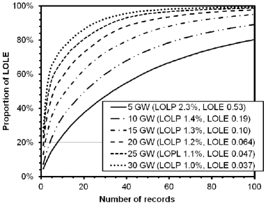
Figure 1: Proportion of LOLE arising from the top $n$ net demands in the right hand side of (9), for a range of installed wind capacities. The LOLE figures quoted are in hours per seven years (based on the seven years of data used. The LOLP figure is the highest hourly LOLP in the sum on the RHS of (9).

The part of the calculated LOLE due to the $n$ historic records with the highest net demands is shown in Fig. 1 for a range of installed wind capacties (i.e.

$$\sum_{t=1}^{n}F_{X}(d_{t}-y_{t})$$ (11)

where the times $t$ are ordered by decreasing net demand $d_{t}-y_{t}$). This is expressed as a proportion of the total LOLE where all data is included in the sum.

An indication of uncertainty in results for a range of wind capacities is obtained by simple rescaling of the wind power data from the 2020 scenario on which the time series is based. It may be seen that at high wind capacities, the calculation becomes dominated by a very small number of records with high demand and poor wind resource. Indeed, for 30 GW installed wind capacity, 67% of the calculated LOLE is due to records from just two consecutive days in February 2006. It is clear that in such a situation the calculation will have very limited ability to estimate risk at future times.

Fig. 2 shows the distribution of calculated LOLEs arising from 200 bootstrap samples from the historic joint series of demand and available wind capacity. Each bootstrap sample is a random sample of the same size as that of the original dataset (of size 5000 as described above), sampled from the empirical distribution of the that dataset. The distribution of the calculated LOLEs of the 200 bootstrap samples constitutes a direct assessment of the sampling distribution of the LOLE for the original data. The calculations are repeated for a range of installed wind capacities. In making this assessments, the demand-wind pairs at different times are assumed to be independent and identically distributed. In reality there are important serial associations between consecutive hours and days, and this estimate of uncertainty based on the assumption of independence will thus be an underestimate.

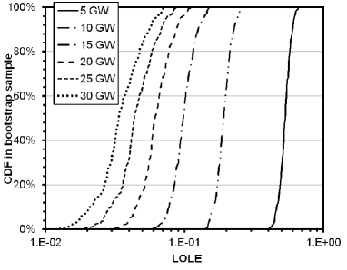
Figure 2: Distribution of LOLE results arising from 200 bootstrap samples from the historic time series of wind and demand, for a range of installed wind capacities.

Even for only 5 GW of installed wind capacity, the 95% confidence intervals for the LOLE arising from the bootstrap analysis ranges from 0.44 to 0.62, a factor of 1.4. However, for 30 GW installed capacity, the confidence interval covers the range 0.016 to 0.068, a factor of 4.2.

The distributions of EFC results arising from similar bootstrap resampling are shown in Fig. 3. The apparent greater robustness of the EFC results (as compared to those for LOLE) arising from these bootstrap calculations is merely a consequence of the nonlinear rescaling of the risk level to a MW capacity value by inverting the cumulative distribution function of $M$.

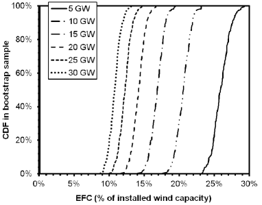
Figure 3: Distribution of EFC results arising from 200 bootstrap samples from the historic time series of wind and demand, for a range of installed wind capacities.

V-B Discussion

As stated previously, these calculations are primarily intended to illustrate the proposed statistical methodologies, and certainly do not constitute a quantitative adequacy assessment for the Great Britain system. The latter is planned by the authors as future work, and will require improved data, including realistic scenarios of installed generating capacity for the future years under study.

Nevertheless, some important conclusions can be drawn from this initial study. The first is that a hindcast LOLE calculation for the GB system with a high installed wind capacity can say very little meaningful about real risk levels. This is demonstrated clearly by the tiny number of historic days’ data which dominate the calculation, and by the bootstrap results. The latter in particular give an optimistic view of the degree of uncertainty due to the modelling of demand-wind pairs at different times as independent and identically distributed.

Section III describes how sampling uncertainty might be reduced by some form of statistical smoothing. This might be relatively straightforward as described there, or might involve application of extreme value statistical methods. While such approaches will certainly reduce sampling uncertainty, there will remain some (hopefully modest) additional uncertainty over the applicability of the chosen methodology.

Future work on bootstrap assessment of uncertainty in hindcast calculations should include consideration of serial associations in the time series of demand and wind conditions. This will be required for any hindcast calculations performed in GB for relatively modest wind capacities (where the sampling uncertainty is not overwhelming), and also for other systems where the risk calculation results are not dominated to the same extent by a small number of extremes of net demand in the historic data.

VI Conclusion

This paper has surveyed the existing probability theory of assessment of the capacity value of additional generation, and discussed the available statistical estimation methods for risk measures which depend on the joint distribution of demand and available additional capacity (with particular reference to wind).

Preliminary results have been presented on assessment of sampling uncertainty in hindcast LOLE and capacity value calculations, using bootstrap resampling. The test system used is not sufficiently realistic as to provide a quantitative generation adequacy risk study for the Great Britain system. Nevertheless, the results indicate strongly that, in systems such as GB where the calculated adequacy risk is dominated by extremes of demand minus wind, there is very large sampling uncertainty in hindcast adequacy calculation results due to limited historic experience of high demands coincident with poor wind resource. For meaningful calculations, some form of statistical smoothing will therefore be required in estimation. The results also confirm that uncertainty analysis is a vital part of any generation adequacy study, particular in systems with a substantial wind generation capacity.

References

- [1] A. Keane, M. Milligan, C. J. Dent, B. Hasche, C. D’Annunzio, K. Dragoon, H. Holttinen, N. Samaan, L. Söder, and M. O’Malley, “Capacity Value of Wind Power,” IEEE Trans. Power Syst., vol. 26, no. 2, pp. 564–572, 2011, IEEE PES Task Force report.
- [2] M. Amelin, “Comparison of Capacity Credit Calculation Methods for Conventional Power Plants and Wind Power,” IEEE Trans. Power Syst., vol. 24, no. 2, pp. 685–691, May 2009.
-
[3]
NERC Integration of Variable Generation Task Force, “Methods to Model
Calculate Capacity Contributions of Variable Generation for Resource Adequacy
Planning,” 2011, available at
http://www.nerc.com/filez/ivgtf_Probabilistic.html. - [4] S. Zachary and C. J. Dent, “Probability theory of capacity value of additional generation,” 2011, J. Risk and Reliability (Proc. IMechE pt. O), in press.
- [5] K. Dragoon and V. Dvortsov, “Z-Method for Power System Resource Adequacy Applications,” IEEE Trans. Power Syst., vol. 21, no. 2, May 2006.
- [6] L. L. Garver, “Effective load carrying capability of generating units,” IEEE Trans. Power Apparatus and Systems, vol. 85, no. 8, pp. 910–919, August 1966.
- [7] C. D’Annunzio and S. Santoso, “Noniterative method to approximate the effective load carrying capability of a wind plant,” IEEE Trans. Energy Conv., vol. 23, no. 2, pp. 544–550, June 2008.
- [8] C. J. Dent, A. Keane, and J. W. Bialek, “Simplified Methods for Renewable Generation Capacity Credit Calculation: A Critical Review,” in IEEE PES General Meeting, 2010.
- [9] R. Billinton and R. N. Allan, Reliability evaluation of power systems, 2nd edition. Plenum, 1994.
- [10] W. Li, Risk Assessment of Power Systems: Models, Methods, and Applications. IEEE/Wiley, 2005.
-
[11]
IEEE PES LOLE WG meeting, 7-8 November 2011, available at
http://ewh.ieee.org/cmte/pes/rrpa/RRPA_20111107LBPmtg.html. - [12] B. Efron, “Bootstrap Methods: Another Look at the Jackknife,” Annals of Statistics, vol. 7, no. 1, pp. 1–26, 1979.
- [13] B. Efron and R. Tibshirani, An introduction to the bootstrap. Chapman and Hall, 1993.
- [14] D. J. Brayshaw, C. J. Dent, and S. Zachary, “Wind generation’s contribution to supporting peak electricity demand: meteorological insights,” 2011, J. Risk and Reliability (Proc. IMechE pt. O), in press.
- [15] National Grid, “Winter Outlook Report 2010/11,” 7 October 2010, available from http://www.nationalgrid.com/uk/Gas/TYS/outlook/.
-
[16]
“National Grid: Demand Data,” available at
http://www.nationalgrid.com/uk/Electricity/Data/Demand+Data/. -
[17]
“Great Britain National Electricity Transmission System Security and Quality
of Supply Standard, Issue 2.0,” 24 June 2009, available from
http://www.nationalgrid.com/uk/Electricity/Codes/
gbsqsscode/DocLibrary/. - [18] Pöyry Energy Consulting, “Impact of Intermittency: Summary Report,” July 2009.
- [19] D. Lew, C. Alonge, M. Brower, J. Frank, L. Freeman, K. Orwig, C. Potter, and Y.-H. Wan, “Wind Data Inputs for Regional Integration Studies,” in IEEE PES General Meeting, 2011, p. 1097.
- [20] B. Hasche, A. Keane, and M. O’Malley, “Capacity Value of Wind Power, Calculation and Data Requirements: the Irish Power System Case,” IEEE Trans. Power Syst., in press.