Adaptive function estimation in nonparametric regression with one-sided errors

Abstract

We consider the model of nonregular nonparametric regression where smoothness constraints are imposed on the regression function $f$ and the regression errors are assumed to decay with some sharpness level at their endpoints. The aim of this paper is to construct an adaptive estimator for the regression function $f$. In contrast to the standard model where local averaging is fruitful, the nonregular conditions require a substantial different treatment based on local extreme values. We study this model under the realistic setting in which both the smoothness degree $\beta>0$ and the sharpness degree $\mathfrak{a}\in(0,\infty)$ are unknown in advance. We construct adaptation procedures applying a nested version of Lepski’s method and the negative Hill estimator which show no loss in the convergence rates with respect to the general $L_{q}$-risk and a logarithmic loss with respect to the pointwise risk. Optimality of these rates is proved for $\mathfrak{a}\in(0,\infty)$. Some numerical simulations and an application to real data are provided.

FLA

, and t1Supported by Deutsche Forschungsgemeinschaft via FOR1735 Structural Inference in Statistics: Adaptation and Efficiency.

1 Introduction

In the standard model of nonparametric regression, the data

$$Y_{j}=f(x_{j})+\varepsilon_{j},\qquad j=1,\ldots,n$$ (1)

are observed. In this paper, in contrast to classical theory, the observation errors $(\varepsilon_{j})$ are not assumed to be centred, but to have certain support properties. This is motivated from many applications where rather the support than the mean properties of the noise are known and where the regression function $f$ describes some frontier or boundary curve. Below we shall discuss concrete applications to sunspot data and annual sport records. Typical economical examples include auctions where the bidders’ private values are inferred from observed bids (see Guerre et al. guerre2000 or Donald and Paarsch paarsch1993 ) and note the extension to bid and ask prices in financial data. Related phenomena arise in the context of inference for deterministic production frontiers, where it is assumed that $f$ is concave (convex) or monotone.

A pioneering contribution in this area is due to Farrell farrell1957 , who introduced data envelopment analysis (DEA), based on either the conical hull or the convex hull of the data. This was further extended by Deprins et al. deprins1984 to the free disposal Hull (FDH) estimator, whose properties have been extensively discussed in the literature; see, for instance, Banker banker1993 , Korostelev et al. korostelev1995a , Kneip et al. Kneip1998 , kneip2008 , Gijbels et al. gijbels1999 , Park et al. park2000 , park2010 , Jeong and Park jeong2006 and Daouia et al. daouiasimar2010 . The issue of stochastic frontier estimation goes back to the works of Aigner et al. Aigner1977 and Meeusen and van den Broeck meeusen1977 ; see also the more recent contributions of Kumbhakar et al. Kumbhakar2007 , Park et al. Park2007 and Kneip et al. kneip2012 .

In a general nonparametric setting the accuracy of the estimator heavily depends on the average number of observations in the vicinity of the support boundary. The key quantity is the sharpness $\mathfrak{a}_{x}>0$ of the distribution function $F_{x}$ of $\varepsilon_{j}$ at $x=x_{j}$, which in its simplest case has polynomial tails

$$F_{x}(y)=1-\mathfrak{c}_{x}^{\prime}|y|^{\mathfrak{a}_{x}}+\mathcal{O}\bigl{(}|y|^{\mathfrak{a}_{x}+\delta}\bigr{)}\qquad\mbox{with }\mathfrak{c}_{x}^{\prime},\delta>0\mbox{ as }y\to 0.$$ (2)

The cases $0<\mathfrak{a}_{x}<1$, $\mathfrak{a}_{x}=1$ and $\mathfrak{a}_{x}>1$ are sometimes called sharp boundary, fault-type boundary and nonsharp boundary. From a theoretical perspective noise models with $\mathfrak{a}_{x}\in(0,2)$ are nonregular (e.g., Ibragimov and Hasminskii ibrakhasminskii1981 ) since they exhibit nonstandard statistical theory already in the parametric case. Chernozhukov and Hong chernozhukovhong2004 discuss extensively parametric efficiency of maximum-likelihood and Bayes estimators in this context and show their relevance in economics.

From a nonparametric statistics point of view, Korostelev and Tsybakov korostelevtsyb1993 and Goldenshluger and Zeevi goldenshluger2006 treat a variety of boundary estimation problems. The focus is on applications in image recovery and is mathematically and practically substantially different from ours. The optimal convergence rate $n^{(-2\beta)/(\mathfrak{a}\beta+1)}$ over $\beta$-Hölder classes of regression functions $f$ depends heavily on $\mathfrak{a}$ (not assumed to be varying in $x$); for $\mathfrak{a}_{x}\in(0,2)$ it is faster than for local averaging estimators in standard mean regression and can even become faster than the regular squared parametric rate $n^{-1}$. Hall and van Keilegom hallkeilegom2009 study a local-linear estimator in a closer related nonparametric regression model and establish minimax optimal rates in $L_{2}$-loss if the smoothness and sharpness parameters $\beta\in(0,2]$ and $\mathfrak{a}>0$ are known. Earlier contributions in a related setup are due to Härdle et al. haerdle1995 , Hall et al. hall1997 , hall1998 and Gijbels and Peng gijbels2000 . If the support of $(\varepsilon_{j})$ is not one-sided, but symmetric like $[-a,a]$ and $\beta\leq 1$, $\mathfrak{a}=1$, Müller and Wefelmeyer muellerwefelmayer2010 have shown that mid-range estimators attain also these better rates. Recently, Meister and Reiss meisterreiss2013 have proved strong asymptotic equivalence in Le Cam’s sense between a nonregular nonparametric regression model for $\mathfrak{a}=1$ and a continuous-time Poisson point process experiment.

All the references above consider a theoretically optimal bandwidth choice which depends on the unknown quantities $\mathfrak{a}$ and/or $\beta$. Completely data-driven adaptive procedures have been rarely considered in the literature because the intrinsically nonlinear inference and the nonmonotonicity of the stochastic and approximation error terms block popular concepts from mean regression like cross-validation or general unbiased risk estimation; cf. the discussion in Hall and Park hall2004 . Recently, Chichignoud chichi2012 was able to produce a $\beta$-adaptive minimax optimal estimator, which, however, uses a Bayesian approach hinging on the assumption that the law of the errors $(\varepsilon_{j})$ is perfectly known in advance (in fact, after log transform a uniform law is assumed). Moreover, a log factor due to adaptation is paid, which is natural only under pointwise loss. It remained open whether under a global loss function like an $L_{q}$-norm loss adaptation without paying a log factor is possible. For regular nonparametric problems Goldenshluger and Lepski goldenshlugerlepski2011 study adaptive methods and convergence rates with respect to general $L_{q}$-loss which is much more involved in the general case $q\geq 1$ than for $q=2$.

It is therefore of high interest, both from a theoretical and a practical perspective, to establish a fully data-driven estimation procedure where the error distribution and the regularity of the regression function are unknown and to analyze it under local (pointwise) and global ($L_{q}$-norm) loss. In particular, neither $\mathfrak{a}$ nor $\beta$ that determine the optimal convergence rate are fixed in advance. In this paper we introduce a fully data-driven ($\mathfrak{a},\beta$)-adaptive procedure for estimating $f$ and prove that it is minimax optimal over $\mathfrak{a},\beta>0$.

To ease the presentation, we restrict to equidistant design points $x_{j}=j/n$ on $[0,1]$ and regression errors $(\varepsilon_{j})$ which are concentrated on the interval $(-\infty,0]$. Given $x\in[0,1]$ and an open neighborhood $\mathcal{N}(x)\subseteq[0,1]$, the function $f\dvtx\mathcal{N}(x)\to\mathbb{R}$ is supposed to lie in the Hölder class $H_{\mathcal{N}(x)}(\beta,L)$ with $\beta,L>0$. Note that $\beta=\beta_{x}$ and $L=L_{x}$ may vary in $x$. The $\langle\beta\rangle$-derivatives of all $f\in H_{\mathcal{N}(x)}(\beta,L)$ satisfy

$$\bigl{|}f^{(\langle\beta\rangle)}(y)-f^{(\langle\beta\rangle)}(z)\bigr{|}\leq L|y-z|^{\beta-\langle\beta\rangle},\qquad y,z\in\mathcal{N}(x).$$

Here $\langle\beta\rangle=\max\{m\in\mathbb{N}_{0}\dvtx m<\beta\}$ is the largest integer strictly smaller than $\beta$.

We consider the case where the $\varepsilon_{j}$ are independent with individual distribution function $F_{x_{j}}$ and tail quantile function

$$\mathcal{U}_{x_{j}}(y)=F_{x_{j}}^{\leftarrow}(1-1/y),$$

where $F_{x_{j}}^{\leftarrow}$ denotes the generalized inverse of $F_{x_{j}}$. Weakening the polynomial tail behavior in (2), our key structural condition is that for each $x\in[0,1]$, there exist $\mathfrak{a}_{x},\mathfrak{c}_{x}>0$, $\mathfrak{b}_{x}\in\mathbb{R}$ and a slowly varying function $l_{x}(y)$, such that

$$\mathcal{U}_{x}(y)=-\mathfrak{c}_{x}y^{-1/\mathfrak{a}_{x}}l_{x}(y),$$ (3)

where $l_{x}(y)$ satisfies uniformly for $x\in[0,1]$ condition

$$l_{x}(y)=\log(y)^{\mathfrak{b}_{x}}+\mbox{\scriptsize$\mathcal{O}$}\bigl{(}\log(y)^{\mathfrak{b}_{x}-1}\bigr{)}\qquad\mbox{as }y\to\infty.$$ (4)

If (2) holds, then (3), (4) are valid with $\mathfrak{b}_{x}=0$ (note that $\mathfrak{c}_{x}\neq\mathfrak{c}_{x}^{\prime}$ in general; see Lemma 6.2 for the precise relation). The polynomial tail condition (2) is one of the standard models in the literature; see de Haan and Ferreira dehaanbook2006 , Härdle et al. haerdle1995 , Hall and van Keilegom hallkeilegom2009 or Girard et al. girard2013 . In this context, so called second order conditions are inevitable whenever one is interested in convergence rates or limit distributions involving estimates of $\mathfrak{a}_{x}$; see Beirlant et al. beirlantteugelsbook2004 , de Haan and Ferreira dehaanbook2006 or Falk et al. falkhr94 . Our second order condition (4) is rather mild when compared to examples from the literature; cf. beirlantteugelsbook2004 , dehaanbook2006 , falkhr94 , girard2013 , hallkeilegom2009 , haerdle1995 . As will be explained in Section 3.2, a more general formulation seems to be impossible.

Let us point out two main conceptual results of this paper. First, we wish to extend the existing theory beyond the limitation $\beta_{x}\leq 2$ imposed by locally constant or linear approximations and to have a clear notion of stochastic and deterministic error for the nonlinear estimators. To this end we develop a linear program in terms of general local polynomials, based on a quasi-likelihood method, because the definition in Hall and van Keilegom hallkeilegom2009 does not extend to polynomials of degree 2 or more in our setup. Then Theorem 3.1 below yields for the estimator a nontrivial decomposition in approximation and stochastic error. This decomposition is a key result for our analysis, and permits us to address the adaptation problem in full generality, thus abolishing the blockade mentioned in Hall and Park hall2004 . We can consider not only pointwise, but also the global $L_{q}$-norm as risk measure for the whole range $q\in[1,\infty)$. Technically, the optimal $L_{q}$-adaptation is much more demanding compared to the pointwise risk. It requires very tight deviation bounds since no additional $\log n$-factor widens the margin.

For adaptive bandwidth selection, we apply a nested variant of theLepski lepski1990 procedure with pre-estimated critical values. Careful adaptive pre-estimation is necessary since the distribution of $(\varepsilon_{j})$ is unknown and allowed to vary in $x$. The fact that the underlying sample $(Y_{j})$ is inhomogeneously shifted by $f$ adds another level of complexity for the estimationof $\mathfrak{a}_{x}$ and $\mathfrak{b}_{x}$, which needs to be addressed by translation invariant estimators. The remarkable result of Theorem 3.3 is that for general $L_{q}$-losswe obtain the rate $n^{(-2\beta)/(\mathfrak{a}\beta+1)}(\log n)^{(2\mathfrak{a}_{x}\mathfrak{b}_{x}\beta_{x})/(\mathfrak{a}_{x}\beta_{x}+1)}$ of convergence, the same as in the case of known (global) Hölder regularity $\beta$ and knowndistribution of $(\varepsilon_{j})$. For pointwise loss the rate deteriorates to$(n/\log n)^{(-2\beta_{x})/({\mathfrak{a}_{x}\beta_{x}+1})}(\log n)^{(2\mathfrak{a}_{x}\mathfrak{b}_{x}\beta_{x})/(\mathfrak{a}_{x}\beta_{x}+1)}$; see Theorem 3.2 below.

In Section 4 it is shown that all our rates are minimax optimal for adaptive estimation. For regular mean regression these rates, inserting $\mathfrak{a}_{x}=2$ and $\mathfrak{b}_{x}=0$, and particularly the payment for adaptation on $\beta_{x}$ under pointwise loss are well known. A priori it is, however, not at all obvious that in the nonregular case with Poisson limit experiments (Meister and Reiss meisterreiss2013 ) exactly the same factor appears. Interestingly, we do not pay in the convergence rates for not knowing $\mathfrak{a}_{x}$, $\mathfrak{b}_{x}$. The lower bound in the “default-type boundary” case $\mathfrak{a}_{x}>2$ with slower rates than in regular regression requires a completely new strategy of proof where not only alternatives for the regression function, but also for the error distributions are tested against each other.

In Section 5 we provide some numerical simulations in order to evaluate the finite sample performance of the estimator. Smaller values in $\mathfrak{a}_{x}$ indeed lead to significantly improved estimation results. The bandwidth selection shows a quite different behavior from the regular regression case due to taking local extremes. Applications to empirical data from sunspot observations and annual best running times on 1500 m are presented. Most proofs are deferred to Section 6, and auxiliary lemmas and details regarding the sharpness estimation are given in the supplementary material jirmeireisssuppl .

2 Methodology

Our approach is a local polynomial estimation based on local extreme value statistics. We fix some $x\in[0,1]$ and consider the coefficients $(\hat{b}_{j})_{j=0,\ldots,\beta^{*}}$ which minimize the objective function

$$(b_{0},\ldots,b_{\beta^{*}})\mapsto\sum_{|x_{i}-x|\leq h_{k}}\sum_{j=0}^{\beta^{*}}b_{j}(x_{i}-x)^{j},$$ (5)

under the constraints $Y_{i}\leq\sum_{j=0}^{\beta^{*}}b_{j}(x_{i}-x)^{j}$ for all $i$ with $|x_{i}-x|\leq h_{k}$. Set $\tilde{f}_{k}(x):=\hat{b}_{0}$. As an estimator of $f$ we define

$$\tilde{f}_{k}\dvtx x\mapsto\tilde{f}_{k}(x),\qquad x\in[0,1],$$ (6)

where the bandwidth $h_{k}>0$ remains to be selected.

If $-\varepsilon_{j}$ is exponentially distributed and the regression function a polynomial of maximal degree $\beta^{*}$ on the interval $[x-h_{k},x+h_{k}]$, then $\tilde{f}_{k}(x)$ is the maximum likelihood estimator (MLE), whence the approach can be seen as a local quasi-MLE method; see also Knight knight2001 . The idea of local polynomial estimators in frontier estimation was already employed, for instance, in Hall et al. hall1998 , Hall and Park hall2004 and Hall and van Keilegom hallkeilegom2009 . However, in contrast to their local linear estimators (and their higher order extensions), the sum over the evaluations at $x_{i}$ in the neighborhood of $x$ is minimized instead of the area. This marks a substantial difference and is crucial for our setup. Already in the case of quadratic polynomials $p$, it might occur that the minimization of just the value $p(x)$ under the support constraints yields the inappropriate estimator $\tilde{f}_{k}(x)=-\infty$ if $x$ is not a design point and $\tilde{f}_{k}(x)=Y_{i}$ if $x=x_{i}$ because a sufficiently steep parabola always fits the constraints. This problem is visualized in Figure 1, where Figure 1(a) corresponds to estimator (5), and Figure 1(b) to the minimization approach employed in the above references. Note that this problem may or may not occur in practice, but it poses an obstacle for the mathematical analysis. This is why we work with the base estimators defined in (5).

The calculation of our estimator only requires basic linear optimization, but its error analysis will be more involved. Note that the formulation as a linear program is particularly important for implementation purposes, since our adaptive procedure requires the computation of many sequential estimators as the bandwidth $h_{k}$ increases.

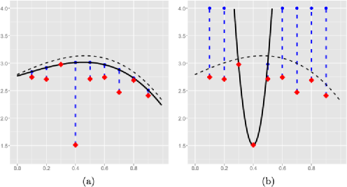
Figure 1: Dashed line: true function; solid line: estimated function; red squares: sample points; estimation point: fourth sample point from the left.

The adaptation problem consists of finding an (asymptotically) optimal bandwidth $h_{k}$ when neither the regression function $f$ nor the specific boundary behavior of the errors $(\varepsilon_{j})$ is known, which leads to different convergence rates. We follow the method inaugurated by Lepski lepski1990 and consider geometrically growing bandwidths with $h_{0}=n^{\mathfrak{h}_{0}-1}$, $\mathfrak{h}_{0}\in(0,1)$ and

$${h}_{k} = {h}_{0}\rho^{k},\qquad k=0,\ldots,K+1$$

$$\eqntext{\mbox{where }\rho>1\mbox{ and }K=\bigl{\lfloor}\log_{\rho}\bigl{(}n^{1-\mathfrak{h}_{0}}\bigr{)}\bigr{\rfloor}.}$$ (8)

The purely data-driven estimator $\hat{f}:=\tilde{f}_{\hat{k}}$ is defined as

$$\hat{k}:=\inf\bigl{\{}k=0,\ldots,K|\exists l\leq k\dvtx\|\tilde{f}_{k+1}-\tilde{f}_{l}\|>\hat{\mathfrak{z}}_{l}^{T}+\hat{\mathfrak{z}}_{k+1}^{T}\bigr{\}}\wedge K.$$ (9)

The critical values $\hat{\mathfrak{z}}_{l}^{T}$, $l=0,\ldots,K+1$ depend on the observations $\{Y_{i}\}_{1\leq i\leq n}$, and will be specified below. The basic idea is to increase the bandwidth $h_{k}$ as long as the distance (in some suitable seminorm $\|\cdot\|$) between the estimators is not significantly larger than the usual stochastic fluctuations of the estimators such that at $\hat{k}$ the bias is not yet dominating. In order to choose $\hat{\mathfrak{z}}_{l}^{T}$, the extreme-value index $\mathfrak{a}_{x}$, $\mathfrak{b}_{x}$ and the constant $\mathfrak{c}_{x}$ from equations (3) and (4) have to be estimated locally. For that purpose a quasi-negative-Hill method is developed in Section 3.2.

3 Asymptotic upper bounds

In this section we will study the convergence rate of our estimator $\hat{f}=\tilde{f}_{\hat{k}}$ with $\hat{k}$ as defined in (9) when the sample size $n$ tends to infinity. We will consider both the pointwise risk $\mathbb{E}_{f}|\hat{f}(x)-f(x)|^{2}$ for some fixed $x\in[0,1]$ and the $L_{q}$-risk $\mathbb{E}_{f}\int_{0}^{1}|\hat{f}(x)-f(x)|^{q}\,dx$ for $q\geq 1$. To deal with the upper bounds, first some preparatory remarks and work are necessary. Throughout this section, we suppose:

Assumption 3.1.

(i) $\mathfrak{c}_{x},\mathfrak{b}_{x},\mathfrak{a}_{x}\in H_{[0,1]}(\beta_{0},L_{0})$, where $\beta_{0},L_{0}>0$ and $\inf_{x\in[0,1]}\mathfrak{a}_{x},\mathfrak{c}_{x}>0$,

(ii) $\max_{1\leq j\leq n}\mathbb{E}[|\varepsilon_{j}|]<\infty$,

(iii) $(\varepsilon_{j})$ are independent, and the distribution of $\varepsilon_{j}$ satisfies (3), (4).

For our theoretical treatment, an important quantity in the sequel is the approximative tail-function

$$A_{x}(y)=-\mathfrak{c}_{x}y^{-1/\mathfrak{a}_{x}}\log(y)^{\mathfrak{b}_{x}},$$ (10)

since it asymptotically describes the quantile $\mathcal{U}_{x}(y)$.

3.1 General upper bounds

Most of our analysis relies on Theorem 3.1 and Proposition 3.1 below. These give rise to a decomposition, where the error for the implicitly defined base estimators $\tilde{f}_{k}(x)$ in (6) is split into a deterministic and a stochastic error part. Even though $\tilde{f}_{k}(x)$ is highly nonlinear, we obtain a relatively sharp and particularly simple upper bound.

Theorem 3.1

For any $x\in[0,1]$ and $\beta_{x}\in(0,\beta^{*}+1]$ there exist constants $c(\beta^{*},L_{x})$, $c(\beta^{*})$ and $J(\beta^{*})$, only depending on $\beta^{*}$ and $L_{x}$, respectively, such that

$$\bigl{|}\tilde{f}_{k}(x)-f(x)\bigr{|}$$

$$\qquad\leq c\bigl{(}\beta^{*},L\bigr{)}h_{k}^{\beta_{x}}$$

$$\quad\qquad{}+c\bigl{(}\beta^{*}\bigr{)}\max\bigl{\{}\bigl{|}Z_{j}(h_{k},x)\bigr{|}\dvtx j=1,\ldots,2J\bigl{(}\beta^{*}\bigr{)},x+h_{k}{\mathcal{I}}_{j}\subseteq[0,1]\bigr{\}}$$

holds true for all $f\in H_{\mathcal{N}(x)}(\beta,L)$ where

$$Z_{j}(h_{k},x) := \max\{\varepsilon_{i}\dvtx x_{i}\in x+h_{k}{\mathcal{I}}_{j}\}\quad\mbox{and}$$

$${\mathcal{I}}_{j} := \bigl{[}-1+(j-1)/J\bigl{(}\beta^{*}\bigr{)},-1+j/J\bigl{(}\beta^{*}\bigr{)}\bigr{]}.$$

Remark 1.

Interestingly, this decomposition holds true for any underlying distribution function $F$ and dependence structure within $(\varepsilon_{j})$. Its proof is entirely based on nonprobabilistic arguments and has an interesting connection to algebra. A generalization to arbitrary dimensions or other basis functions than polynomials seems challenging.

We continue the range of the indices $j$ of the $(x_{j},\varepsilon_{j})$ from $\{1,\ldots,n\}$ to $\mathbb{Z}$ while the equidistant location of the $x_{j}$ and the independence of the $\varepsilon_{j}$ is maintained. Then, Theorem 3.1 yields that with $c^{*}=c(\beta^{*},L)$

$$\bigl{|}\tilde{f}_{k}(x)-f(x)\bigr{|} \leq c^{*}h_{k}^{\beta_{x}}+c\bigl{(}\beta^{*}\bigr{)}\max\bigl{\{}\bigl{|}Z_{j}(h_{k},x)\bigr{|}\dvtx j=1,\ldots,2J\bigl{(}\beta^{*}\bigr{)}\bigr{\}},$$ (11)

$$\|\tilde{f}_{k}-f\|_{q} \leq c^{*}h_{k}^{\beta_{x}}+c\bigl{(}\beta^{*}\bigr{)}\bigl{\|}\max\bigl{\{}\bigl{|}Z_{j}(h_{k},\cdot)\bigr{|}\dvtx j=1,\ldots,2J\bigl{(}\beta^{*}\bigr{)}\bigr{\}}\bigr{\|}_{q},$$ (12)

where $\|\cdot\|_{q}$ denotes the $L_{q}([0,1])$-norm, $q\geq 1$. To pursue adaptivity, suppose that in terms of some seminorm $\|\cdot\|$, we can bound the error via

$$\|\tilde{f}_{k}-f\|\leq{R}_{k}+B_{k}\qquad\forall k=0,\ldots,K+1,f\in H_{\mathcal{N}(x)}(\beta,L),$$ (13)

for some nonnegative random variables $B_{k},R_{k}$, where $B_{k}$ increases in $k$ and ${R}_{k}$ decreases in $k$. Neither the $B_{k}$ nor the ${R}_{k}$ depend on $f$, only on $\beta_{x}$ and $L_{x}$. In the sequel $B_{k}$ will be a bias upper bound while ${R}_{k}$ is a bound on the stochastic error, which here—in contrast to usual mean regression—decays in $k$ for each noise realisation. The following fundamental proposition addresses both, the pointwise and the $L_{q}$-risk of the adaptive estimator, since the pointwise distance of function values at some $x$ as well as the $L_{q}$-distance of functions on $[0,1]$ define seminorms for $q\geq 1$.

Proposition 3.1

Let $\|\cdot\|$ denote some seminorm, and let $\tilde{f}_{k}$, $f$ lie in the corresponding normed space. Assume (13) and that the $\hat{\mathfrak{z}}_{k}^{T}$ decrease a.s. in $k$. Defining the oracle-type index

$$\hat{k}^{*}:=\inf\bigl{\{}k=0,\ldots,K-1\dvtx B_{k+1}>\hat{\mathfrak{z}}_{k+1}^{T}/2\bigr{\}}\wedge K,$$ (14)

we obtain for $q\geq 1$: [(a)]

$\displaystyle\mathbb{E}_{f}\bigl{[}\|\hat{f}-\tilde{f}_{\hat{k}^{*}}\|^{q}\mathbf{1}\bigl{(}\hat{k}>\hat{k}^{*}\bigr{)}\bigr{]}^{1/q}\leq\mathbb{E}_{f}\bigl{[}\bigl{(}\hat{\mathfrak{z}}_{\hat{k}^{*}}^{T}\bigr{)}^{q}\bigr{]}$,

$\displaystyle\mathbb{E}_{f}\bigl{[}\|\hat{f}-\tilde{f}_{\hat{k}^{*}}\|^{q}\mathbf{1}\bigl{(}\hat{k}<\hat{k}^{*}\bigr{)}\bigr{]}^{1/q}$
$\displaystyle\hskip 30.0pt\qquad\leq 2^{(2q-1)/q}\mathbb{E}_{f}\bigl{[}\hat{\mathfrak{z}}_{\hat{k}^{*}}^{q}\bigr{]}^{1/q}$
$\displaystyle\hskip 30.0pt\quad\qquad{}+2^{(2q-1)/q}\sum_{k=0}^{K-1}\mathbb{E}_{f}\bigl{[}{R}_{k}^{q}\mathbf{1}\bigl{(}\exists l\leq k\dvtx{R}_{l}>\hat{\mathfrak{z}}_{l}^{T}/2\bigr{)}\bigr{]}^{1/q}$.

3.2 Critical values and their estimation

Our adaptive procedure and particularly the question of optimality crucially hinge on the (estimated) critical values $\hat{\mathfrak{z}}_{k}^{T}$, and thereby as a quantile for the distribution function $F_{x}(-y^{-1})$ as $y\to\infty$. In the literature (de Haan and Ferreira dehaanbook2006 ), the standard, nonparametric quantile estimator is constructed via the approximation

$$\mathcal{U}_{x}(ty)\approx\mathcal{U}_{x}(y)+a_{x}(t)\bigl{(}y^{-1/\mathfrak{a}_{x}}-1\bigr{)}\mathfrak{a}_{x}\qquad\mbox{as }t,y\to\infty,$$ (15)

where the function $a_{x}(t)$ is a so-called first-order scale function. Unfortunately, this approach fails in our setup. The reason for this failure is the severely shifted sample $(Y_{j})$ (we do not observe $\varepsilon_{j}$) and the particular type of interpolation used in (15), which leads to an insufficient rate of convergence in the above approach. The bias that is induced by the shift will be present in any estimation method. This fact makes us believe that under model (1), quantile estimation for general regular varying distributions is not possible. Since for any $t>0$ we have the relation

$$F_{x}\bigl{(}A_{x}(n/t)\bigr{)}^{n}\bigl{(}1+\mbox{\scriptsize$\mathcal{O}$}(1)\bigr{)} = F_{x}\bigl{(}\mathcal{U}_{x}(n/t)\bigr{)}^{n}$$

$$= (1-t/n)^{n}$$

$$= e^{-t}\bigl{(}1+\mbox{\scriptsize$\mathcal{O}$}(1)\bigr{)}\qquad\mbox{as }n\to\infty,$$

a viable alternative is provided by a plug-in estimator $\widehat{A}_{x}(y)$, based on suitable estimates $\hat{\mathfrak{a}}_{x}$, $\hat{\mathfrak{b}}_{x}$ and $\hat{\mathfrak{c}}_{x}$. Here, the shift may be overcome by location invariant estimators for these quantities. The fact that these parameters additionally vary in $x$ with unknown smoothness degree adds another level of complexity and needs to be dealt with in a localized, adaptive manner. At this stage, it is worth mentioning that our adaptive procedure does not hinge on any particular type of quantile estimator. As a matter of fact, we only require the following property of an admissible quantile estimator $\widehat{A}_{x}(y)$.

Definition 1.

Given $x\in[0,1]$, let $\mathcal{Y}_{x}=[\log n,n^{4/\mathfrak{a}_{x}}]$ and $s\in\{0,1\}$. We call $\widehat{A}_{x}(y)$ admissible if for any fixed $v\in\mathbb{N}$ and constants $c_{1}^{-}<1<c_{1}^{+}$, which may be arbitrarily close to one, we have

$$P_{f}\biggl{(}c_{1}^{-}\leq\sup_{y\in\mathcal{Y}_{x}}\biggl{|}\frac{\widehat{A}_{x}^{(s)}(y)}{A_{x}^{(s)}(y)}\biggr{|}\leq c_{1}^{+}\biggr{)}=1-\mathcal{O}\bigl{(}n^{-v}\bigr{)},$$

uniformly over $f\in H_{\mathcal{N}(x)}(\beta,L)$, where $g^{(s)}(\cdot)$ denotes the $s$th derivative of a function $g(\cdot)$.

Remark 2.

Admissibility for $s=1$ is only required in case of the $L_{q}$-norm loss.

Now we shall construct an admissible estimator under Assumption 3.1. Even though the class of potential estimators seems to be quite large under Assumption 3.1, verifying the conditions of Definition 1 leads to quite technical and tedious calculations. Moreover, the requirement of location invariance rules out many prominent estimators from the literature. Regarding the shape parameter $\mathfrak{a}_{x}$, this eliminates, for instance, Hill-type estimators as possible candidates; see Alves fraga2002 and de Haan and Ferreira dehaanbook2006 . Possible alternatives are Pickand’s estimator (cf. Pickand pickandsIII1975 and Drees drees1995 ) or the probability weighted moment estimator by Hosking and Wallis hoskins1987 . These may, however, exhibit a poor performance in practice; see, for instance, de Haan and Peng dehaanpeng1998 for a comparison. In falk1995 , Falk proposed the negative Hill estimator, which, unlike to its positive counter part, is also location invariant; see also de Haan and Ferreira dehaanbook2006 . Transferring this approach to our setup, we construct estimators $\hat{\mathfrak{a}}_{x}$, $\hat{\mathfrak{b}}_{x}$ and $\hat{\mathfrak{c}}_{x}$ that are location invariant, and also inherit the favorable variance property of Hill’s estimator. Based on these estimates, we can use the plug-in estimator

$$\widehat{A}_{x}(y)=-\hat{\mathfrak{c}}_{x}(\log y)^{\hat{\mathfrak{b}}_{x}}y^{-1/\hat{\mathfrak{a}}_{x}}.$$ (17)

To construct the estimators $\hat{\mathfrak{a}}_{x}$, $\hat{\mathfrak{b}}_{x}$ and $\hat{\mathfrak{c}}_{x}$ for fixed $x\in[0,1]$, consider the neighborhoods $\mathcal{N}_{k}(x)=\{y\dvtx|x-y|\leq h_{k}\}$ for $k=0,\ldots,K-1$. Introduce the sets $\mathcal{S}_{k}(x)=\{Y_{i}\dvtx i/n\in\mathcal{N}_{k}(x)\}$, and note that its cardinality $\bar{n}_{k}(x):=\#\mathcal{S}_{k}(x)$ satisfies $nh_{k}\leq\bar{n}_{k}(x)\leq 2nh_{k}+1$. Let us rearrange the sample in $\mathcal{S}_{k}(x)$ as

$$Y_{1,\bar{n}_{k}(x)},Y_{2,\bar{n}_{k}(x)},\ldots,Y_{\bar{n}_{k}(x),\bar{n}_{k}(x)},$$ (18)

where $Y_{j,\bar{n}_{k}(x)}$ denotes the $j$th largest $Y_{i}\in\mathcal{S}_{k}(x)$. For each $k=0,\ldots,K-1$, let $m_{k}=m(\bar{n}_{k}(x))$ such that $m_{k}/\bar{n}_{k}\to 0$, where $\bar{n}_{k}=\bar{n}_{k}(x)$ to lighten the notation. In the literature, a common parametrization of $m_{k}$ is $m_{k}={\bar{n}_{k}}^{\mathfrak{m}}$ for $0<\mathfrak{m}\leq 1$. Before discussing the important issue of possible choices of $\mathfrak{m}$, we formally introduce our estimation procedure. Apart from the necessary location invariance, an estimator of ${A}_{x}(y)$ should also adapt to the unknown smoothness degree of the parameters ${\mathfrak{a}}_{x}$, ${\mathfrak{b}}_{x}$ and ${\mathfrak{c}}_{x}$. A related issue is dealt with in the literature; see, for instance, Drees drees2001 or Grama and Spokoiny gramaspokoiny2008 . In order to achieve this adaptivity, we apply a Lepski-type procedure to select among appropriate base estimators. We first tackle the problem of estimating ${\mathfrak{a}}_{x}$. Using Falk’s idea in falk1995 , we define

$$\qquad\frac{1}{\hat{\mathfrak{a}}_{x}(m_{k})}=\frac{1}{m_{k}}\sum_{i=2}^{m_{k}-1}\log\biggl{(}\frac{Y_{m_{k},\bar{n}_{k}}-Y_{1,\bar{n}_{k}}}{Y_{i,\bar{n}_{k}}-Y_{1,\bar{n}_{k}}}\biggr{)},\qquad k=0,1,\ldots,K-1.$$ (19)

Note that this estimator is clearly location invariant. For $\rho>1$ select the index $\hat{k}_{\mathfrak{a}}(x)$ via

$$\hat{k}_{\mathfrak{a}}(x) := \inf\bigl{\{}k=0,\ldots,K-1|\exists l\leq k\dvtx$$

$$\phantom{\inf\bigl{\{}}\bigl{|}\hat{\mathfrak{a}}_{x}^{-1}(m_{k+1})-\hat{\mathfrak{a}}_{x}^{-1}(m_{l})\bigr{|}>\rho^{-k}(\log n)^{-1}\bigr{\}}\wedge K.$$

As a final estimator, we put

$$\hat{\mathfrak{a}}_{x}^{-1}=\hat{\mathfrak{a}}_{x}^{-1}(m_{\hat{k}_{\mathfrak{a}}})\qquad\mbox{where }\hat{k}_{\mathfrak{a}}=\hat{k}_{\mathfrak{a}}(x).$$ (21)

For the estimation of ${\mathfrak{b}}_{x}$, we proceed in a similar manner. For $k=0,1,\ldots,K-1$, we put

$$\hat{\mathfrak{b}}_{x}(m_{k})=\frac{1}{m_{k}\log\log\bar{n}_{k}}\sum_{i=2}^{m_{k}-1}\log\biggl{(}\frac{Y_{i,\bar{n}_{k}}-Y_{1,\bar{n}_{k}}}{(\bar{n}_{k}/i)^{-1/\hat{\mathfrak{a}}_{x}(m_{k})}-(\bar{n}_{k}/1)^{-1/\hat{\mathfrak{a}}_{x}(m_{k})}}\biggr{)},$$ (22)

and select the index $\hat{k}_{\mathfrak{b}}(x)$ via

$$\hat{k}_{\mathfrak{b}}(x) := \inf\bigl{\{}k=0,\ldots,\hat{k}_{\mathfrak{a}}(x)|\exists l\leq k\dvtx$$

$$\hphantom{\inf\bigl{\{}}\bigl{|}\hat{\mathfrak{b}}_{x}(m_{k+1})-\hat{\mathfrak{b}}_{x}(m_{l})\bigr{|}>\rho^{-k}(\log\log n)^{-1}\bigr{\}}\wedge K.$$

As final estimator, we then put

$$\hat{\mathfrak{b}}_{x}=\hat{\mathfrak{b}}_{x}(m_{\hat{k}_{\mathfrak{b}}})\qquad\mbox{where }\hat{k}_{\mathfrak{b}}=\hat{k}_{\mathfrak{b}}(x).$$ (24)

Interestingly, it turns out that $\hat{\mathfrak{b}}_{x}=\mathfrak{b}_{x}+\frac{\log\mathfrak{c}_{x}}{\log\log nh_{\hat{k}_{\mathfrak{b}}}}(1+\mbox{\scriptsize$\mathcal{O}$}_{P}(1))$. Since this implies that

$$(\log nh_{k})^{\hat{\mathfrak{b}}_{x}} = \mathfrak{c}_{x}(\log nh_{k})^{\mathfrak{b}_{x}}\bigl{(}1+\mbox{\scriptsize$\mathcal{O}$}_{P}(1)\bigr{)}\qquad\mbox{for }k=0,\ldots,K-1,$$

there is no need to specifically estimate $\mathfrak{c}_{x}$, it is included in the bias for free. We are thus lead to the definition of our estimator

$$\widehat{A}_{x}(y)=-(\log y)^{\hat{\mathfrak{b}}_{x}}y^{-1/\hat{\mathfrak{a}}_{x}}.$$ (25)

For the consistent estimation of $\widehat{A}_{x}(\cdot)$, we need a relation between the initial bandwidth $h_{0}$ and the bias, induced by the parameter $\beta_{x}$. Note that such an assumption is inevitable, since any adaptive estimation procedure needs to start off with some initial bandwidth. Thus in the sequel, we will assume that

$$h_{0}^{\beta_{x}}\bigl{|}A_{x}(m_{0})\bigr{|}^{-1}=\mbox{\scriptsize$\mathcal{O}$}\bigl{(}(\log n)^{-1}\bigr{)}.$$ (26)

If $\mathfrak{h}_{0},\mathfrak{m}>0$ is such that

$$\mathfrak{m}\mathfrak{h}_{0}<(1-\mathfrak{h}_{0})\mathfrak{a}_{0}\beta_{0},$$ (27)

for some lower bounds

$$\mathfrak{a}_{0}\leq\mathfrak{a}_{x}\quad\mbox{and}\quad\beta_{0}\leq\beta_{x}$$ (28)

on the unknown parameters, then (26) is valid. In the supplementary material jirmeireisssuppl we prove the following result under the more general Assumption 10.1, which is implied by Assumption 3.1.

Proposition 3.2

Grant Assumption 10.1, and suppose that (26) is valid. Then $\widehat{A}_{x}(y)$ defined in (25) is admissible.

In practice the negative Hill estimator works well for $\mathfrak{a}_{x}\in(0,3/2]$ (and small $\mathfrak{b}_{x}$), but has increasing (asymptotically negligible) bias for $\mathfrak{a}_{x}>3/2$ and $\mathfrak{b}_{x}\neq 0$, which should be corrected in applications; see also Section 5, paragraph (B). Also note that our assumptions in Assumption 3.1 include cases where a CLT for an estimator $\hat{\mathfrak{a}}_{x}$ fails to hold, and only slower rates of convergence than $m_{k}^{-1/2}$ are possible. This is particularly the case if $\mathfrak{b}_{x}\neq 0$; we refer to de Haan and Ferreira dehaanbook2006 for details. In practice, the choice of the actual bandwidth $m_{k}$ (and hence $\mathfrak{m}$) is of significant relevance, and much research has been devoted to this subject; see, for instance, Drees Drees1998 and Drees et al. drees2001how . In fraga2002 , Alves addresses this question for a related (positive) location invariant Hill-type estimator both in theory (Theorem 2.2) and practice (concluding remarks and algorithm). Transferring the practical aspects, this amounts to the choice $m_{k}=2{\bar{n}_{k}}^{\mathfrak{m}}$, $\mathfrak{m}=2/3$ in our case. Still, any other choice also leads to the total optimal rates presented in Theorems 3.2 and 3.3, as long as $0<\mathfrak{m}<1$ holds.

3.3 Pointwise adaptation

Throughout this subsection we fix a point $x\in[0,1]$. For the seminorm in Proposition 3.1 we take $\|f\|:=|f(x)|$. According to Theorem 3.1, we set

$$B_{k} := c\bigl{(}\beta^{*},L\bigr{)}h_{k}^{\beta},$$

$${R}_{k} := c\bigl{(}\beta^{*}\bigr{)}\max\bigl{\{}\bigl{|}Z_{j}(h_{k},x)\bigr{|}\dvtx j=1,\ldots,2J\bigl{(}\beta^{*}\bigr{)}\bigr{\}},$$

in the notation of (13). The nonnegativity and monotonicity constraints on $B_{k}$ and $R_{k}$ are satisfied since $h_{k}$ increases. We define the oracle and estimated critical values as

$$\mathfrak{z}_{k}(x) = 4c\bigl{(}\beta^{*}\bigr{)}\biggl{|}A_{x}\biggl{(}\frac{\mathfrak{a}_{x}nh_{k}}{4J(\beta^{*})\log n}\biggr{)}\biggr{|},\qquad\hat{\mathfrak{z}}_{k}(x)=4c\bigl{(}\beta^{*}\bigr{)}\biggl{|}\widehat{A}_{x}\biggl{(}\frac{\hat{\mathfrak{a}}_{x}nh_{k}}{4J(\beta^{*})\log n}\biggr{)}\biggr{|},$$

for $k=0,\ldots,K-1$ and set ${\mathfrak{z}}_{K}(x)=\hat{\mathfrak{z}}_{K}(x):=0$. To lighten the notation, we often drop the index $x$ and write $\mathfrak{z}_{k}$ and $\hat{\mathfrak{z}}_{k}$. As outlined earlier in (3.2), this definition is motivated by the fact that $\mathcal{U}_{x}(y)\approx A_{x}(y)$ as $y\to\infty$. The critical values can thus be viewed as an appropriate estimate for certain extremal quantiles. The additional $\log n$-factor turns out to be the price to pay for adaption. We proceed by introducing the estimated truncated critical values as

$$\hat{\mathfrak{z}}_{k}^{T}=\min\{\hat{\mathfrak{z}}_{k},1\}.$$ (30)

The truncation of the estimator $\hat{\mathfrak{z}}_{k}^{T}$ is required to exclude a possible pathological behavior both in theory and practice. Note that this does not affect its proximity to $\mathfrak{z}_{k}$ if $\hat{\mathfrak{z}}_{k}$ is consistent, since $\mathfrak{z}_{k}\to 0$ uniformly in $k=0,\ldots,K-1$. We have the following pointwise result.

Theorem 3.2

Fix $x\in[0,1]$, and suppose $\mathfrak{a}_{x},\mathfrak{b}_{x},\mathfrak{c}_{x}$ and $\beta_{x}\in(0,\beta^{*}+1]$ are unknown with $\mathfrak{h}_{0}<\beta_{x}\mathfrak{a}_{x}/(\beta_{x}\mathfrak{a}_{x}+1)$. If Assumption 3.1 holds, then

$$\sup_{f\in H_{\mathcal{N}(x)}(\beta,L)}\mathbb{E}_{f}\bigl{[}\bigl{(}\hat{f}(x)-f(x)\bigr{)}^{2}\bigr{]}$$

$$\qquad=\mathcal{O}\bigl{(}(n/\log n)^{(-2\beta_{x})/(\mathfrak{a}_{x}\beta_{x}+1)}(\log n)^{(2\mathfrak{a}_{x}\mathfrak{b}_{x}\beta_{x})/(\mathfrak{a}_{x}\beta_{x}+1)}\bigr{)}.$$

As will be demonstrated in Section 4, this result is optimal in the minimax sense.

3.4 $L_{q}$-adaptation

Let us consider the $L_{q}([0,1])$-norm as seminorm in Proposition 3.1. Due to (12) we can choose

$$B_{k} := c\bigl{(}\beta^{*},L\bigr{)}h_{k}^{\beta},$$ (31)

$$R_{k} := c\bigl{(}\beta^{*}\bigr{)}\bigl{\|}\max\bigl{\{}\bigl{|}Z_{j}(h_{k},\cdot)\bigr{|}\dvtx j=1,\ldots,2J\bigl{(}\beta^{*}\bigr{)}\bigr{\}}\bigr{\|}_{q}$$ (32)

in the notation of (13). We verify that the nonnegativity and monotonicity constraints on $B_{k}$ and $R_{k}$ are satisfied for $\rho>1$ in (2) since for any $x\in[0,1]$ each interval $x+h_{k}{\mathcal{I}}_{j}$, $j=1,\ldots,2J(\beta^{*})$ is included in $x+h_{k+1}{\mathcal{I}}_{j^{\prime}}$ for some $j^{\prime}=1,\ldots,2J(\beta^{*})$ for any $k$. Throughout this paragraph, we assume that the parameters $\mathfrak{a}_{x},\mathfrak{b}_{x},\mathfrak{c}_{x}$ remain constant for $x\in[0,1]$. We denote these with $\mathfrak{a}_{F},\mathfrak{b}_{F},\mathfrak{c}_{F}$, and the corresponding $A_{x}(\cdot)$ with $A_{F}(\cdot)$.

The construction of the critical values is more intricate compared to the pointwise case, and relies on the following quantity. Introduce

$$\qquad\widehat{\mathit{IU}}_{n}(s,q)=\biggl{(}\int_{n^{-2/\hat{\mathfrak{a}}_{F}}}^{n^{1/2}}\bigl{(}(-\widehat{A}_{F})^{q}(s/y)\bigr{)}^{(1)}\exp(-y)\,dy\biggr{)}^{1/q},\qquad q\geq 1,$$ (33)

and the corresponding version ${\mathit{IU}}_{n}(s,q)$ where we replace $\widehat{A}_{F}(\cdot)$ by ${A}_{F}(\cdot)$ and $\hat{\mathfrak{a}}_{F}$ by $\mathfrak{a}_{F}$ [recall that $g^{(s)}(\cdot)$ denotes the $s$th derivative of a function $g(\cdot)$]. For $k=0,\ldots,K-1$, we introduce the critical values as

$$\mathfrak{z}_{k} = \sqrt{5}c\bigl{(}\beta^{*}\bigr{)}\biggl{|}{\mathit{IU}}_{n}\biggl{(}\frac{nh_{k}}{6J(\beta^{*})},q\biggr{)}\biggr{|},\qquad\hat{\mathfrak{z}}_{k}=\sqrt{5}c\bigl{(}\beta^{*}\bigr{)}\biggl{|}\widehat{\mathit{IU}}_{n}\biggl{(}\frac{nh_{k}}{6J(\beta^{*})},q\biggr{)}\biggr{|},$$

and set ${\mathfrak{z}}_{K}=\hat{\mathfrak{z}}_{K}:=0$. Moreover, we define the corresponding truncated values as

$$\hat{\mathfrak{z}}_{k}^{T}=\min\{\hat{\mathfrak{z}}_{k},1\}.$$ (34)

Unlike the pointwise case, the critical values do not correspond to an extremal quantile, but they can be considered as an estimate of $\mathbb{E}[R_{k}^{q}]^{1/q}$. This already indicates that the $L_{q}$-case is substantially different from the pointwise situation, and indeed additional, more refined arguments are necessary to prove the result given below.

Theorem 3.3

Suppose $\mathfrak{a}_{F}>0$ and $\beta\in(0,\beta^{*}+1]$ are unknown with $\beta\mathfrak{a}_{F}/(\beta\mathfrak{a}_{F}+1)>\mathfrak{h}_{0}$. We select $\rho\in\mathbb{N}$ with $\rho>1$. If $q\geq 1$, then the adaptive estimator $\hat{f}$ from Section 2 satisfies

$$\sup_{f\in H_{[0,1]}(\beta,L)}\mathbb{E}_{f}\bigl{[}\|\hat{f}-f\|_{q}^{q}\bigr{]}=\mathcal{O}\bigl{(}n^{(-q\beta)/(\mathfrak{a}_{F}\beta_{+}1)}(\log n)^{(q\beta\mathfrak{a}_{F}\mathfrak{b}_{F})/(\mathfrak{a}_{F}\beta_{+}1)}\bigr{)}.$$

Remark 3.

If one allows for $\mathfrak{a}_{x},\mathfrak{b}_{x},\mathfrak{c}_{x}\in H(\beta_{0},L)$ for $x\in[0,1]$, the above result remains valid if one takes the supremum over the above bound. This result is also optimal in the minimax sense.

Theorem 3.3 shows that the estimator $\hat{f}$ is $L_{q}$-adaptive; that is, it attains the minimax rates, which are optimal in the oracle setting of known $\mathfrak{a}_{F}$ and $\beta$, although it does not use these constants in its construction; see Theorem 4.2 below for the lower bound.

4 Asymptotic lower bounds

We show that the logarithmic loss in the convergence rate in Theorem 3.2 is unavoidable with respect to any estimator sequence of $f$. First, we treat the case $\mathfrak{a}_{x}\in(0,2]$ for which we derive a lower bound, even for a known error distribution. It suffices to treat the case where $\mathfrak{a}=\mathfrak{a}_{x}$, $\mathfrak{b}=\mathfrak{b}_{x}$ and $\mathfrak{c}=\mathfrak{c}_{x}$ remain constant for $x\in[0,1]$. We maintain this convention throughout this section.

We assume that the $\varepsilon_{j}$ have a Lebesgue density $f_{\varepsilon}$ which is continuous and strictly positive on $(-\infty,0)$, and vanishes on $[0,\infty]$. Moreover, we impose that the $\chi^{2}$-distance for the parametric location problem satisfies

$$\qquad\int_{-\infty}^{0}\bigl{|}f_{\varepsilon}(x+\vartheta)-f_{\varepsilon}(x)\bigr{|}^{2}/f_{\varepsilon}(x)\,dx\leq c_{\varepsilon}\vartheta^{\mathfrak{a}}|\log\vartheta|^{-\mathfrak{a}\mathfrak{b}}\qquad\forall\vartheta\in(0,1),$$ (35)

for some $\mathfrak{a}\in(0,2]$ and $\mathfrak{b}\in\mathbb{R}$. Note that $\mathfrak{a}$ and $\mathfrak{b}$ correspond to $\mathfrak{a}_{x}$ and $\mathfrak{b}_{x}$, respectively, in (3) and (4) with uniform $x$. As examples for such error densities with $\mathfrak{b}=0$, we consider the reflected gamma-densities

$$f_{\lambda}(x):=\frac{1}{\Gamma(\lambda)}(-x)^{\lambda-1}\exp(x){\mathbf{1}}_{(-\infty,0)}(x),\qquad x\in\mathbb{R},$$

for $\lambda\in[1,2)$. Thus, by $|(1+\vartheta/x)^{\lambda-1}-1|\leq\vartheta/|x|$ for $x\leq-\vartheta$ we have

$$\int_{-\infty}^{0}\bigl{|}f_{\lambda}(x+\vartheta)-f_{\lambda}(x)\bigr{|}^{2}/f_{\lambda}(x)\,dx$$

$$\qquad=\int_{-\infty}^{-\vartheta}\biggl{|}\biggl{(}1+\frac{\vartheta}{x}\biggr{)}^{\lambda-1}\exp(\vartheta)-1\biggr{|}^{2}f_{\lambda}(x)\,dx+\int_{-\vartheta}^{0}f_{\lambda}(x)\,dx$$

$$\qquad\leq 2\bigl{(}\exp(\vartheta)-1\bigr{)}^{2}+2\exp(2\vartheta)\vartheta^{2}$$

$$\quad\qquad{}+2\exp(2\vartheta)\vartheta^{2}\int_{-1}^{-\vartheta}x^{-2}f_{\lambda}(x)\,dx+\int_{-\vartheta}^{0}f_{\lambda}(x)\,dx$$

$$\qquad\leq\mathcal{O}\bigl{(}\vartheta^{2}\bigr{)}+\frac{2}{(2-\lambda)\Gamma(\lambda)}\exp(2\vartheta)\vartheta^{\lambda}\bigl{(}1-\vartheta^{2-\lambda}\bigr{)}+\vartheta^{\lambda}/\Gamma(\lambda+1)$$

$$\qquad=\mathcal{O}\bigl{(}\vartheta^{\lambda}\bigr{)}.$$

Therefore, the reflected gamma-density satisfies (35) when putting $\mathfrak{a}=\lambda$. Note that (35) implies (3), (4) under the Assumption 3.1(i). The following theorem together with the upper bound in Theorem 3.2 shows that pointwise adaptation causes a logarithmic loss in the convergence rates, which is known from regular regression when inserting $\mathfrak{a}=2$.

Theorem 4.1

Assume condition (35), and fix some arbitrary $x_{0}\in[0,1]$, $\beta_{1}>\beta_{2}>0$ and $C_{0},C_{1}>0$. Let $\{\hat{f}_{n}(x_{0})\}_{n}$ be any sequence of estimators of $f(x_{0})$ based on the data $Y_{1},\ldots,Y_{n}$ which satisfies

$$\sup_{f\in{\mathcal{H}}_{[0,1]}(\beta_{1},C_{0})}\mathbb{E}_{f}\bigl{|}\hat{f}_{n}(x_{0})-f(x_{0})\bigr{|}^{2}=\mathcal{O}\bigl{(}n^{-2\beta_{2}/(1+\beta_{2}\mathfrak{a})}n^{-\xi}\bigr{)},$$

for some $\xi>0$. Then this estimator sequence suffers from the lower bound

$$\liminf_{n\to\infty}(n/\log n)^{(2\beta_{2})/(1+\mathfrak{a}\beta_{2})}(\log n)^{(-2\mathfrak{a}\mathfrak{b}\beta_{2})/(1+\mathfrak{a}\beta_{2})}$$

$$\qquad{}\times\sup_{f\in{\mathcal{H}}_{[0,1]}(\beta_{2},C_{1})}\mathbb{E}_{f}\bigl{|}\hat{f}_{n}(x_{0})-f(x_{0})\bigr{|}^{2}>0.$$

For completeness we also derive the $L_{q}$-minimax optimality of the convergence rates established by our estimator $\hat{f}$ in Theorem 3.3. This rectifies a conjecture after Theorem 3 in Hall and van Keilegom hallkeilegom2009 for general smoothness degrees.

Theorem 4.2

Assume condition (35), and let $\{\hat{f}_{n}\}_{n}$ be any sequence of estimators of $f$ based on the data $Y_{1},\ldots,Y_{n}$. Then, for any fixed $q\geq 1$, we have

$$\liminf_{n\to\infty}n^{\beta_{2}/(1+\mathfrak{a}\beta_{2})}(\log n)^{(-\mathfrak{a}\mathfrak{b}\beta_{2})/(1+\mathfrak{a}\beta_{2})}\sup_{f\in{\mathcal{H}}_{[0,1]}(\beta_{2},C_{1})}\mathbb{E}_{f}\bigl{[}\|\hat{f}_{n}-f\|_{q}\bigr{]}>0.$$

Now we focus on the case $\mathfrak{a}>2$. To simplify some of the technical arguments in the proofs, we restrict to the case $\mathfrak{b}=0$. If $\mathfrak{a}>2$, the convergence rates become slower than in the Gaussian case. Instead of the convenient conditions (3) and (4), we choose the slightly different Definition 2, under which the upper bound proofs obviously still hold true.

Definition 2.

Let $\mathfrak{a}>2$, $0<\mathfrak{h}_{0}\leq 1$, and denote with ${\mathcal{D}}_{n}(\mathfrak{a},\mathfrak{h}_{0})$ the set of all error distribution functions whose quantile functions $\mathcal{U}^{(n)}$ satisfy: [(ii)]

$\displaystyle\sup_{y\in(0,\infty]}\biggl{|}\frac{\mathcal{U}^{(n)}(y)}{A(y/2)}\biggr{|}\leq 1\qquad\mbox{where }A(y)=-y^{-1/\mathfrak{a}}$,

$\displaystyle\sup_{n}\sup_{y\in[\log N,N]}\biggl{|}\frac{\mathcal{U}^{(n)}(y)}{A(y)}-1\biggr{|}|\log y|\leq(\log n)^{-2},\qquad N=n^{\mathfrak{h}_{0}}$. Note that we have ${\mathcal{D}}_{n}(\mathfrak{a},\mathfrak{h}_{0})\subseteq{\mathcal{D}}_{n}(\mathfrak{a},\mathfrak{h}_{0}^{\prime})$ if $\mathfrak{h}_{0}>\mathfrak{h}_{0}^{\prime}$.

The above conditions particularly imply that the distribution function $F(y)=F^{(n)}(y)$ [or likewise $\mathcal{U}(y)=\mathcal{U}^{(n)}(y)$] of the errors $\varepsilon_{j}$ may depend on $n$. While the lower bound results for $\mathfrak{a}\leq 2$ still hold true if the error distribution is known and independent of the design point, here two competing types of regression errors have to be considered in the proof. Note that the probability measure thus depends on both the regression function $f$ and the distribution function $F$, which we mark as $P_{f,F}$.

Theorem 4.3

Fix some arbitrary $x_{0}\in[0,1]$, $\beta_{1}>\beta_{2}>0$ and $C_{0},C_{1}>0$. Let $\mathfrak{a}>2$, and suppose that $\mathfrak{h}_{0}<\frac{\beta_{2}}{\mathfrak{a}\beta_{2}+1}$. Let $\{\hat{f}_{n}(x_{0})\}_{n}$ be any sequence of estimators of $f(x_{0})$ based on the data $Y_{1},\ldots,Y_{n}$ which satisfies

$$\sup_{f\in{\mathcal{H}}_{[0,1]}(\beta_{1},C_{0})}\sup_{F\in{\mathcal{D}}_{n}(\mathfrak{a},\mathfrak{h}_{0})}\mathbb{E}_{f,F}\bigl{|}\hat{f}_{n}(x_{0})-f(x_{0})\bigr{|}^{2}=\mathcal{O}\bigl{(}n^{-2\beta_{2}/(1+\mathfrak{a}\beta_{2})}n^{-\xi}\bigr{)},$$

for some $\xi>0$. Then this estimator sequence suffers from the lower bound

$$\liminf_{n\to\infty}(n/\log n)^{(2\beta_{2})/(1+\mathfrak{a}\beta_{2})}\sup_{f\in{\mathcal{H}}_{[0,1]}(\beta_{2},C_{1})}\sup_{F\in{\mathcal{D}}_{n}(\mathfrak{a},\mathfrak{h}_{0})}\mathbb{E}_{f,F}\bigl{|}\hat{f}_{n}(x_{0})-f(x_{0})\bigr{|}^{2}>0.$$

The proofs of Theorems 4.1, 4.2 and 4.3 are given in the supplementary material jirmeireisssuppl . Theorem 4.2 can be extended in a similar way to $\mathfrak{a}>2$, a detailed proof is omitted.

5 Numerical simulations and real data application

The aim of this section is to highlight some of the theoretical findings with numerical examples. We will briefly touch on the following points:

[(A)]

Performance of the estimator on different function types and the corresponding effect on adaptive bandwidth selection.

The effect of different parameters $\mathfrak{a}_{x}$, $\mathfrak{b}_{x}$ and $\mathfrak{c}_{x}$.

Application: wolf sunspot-number.

Application: yearly best men’s outdoor 1500 times.

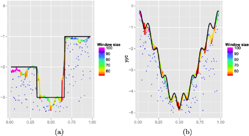
Figure 2: (a) Function $f=f_{1}$, $\beta^{*}=2$, $n=200$, $\varepsilon_{j}\sim\operatorname{exp}(1)$; (b) function $f=f_{2}$, $\beta^{*}=2$, $n=200$, $\varepsilon_{j}\sim\operatorname{exp}(1)$.

In order to illustrate the behavior of the estimation procedure, we consider three different regression functions, displayed in black in Figures 2 and 3(a),

$$f_{1}(x) = -2\cdot\mathbf{1}(x<1/3)-3\cdot\mathbf{1}(1/3\leq x<2/3)-\mathbf{1}(2/3<x),\qquad x\in[0,1],$$

$$f_{2}(x) = -2+2\cos(2\pi x)+0.3\sin(19\pi x),\qquad x\in[0,1].$$

They are similar to those discussed in Chichignoud chichi2012 . Comments on the implementation and setup are given in the supplementary material jirmeireisssuppl , together with a numerical comparison to oracle estimators and additional simulations. All of the results can be reproduced by R-code, available at jirmeireissrcode .

[(A)]

Figure 2 gives a first impression on the behavior and accuracy of our estimation procedure. In both cases, the errors $\varepsilon_{j}$ follow an exponential distribution $\operatorname{exp}(1)$, and the sample size is $n=200$. The window size in Figure 2 corresponds to the local sample size, chosen by the adaptive procedure. Even though $n$ is only of moderate size, the estimation procedure achieves good results by essentially recovering the shape of the underlying regression, also in the wiggly case of function $f_{2}$. Simulations of other nonparametric (adaptive) estimators that do not take the nonregularity into account (cf. Lepski and Spokoiny lepskispokoiny1997 and the R-packages crs, gam, smooth-spline, etc.) often fail to do so (with mean correction).

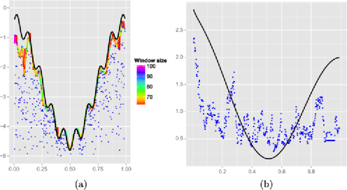
Figure 3: (a) Function $f=f_{2}$, $\beta^{*}=4$, $n=600$, $\varepsilon_{j}\sim\Gamma(\mathfrak{a}_{x},1)$; (b) $\mathfrak{a}_{x}$ (black line) and $\hat{\mathfrak{a}}_{x}$ (blue points).

The effect of the shape (type) of the function on the bandwidth selection is highlighted by a color-scheme, ranging from dark red (low) to dark violet (high). In order to understand the “coloring of the estimator,” one has to recall that the estimation procedure always tries to fit a local polynomial which “stays above the observations.” At first sight, this can lead to a surprisingly large bandwidth selection at particular spots. The bandwidth size is not necessarily an indicator for estimation accuracy. The reason for this effect is the maximum function: additional observations are taken into account as long as this does not substantially change the maximum, which can lead to a surprisingly large bandwidth selection. [(B)]

Here, the setup is different from paragraph (A). We consider a sample size of $n=600$, and we let the parameters vary in $x$. The impact of $\mathfrak{b}_{x}$, $\mathfrak{c}_{x}$ (and their estimates) is rather insignificant on the total estimator. This is not unexpected and can be explained by the very definition in (10). We therefore focus only on the parameter $\mathfrak{a}_{x}$ in this paragraph. We consider the setup where the errors follow a Gamma distribution $\varepsilon_{j}\sim\Gamma(\mathfrak{a}_{x},1)$ and $\mathfrak{a}_{x}$ varies according to the function $\mathfrak{a}_{x}=\sin(2\pi x+\pi/2)-\sqrt{(}1-(x-1)^{2})+2$. We only discuss function $f_{2}$ here; a more comprehensive comparison including an additional function $f_{3}$ is given in the supplementary material jirmeireisssuppl . As can be clearly seen in Figure 3, there is a considerable increase in estimation accuracy as $\mathfrak{a}_{x}$ gets closer to zero. Generally speaking, for larger $\mathfrak{a}_{x}$ the bias can be pronounced, and this is indeed the case at the left top of Figure 3(a). It simply turns out that there are no observations at all near the regression function $f_{2}$, which leads to the large gap. An approximate bias correction [e.g., by $\widehat{\mathit{IU}}(nh_{k},1)$, Section 3.4] could be applied, but we do not pursue this any further. Figure 3 also reveals that the estimator $\hat{\mathfrak{a}}_{x}$ (blue) has a large variance and problems with quickly oscillating regression functions $f$ (compare with the supplementary material jirmeireisssuppl ). On the other hand, it seems to capture the general trend of decrease and increase to some extent. We would like to point out, however, that these estimations are very sample dependent, and due to the relatively small, local sample size, the actual behavior of local samples may deviate significantly from a large sample of $\Gamma(\mathfrak{a}_{x},1)$-distributed random variables. Significant overestimation leads to critical values that are too large, which in turn results in a slight overestimation of the regression function; see the very center of Figure 3(a) ($0.4$ to $0.6$). The opposite effect can be observed at both endpoints of Figure 3(a), where an underestimation is present, which leads to critical values that are too small. Also note that the negative Hill estimator generally tends to underestimate $\mathfrak{a}_{x}$ if $\mathfrak{a}_{x}\geq 3/2$, which is due to an (asymptotic negligible) bias; cf. de Haan and Ferreira dehaanbook2006 . A thorough bias correction requires a precise second order asymptotic expansion of the limit distribution of the negative Hill estimator, which is beyond the scope of this paper. Note, however, that a rudimentary bias correction is available in our implemented code. Another, more practical option would be to consider the estimation of $\mathfrak{a}_{x}$ itself as a regression problem with one-sided errors, treating the local estimates $\hat{\mathfrak{a}}_{x}$ as “sample.”

A similar behavior appears when considering function $f_{1}$, but, as can be expected, the estimates $\hat{\mathfrak{a}}_{x}$ are more accurate. [(C)]

The Wolf sunspot number (often also referred to as Zürich number), is a measure for the number of sunspots and groups of sunspots present on the surface of the sun. Initiated by Rudolf Wolf in 1848 in Zürich, this famous time series has been studied for decades by physicists, astronomers and statisticians. The relative sunspot number $R_{t}$ is computed via the formula

$$R_{t}=K_{t}(10g_{t}+s_{t}),$$ (36)

where $s_{t}$ is the number of individual spots observed at time $t$, $g_{t}$ is the number of groups observed at time $t$ and $K_{t}$ is the observatory factor or personal reduction coefficient. The factor $K_{t}$ (always positive and usually smaller than one) depends on the individual observatories around the world and is intended to convert the data to Wolf’s original scale, but also to correct for seeing conditions and other diversions. In general, we have the relationship

$$\mbox{observed data}=\mbox{observed fraction}\times\mbox{true value},$$ (37)

where we always have that the random variable $\mbox{observed fraction}\in(0,1]$. Therefore, the factor $K_{t}$ can be viewed as an aggregated individual estimate for the right scaling. Over the last century, many different models have been fit to the sunspot data; we refer to He heli2001 and Solanki et al. Solanki20041084 for an overview. In particular, the study of the sunspots has attracted people long before 1848. Recorded observations are, for instance, due to Thomas Harriot, Johannes and David Fabricius (in the 17th century), Edward Maunder and many more. However, much uncertainty lies in these data, and the sunspot time series before 1850 is usually referred to as “unreliable” or “poor.” It is therefore interesting to reconstruct the “true time series” or at least reduce some uncertainty. We attempt do so for the period from 1749 to 1810, based on monthly observations. Let us reconsider model (36). Given $R_{t}$, we may then postulate the model

$$R_{t}=X_{t}\mathcal{S}\bigl{(}10g_{t}^{\circ}+s_{t}^{\circ}\bigr{)},$$ (38)

where $g_{t}^{\circ}$, $s_{t}^{\circ}$ denote the corresponding true sunspot values, and $X_{t}\in(0,1]$. This means we concentrate all random components in $X_{t}$, which is in spirit of model (37). We point out that this is only one possible way from a modeling perspective; we refer to Kneip et al. kneip2012 or Koenker et al. koenker1994 and the references therein for alternatives and more general models. In our setup, the parameter $\mathcal{S}>0$ reflects the support of the “misjudgment” of the observer. For example, $\mathcal{S}\leq 1$ is equivalent with the assumption that every observer always reports less than the true value. As we see below, it incorporates the systematic bias of the observers. By using a $\log$-transformation, we have the additive model

$$\log R_{t}=\log X_{t}+\log\bigl{(}10g_{t}^{\circ}+s_{t}^{\circ}\bigr{)}+\log\mathcal{S},$$ (39)

which can be interpreted as a nonparametric regression problem with stochastic error $\log X_{t}\in(-\infty,0]$. The goal is to estimate the function $f(t)=\log(10g_{t}^{\circ}+s_{t}^{\circ})$, the “true” relative sunspot number. Such estimation results can serve as input to structural physical models for sunspot activity like the time series approaches mentioned above. Unfortunately, one can only estimate $f(t)+\log\mathcal{S}$, where the bias $\log\mathcal{S}$ cannot be removed without any further assumptions. This is clear from the nonidentifiability in model (38). Generally $\mathcal{S}$ is a systematic (intrinsic) bias, which has to be overcome using other sources of information (expert judgement). Any other statistical approach will also suffer from such a global bias.

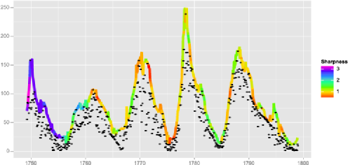
Figure 4: Estimated Wolf number with $\mathcal{S}=1$, $\beta^{*}=5$.

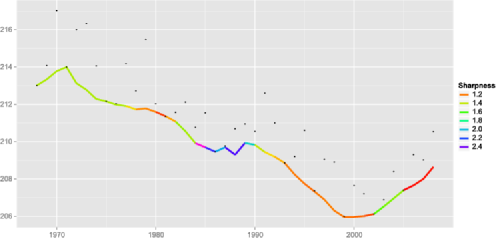
Figure 5: Yearly best men’s outdoor 1500 m times in seconds with estimated boundary ($\beta^{*}=2$).

The results of the estimated sunspot number is given in Figure 4, where we plotted an estimate corresponding to $\mathcal{S}=1$. Given that observation techniques where much less advanced and coordinated in the 18th and 19th centuries, it is reasonable to assume $\mathcal{S}\leq 1$. Apart from the estimated sunspot number itself, our estimation procedure provides a map from the uncertainty level $\mathcal{S}$ to the true sunspot number $f(t)$. The sharpness $\mathfrak{a}_{x}$ seems to mainly vary within the interval $[0,3.5]$. Finally, we would like to comment on the “peaks” around $1768$ and $1774$. These peaks are artifacts and originate from a too large initial bandwith selection at these particular points. However, for the sake of reproducibility, we have kept them and did not make any ad-hoc, data-dependent changes.

[(D)]

As another example we discuss the yearly best men’s outdoor 1500 m times starting from 1966, depicted in Figure 5 with estimated lower boundary. Following Knight knight2006 , the boundary can be interpreted as the best possible time for a given year. This data set displays an interesting behavior. As can be clearly seen from Figure 5, the boundary steadily decreases from 1970 until around the year 2000, followed by a sudden and sharp increase. This event leaves room for speculation. Let us mention that until the year 2000, it had been very difficult to distinguish between the biological and synthetical EPO. The breakthrough was achieved by Lasne and Ceaurriz lasneceaurriz2000 , and since then, more and more refined and efficient doping tests have been developed. It seems plausible that this change and advance in doping controls has lead to the sudden increase, but it might as well be attributed to some other reason.

6 Proof of the main results

Throughout the proofs, we make the following convention. For two sequences of positive numbers $a_{n}$ and $b_{n}$, we write $a_{n}\gtrsim b_{n}$ when $a_{n}\geq Cb_{n}$ for some absolute constant $C>0$, and $a_{n}\lesssim b_{n}$ when $b_{n}\gtrsim a_{n}$. Finally, we write $a_{n}\thicksim b_{n}$ when both $a_{n}\lesssim b_{n}$ and $a_{n}\gtrsim b_{n}$ hold.

Proof of Theorem 3.1 Throughout the proof, we fix some arbitrary $x\in[0,1]$ and write $\beta=\beta_{x}$ to lighten the notation. The data $Y_{i}$, $i=1,\ldots,n$, can be written as

$$Y_{i}=\sum_{j=0}^{\beta^{*}}b_{j}(x_{i}-x)^{j}+\varepsilon_{i}+\Delta_{i},$$

where $\Delta_{i}:=f(x_{i})-\sum_{j=0}^{\beta^{*}}b_{j}(x_{i}-x)^{j}$. Putting $\Delta:=\max\{|\Delta_{i}|\dvtx|x_{i}-x|\leq h_{k}\}$, the coefficients $b_{j}$ are chosen as the Taylor coefficients $b_{j}=f^{(j)}(x)/j!$ for $j\leq\langle\beta\rangle$ and $b_{j}=0$ otherwise, such that by the Hölder condition on $f^{(\langle\beta\rangle)}$ in the Taylor remainder term

$$\Delta\leq Lh_{k}^{\beta}/\bigl{(}\langle\beta\rangle+1\bigr{)}!.$$ (40)

Selecting $b_{0}^{*}:=b_{0}+\Delta$, $b_{j}^{*}:=b_{j}$, $j>0$, we realize that

$$\sum_{j=0}^{\beta^{*}}b_{j}^{*}(x_{i}-x)^{j} = \sum_{j=0}^{\beta^{*}}b_{j}(x_{i}-x)^{j}+\Delta\geq Y_{i}$$

$$\eqntext{\forall i=1,\ldots,n\mbox{ with }|x-x_{i}|\leq h_{k},}$$ (41)

so that by the definition of the $\hat{b}_{j}$, $j=0,\ldots,\beta^{*}$, we have

$$\sum_{|x_{i}-x|\leq h_{k}}\sum_{j=0}^{\beta^{*}}\hat{b}_{j}(x_{i}-x)^{j} \leq \sum_{|x_{i}-x|\leq h_{k}}\sum_{j=0}^{\beta^{*}}b_{j}^{*}(x_{i}-x)^{j}$$

$$= \sum_{|x_{i}-x|\leq h_{k}}\Biggl{\{}\sum_{j=0}^{\beta^{*}}b_{j}(x_{i}-x)^{j}+\Delta\Biggr{\}}.$$

We define the polynomial

$$Q(y):=\sum_{j=0}^{\beta^{*}}(\hat{b}_{j}-b_{j})(y-x)^{j}-\Delta.$$

Then inequality (6) implies that

$$\inf_{n,k,f}\int Q(y)\,d\lambda_{n}(y)\leq 0,$$ (43)

where $\lambda_{n}$ denotes the uniform probability measure on the discrete set $\{x_{i}\dvtx|x_{i}-x|\leq h_{k}\}$ inside the interval $[x-h_{k},x+h_{k}]\cap[0,1]$. We introduce the sets $Q^{\pm}$ of all $y\in[x-h_{k},x+h_{k}]\cap[0,1]$ such that $Q(y)$ is nonnegative or negative, respectively. Our first task is to show that

$$\inf_{n,k,f}\lambda_{n}\bigl{(}Q^{-}\bigr{)}>0\quad\mbox{or}\quad Q=0\qquad\mbox{identically}.$$ (44)

In the latter case Theorem 3.1 is trivially true; hence we focus on the case where $Q\neq 0$. As $Q^{-}$ is the complement of $Q^{+}$ with respect to $[x-h_{k},x+h_{k}]\cap[0,1]$, we have $\lambda_{n}(Q^{+})\geq 1/2$ or $\lambda_{n}(Q^{-})\geq 1/2$. Clearly, we have (44) in the second case, so let us study the situation where $\lambda_{n}(Q^{+})\geq 1/2$.

As $Q$ is a polynomial with degree $\leq\beta^{*}$ the set $Q^{+}$ equals the union of at most $\beta^{*}+1$ disjoint sub-intervals of $[x-h_{k},x+h_{k}]\cap[0,1]$. The number of all design points in $[x-h_{k},x+h_{k}]$ is denoted by $m_{k}$. Hence, there exists at least one interval $I_{0}^{+}\subseteq Q^{+}$ such that $\lambda_{n}(I_{0}^{+})\geq 1/(2\beta^{*}+2)$. At least $\lceil m_{k}/(2\beta^{*}+2)\rceil$ of the $x_{i}$ lie in $I_{0}^{+}$ so that, due to the equidistant location of the design points, the length of $I_{0}^{+}$ is larger or equal to

$$\bigl{\{}\bigl{\lceil}m_{k}/\bigl{(}2\beta^{*}+2\bigr{)}\bigr{\rceil}-1\bigr{\}}/n\geq\bigl{\{}\bigl{\lceil}\lfloor nh_{k}\rfloor/\bigl{(}2\beta^{*}+2\bigr{)}\bigr{\rceil}-1\bigr{\}}/n\geq c_{1}\bigl{(}\beta^{*}\bigr{)}\cdot h_{k},$$

for $n$ sufficiently large and some uniform constant $c_{1}(\beta^{*})>0$ which does not depend on $n$ or $k$, but only on $\beta^{*}$. The polynomial $Q$ takes only nonnegative values on the interval $I_{0}^{+}$. By Lemma 6.1 below there exists some interval $I_{1}^{+}\subseteq I_{0}^{+}$ with the length $c_{2}(\beta^{*})h_{k}$ such that

$$\inf_{y\in I_{1}^{+}}\bigl{|}Q(y)\bigr{|}\geq c_{3}\bigl{(}\beta^{*}\bigr{)}\cdot\sup_{|z-x|\leq h_{k}}\bigl{|}Q(z)\bigr{|},$$

where the constants $c_{2}(\beta^{*}),c_{3}(\beta^{*})>0$ only depend on $\beta^{*}$. It follows from there that

$$\int_{Q^{+}}Q(y)\,d\lambda_{n}(y) \geq \int_{I_{1}^{+}}Q(y)\,d\lambda_{n}(y)$$

$$\geq \lambda_{n}\bigl{(}I_{1}^{+}\bigr{)}\cdot\inf_{y\in I_{1}^{+}}\bigl{|}Q(y)\bigr{|}$$

$$\geq \lambda_{n}\bigl{(}I_{1}^{+}\bigr{)}c_{3}\bigl{(}\beta^{*}\bigr{)}\cdot\sup_{|z-x|\leq h_{k}}\bigl{|}Q(z)\bigr{|}.$$

On the other hand we learn from (43) that

$$\int_{Q^{+}}Q(y)\,d\lambda_{n}(y)\leq\int_{Q^{-}}\bigl{|}Q(y)\bigr{|}\,d\lambda_{n}(y)\leq\lambda_{n}\bigl{(}Q^{-}\bigr{)}\cdot\sup_{|z-x|\leq h_{k}}\bigl{|}Q(z)\bigr{|},$$

so that

$$\lambda_{n}\bigl{(}Q^{-}\bigr{)} \geq \lambda_{n}\bigl{(}I_{1}^{+}\bigr{)}c_{3}\bigl{(}\beta^{*}\bigr{)}\geq c_{3}\bigl{(}\beta^{*}\bigr{)}\cdot\bigl{(}c_{2}\bigl{(}\beta^{*}\bigr{)}h_{k}n-1\bigr{)}/m_{k}$$

$$\geq c_{3}\bigl{(}\beta^{*}\bigr{)}\cdot\bigl{(}c_{2}\bigl{(}\beta^{*}\bigr{)}-n^{-\mathfrak{h}_{0}}\bigr{)}/\bigl{(}2+n^{-\mathfrak{h}_{0}}\bigr{)},$$

unless $Q=0$ identically. Thus (44) has been shown.

Using the arguments as above, we can now find some interval $I_{0}^{-}\subseteq Q^{-}$ whose length is bounded from below by a constant (only depending on $\beta^{*}$) times $h_{k}$. By Lemma 6.1 there exists an interval $I_{1}^{-}\subseteq I_{0}^{-}$, whose length is also bounded from below by a constant (only depending on $\beta^{*}$) times $h_{k}$ and on which $|Q|$ is bounded from below by a uniform multiple of

$$\sup_{|z-x|\leq h_{k}}\bigl{|}Q(z)\bigr{|}\geq\bigl{|}Q(x)\bigr{|}\geq|\hat{b}_{0}-b_{0}|-\Delta.$$

This implies that

$$\inf_{y\in I_{1}^{-}}\bigl{(}-Q(y)\bigr{)}\geq c_{4}\bigl{(}\beta^{*}\bigr{)}\bigl{(}|\hat{b}_{0}-b_{0}|-\Delta\bigr{)}.$$ (45)

On the other hand, for all $x_{i}\in I_{1}^{-}$ we have

$$Q(x_{i}) = \sum_{j=0}^{\beta^{*}}\hat{b}_{j}(x_{i}-x)^{j}+\Delta_{i}-f(x_{i})-\Delta\geq Y_{i}-f(x_{i})-2\Delta.$$ (46)

Combining the inequalities in (45) and (46), we conclude that

$$\bigl{|}\tilde{f}_{k}(x)-f(x)\bigr{|}=|\hat{b}_{0}-b_{0}|\leq-c^{*}\bigl{(}\beta^{*}\bigr{)}\max\bigl{\{}\varepsilon_{i}\dvtx x_{i}\in I_{1}^{-}\bigr{\}}+c^{*}\bigl{(}\beta^{*}\bigr{)}\Delta$$

for some positive constant $c^{*}(\beta^{*})$. Choosing $J(\beta^{*})$ sufficiently large (regardless of $k$, $n$ and $f$) there exists some $l=1,\ldots,2J(\beta^{*})$ such that $x+h_{k}{\mathcal{I}}_{l}\subseteq I_{1}^{-}$, and hence

$$\bigl{|}\tilde{f}_{k}(x)-f(x)\bigr{|}\leq c^{*}\bigl{(}\beta^{*}\bigr{)}\Delta-c^{*}\bigl{(}\beta^{*}\bigr{)}\cdot Z_{j}(h_{k},x),$$

which completes the proof.

Lemma 6.1

Let $Q$ by any polynomial with the degree $\leq\beta^{*}$ and $I\subseteq[x-h_{k},x+h_{k}]$ be an interval with the length $\geq c_{5}(\beta^{*})h_{k}$ for some constant $c_{5}(\beta^{*})>0$. Then there exist some finite constants $c_{6}(\beta^{*}),c_{7}(\beta^{*})>0$ which only depend on $\beta^{*}$ and some interval $I^{*}\subseteq I$ with the length $\geq c_{6}(\beta^{*})h_{k}$ such that

$$\inf_{y\in I^{*}}\bigl{|}Q(y)\bigr{|}\geq c_{7}\bigl{(}\beta^{*}\bigr{)}\cdot\sup_{|z-x|\leq h_{k}}\bigl{|}Q(z)\bigr{|}.$$

If $Q$ is a constant function, the assertion is satisfied by putting $c=1$. Otherwise, by the fundamental theorem of algebra, $Q$ can be represented by

$$Q(y)=\alpha_{Q}\prod_{j=1}^{\beta^{\prime}}(y-y_{j}),$$

where $1\leq\beta^{\prime}\leq\beta^{*}$, the $y_{j}$ denote the complex-valued roots of $Q$. By the pigeon hole principle there exists some square $I_{1}^{+}\times[-c_{5}(\beta^{*})h_{k}/(2\beta^{*}+2),\break c_{5}(\beta^{*})h_{k}/(2\beta^{*}+2)]$ in the complex plane which does not contain any $y_{j}$ where $I_{1}^{+}\subseteq I$ has the length $c_{5}(\beta^{*})h_{k}/(\beta^{*}+1)$. Now we shrink that square by the factor $1/2$ where the center of the square does not change, leading to the square $I_{2}^{+}\times[-c_{5}(\beta^{*})h_{k}/(4\beta^{*}+4),c_{5}(\beta^{*})h_{k}/(4\beta^{*}+4)]$. Thus, for any $y$ in this shrinked square, the distance between $y$ and any $y_{j}$ is bounded from below by $c_{5}(\beta^{*})h_{k}/(4\beta^{*}+4)$ and by $|y_{j}-x|-h_{k}$. If the latter bound dominates, we have $|y_{j}-x|\geq\{1+c_{5}(\beta^{*})/(4\beta^{*}+4)\}\cdot h_{k}$. Then the distance between any $z\in[x-h_{k},x+h_{k}]$ and $y_{j}$ has the upper bound

$$|y_{j}-x|+h_{k}\leq|y_{j}-y|+2h_{k}\leq\bigl{\{}1+\bigl{(}8\beta^{*}+8\bigr{)}/c_{5}\bigl{(}\beta^{*}\bigr{)}\bigr{\}}\cdot|y_{j}-y|,$$

when applying the first bound. Otherwise, if the first bound dominates, we have

$$|z-y_{j}| \leq |y_{j}-x|+h_{k}\leq\bigl{\{}2+c_{5}\bigl{(}\beta^{*}\bigr{)}/\bigl{(}4\beta^{*}+4\bigr{)}\bigr{\}}\cdot h_{k}$$

$$\leq |y-y_{j}|\cdot\bigl{(}4\beta^{*}+4\bigr{)}\bigl{\{}2/c_{5}\bigl{(}\beta^{*}\bigr{)}+1/\bigl{(}4\beta^{*}+4\bigr{)}\bigr{\}}.$$

In both cases $|z-y_{j}|$ is bounded from above by a uniform constant $c_{6}(\beta^{*})$ times $|y-y_{j}|$. Then we learn from the root-decomposition of the polynomial $Q$ that

$$\inf_{y\in I^{*}}\bigl{|}Q(y)\bigr{|}\geq c_{7}\bigl{(}\beta^{*}\bigr{)}\cdot\sup_{|z-x|\leq h_{k}}\bigl{|}Q(z)\bigr{|},$$

for some deterministic constant $c_{7}(\beta^{*})>0$, which only depends on $\beta^{*}$.

Proof of Proposition 3.1 Part (a) follows directly from the definition of Lepski’s method. For part (b) we obtain from (13), and repeated application of the triangle and Jensen’s inequality that

$$\mathbb{E}_{f}\bigl{[}\|\hat{f}-\tilde{f}_{\hat{k}^{*}}\|^{q}\mathbf{1}\bigl{(}\hat{k}<\hat{k}^{*}\bigr{)}\bigr{]}^{1/q}$$

$$\qquad\leq\mathbb{E}_{f}\bigl{[}\|\tilde{f}_{\hat{k}}-f\|^{q}\mathbf{1}\bigl{(}\hat{k}<\hat{k}^{*}\bigr{)}\bigr{]}^{1/q}+\mathbb{E}_{f}\bigl{[}\|\tilde{f}_{\hat{k}^{*}}-f\|^{q}\mathbf{1}\bigl{(}\hat{k}<\hat{k}^{*}\bigr{)}\bigr{]}^{1/q}$$

$$\qquad\leq 2^{(q-2)/q}$$

$$\quad\qquad{}\times\bigl{(}\mathbb{E}_{f}\bigl{[}\bigl{(}{R}_{\hat{k}}^{q}+B_{\hat{k}}^{q}\bigr{)}\mathbf{1}\bigl{(}\hat{k}<\hat{k}^{*}\bigr{)}\bigr{]}^{1/q}+\mathbb{E}_{f}\bigl{[}\bigl{(}{R}_{\hat{k}^{*}}^{q}+B_{\hat{k}^{*}}^{q}\bigr{)}\mathbf{1}\bigl{(}\hat{k}<\hat{k}^{*}\bigr{)}\bigr{]}^{1/q}\bigr{)}$$

$$\qquad\leq 2^{(2q-1)/{q}}\bigl{(}\mathbb{E}_{f}\bigl{[}B_{\hat{k}^{*}}^{q}\bigr{]}^{1/q}+\mathbb{E}_{f}\bigl{[}{R}_{\hat{k}}^{q}\mathbf{1}\bigl{(}\hat{k}<\hat{k}^{*}\bigr{)}\bigr{]}^{1/q}\bigr{)}$$

$$\qquad\leq 2^{(2q-1)/q}\Biggl{(}\mathbb{E}_{f}\bigl{[}\hat{\mathfrak{z}}_{\hat{k}^{*}}^{q}\bigr{]}^{1/q}+\sum_{k=0}^{K-1}\mathbb{E}_{f}\bigl{[}{R}_{k}^{q}\mathbf{1}\bigl{(}\hat{k}=k,k<\hat{k}^{*}\bigr{)}\bigr{]}^{1/q}\Biggr{)},$$

where we also used that $R_{k}$ decreases in $k$ and $B_{k}$ increases in $k$. Note that

$$\mathbf{1}\bigl{(}\hat{k}=k,k<\hat{k}^{*}\bigr{)} \leq \mathbf{1}\bigl{(}\exists l\leq k\dvtx\|\tilde{f}_{k+1}-\tilde{f}_{l}\|>\hat{\mathfrak{z}}_{l}^{T}+\hat{\mathfrak{z}}_{k+1}^{T}\bigr{)}\cdot\mathbf{1}\bigl{(}k<\hat{k}^{*}\bigr{)}$$

$$\leq \mathbf{1}\bigl{(}\exists l\leq k\dvtx\|\tilde{f}_{k+1}-f\|+\|f-\tilde{f}_{l}\|>\hat{\mathfrak{z}}_{l}^{T}+\hat{\mathfrak{z}}_{k+1}^{T}\bigr{)}\cdot\mathbf{1}\bigl{(}k<\hat{k}^{*}\bigr{)}$$

$$\leq \mathbf{1}\bigl{(}\exists l\leq k\dvtx{R}_{l}+B_{k+1}>\hat{\mathfrak{z}}_{l}^{T}\bigr{)}\cdot\mathbf{1}\bigl{(}B_{k+1}\leq\hat{\mathfrak{z}}_{k+1}^{T}/2\bigr{)}$$

$$\leq \mathbf{1}\bigl{(}\exists l\leq k\dvtx{R}_{l}>\hat{\mathfrak{z}}_{l}^{T}/2\bigr{)}.$$

Inserting this inequality into (6) completes the proof.

In the sequel, the following three lemmas will be useful. The proofs are given in the supplementary material jirmeireisssuppl .

Lemma 6.2

If $y,t\to\infty$ and

$$y = \mathfrak{c}(\log t)^{\mathfrak{b}}t^{\mathfrak{a}}\bigl{(}1+\mbox{\scriptsize$\mathcal{O}$}(1)\bigr{)},\qquad\mathfrak{c},\mathfrak{a}>0,\mathfrak{b}\in\mathbb{R},$$

then

$$t = \bigl{(}\mathfrak{c}^{-1}\bigl{(}\log y^{1/\mathfrak{a}}\bigr{)}^{-\mathfrak{b}}y\bigr{)}^{1/\mathfrak{a}}+\mathcal{O}(1).$$

In particular, if we have $v=\mathcal{U}_{x}(y)$ with $v\to 0$, then

$$F_{x}(v) = 1-\mathfrak{c}_{x}^{-\mathfrak{a}_{x}}\bigl{(}\log|v|^{-1/\mathfrak{a}_{x}}\bigr{)}^{-\mathfrak{b}_{x}\mathfrak{a}_{x}}|v|^{\mathfrak{a}_{x}}\bigl{(}1+\mbox{\scriptsize$\mathcal{O}$}(1)\bigr{)}.$$

Lemma 6.3

For $1\leq j_{0},j_{1}\leq n$, let $\mathcal{J}=\{j_{0},\ldots,j_{1}\}$ such that $|j_{0}-j_{1}|/n=\mathcal{O}(n^{-\rho_{0}})$ for some $0<\rho_{0}<1$. If $u\to 0$, $u\leq-n^{-\rho_{1}}$ for some $\rho_{1}>0$, then

$$\prod_{j\in\mathcal{J}}P\bigl{(}\varepsilon_{j}\leq A_{x_{j_{0}}}\bigl{(}-u^{-1}\bigr{)}\bigr{)} \leq e^{\#\mathcal{J}c_{3}^{-}u},$$

where $c_{3}^{-}<1$ may be chosen arbitrarily close to one.

Lemma 6.4

Let $(q_{n})_{n}$ be a real-valued sequence which satisfies $q_{n}\in[1,\log n]$ for all integer $n$, and denote with $F(\cdot)$ the c.d.f. of $\varepsilon$. Then we have

$$\mathbb{E}\bigl{|}\max\{\varepsilon_{1},\ldots,\varepsilon_{n}\}\bigr{|}^{q_{n}}\leq\bigl{(}1+\mbox{ \scriptsize$\mathcal{O}$}(1)\bigr{)}\int_{0}^{n^{1/2}}\bigl{(}(-\mathcal{U})^{q_{n}}(n/y)\bigr{)}^{(1)}\exp(-y)\,dy.$$

If $\mathcal{U}(\cdot)$ is not differentiable, replace $\mathcal{U}(\cdot)$ with $c_{2}^{+}A(\cdot)$ in the above inequality, where $c_{2}^{+}>1$ can be chosen arbitrarily close to one. If $q_{n}=q$ is finite and independent of $n$, we obtain that

$$\mathbb{E}\bigl{|}\max\{\varepsilon_{1},\ldots,\varepsilon_{n}\}\bigr{|}^{q}=\mathcal{O}\bigl{(}(\log n)^{q\mathfrak{b}_{F}}n^{-q/\mathfrak{a}_{F}}\bigr{)}.$$

For arbitrary $q_{n}\in[1,\log n]$ we have

$$\mathcal{O}\bigl{(}n^{-c_{2}^{+}\mathfrak{a}_{F}/q_{n}}\bigr{)} \leq \int_{0}^{\infty}F\bigl{(}-x^{1/{q_{n}}}\bigr{)}^{n}\,dx\leq\mathcal{O}\bigl{(}n^{-c_{2}^{-}\mathfrak{a}_{F}/q_{n}}\bigr{)},$$

where $0<c_{2}^{-}<1<c_{2}^{+}$ can be chosen arbitrarily close to one.

Proof of Theorem 3.2 In the course of the proof we will frequently apply Proposition 3.2. We may do so since condition $\mathfrak{h}_{0}<\beta_{x}\mathfrak{a}_{x}/(\beta_{x}\mathfrak{a}_{x}+1)$ implies (27). The general strategy is the following. By the triangle inequality and Jensen’s inequality, we have

$$\quad\mathbb{E}_{f}\bigl{[}\bigl{(}\hat{f}(x)-f(x)\bigr{)}^{2}\bigr{]}\leq 2\mathbb{E}_{f}\bigl{[}\bigl{(}\hat{f}(x)-\tilde{f}_{\hat{k}^{*}}\bigr{)}^{2}\bigr{]}+2\mathbb{E}_{f}\bigl{[}\bigl{(}\tilde{f}_{\hat{k}^{*}}-f(x)\bigr{)}^{2}\bigr{]},$$ (48)

and we will treat both quantities separately. In order to deal with the first, Proposition 3.1 implies that it suffices to consider

$$\sup_{f\in H_{\mathcal{N}(x)}(\beta,L)}\mathbb{E}_{f}\bigl{[}\bigl{(}\hat{\mathfrak{z}}_{\hat{k}^{*}}^{T}\bigr{)}^{2}\bigr{]}^{1/2}+\sup_{f\in H_{\mathcal{N}(x)}(\beta,L)}\sum_{k=0}^{K-1}\mathbb{E}_{f}\bigl{[}{R}_{k}^{2}\mathbf{1}\bigl{(}\exists l\leq k\dvtx{R}_{l}>\hat{\mathfrak{z}}_{l}^{T}/2\bigr{)}\bigr{]}^{1/2}$$

$$\qquad=:I+\sum_{k=0}^{K-1}\mathit{II}_{k}.$$

To treat $I$, we require the following simple lemma; the proof is given in the supplementary material jirmeireisssuppl .

Lemma 6.5

Let $q\geq 1$. Under the assumptions of Theorem 3.2, we have uniformly over $f\in H_{\mathcal{N}(x)}(\beta,L)$

$$\mathbb{E}_{f}\bigl{[}\bigl{(}\hat{\mathfrak{z}}_{\hat{k}^{*}}^{T}\bigr{)}^{q}\bigr{]} \leq \bigl{(}c_{1}^{+}\bigr{)}^{q}\mathbb{E}_{f}\bigl{[}\bigl{(}\mathfrak{z}_{\hat{k}^{*}}^{T}\bigr{)}^{q}\bigr{]}+\mathcal{O}\bigl{(}n^{-q/\mathfrak{a}_{x}}\bigr{)},$$

where $c_{1}^{+}>1$.

Applying the above result with $q=2$ we obtain

$$I^{2}\leq\bigl{(}c_{1}^{+}\bigr{)}^{2}\mathbb{E}_{f}\bigl{[}\bigl{(}\mathfrak{z}_{\hat{k}^{*}}^{T}\bigr{)}^{2}\bigr{]}+\mathcal{O}\bigl{(}n^{-2/\mathfrak{a}_{x}}\bigr{)},$$ (49)

and it remains to deal with $\mathbb{E}_{f}[(\mathfrak{z}_{\hat{k}^{*}}^{T})^{2}]$. We define

$$k^{\pm}:=\inf\bigl{\{}k=0,\ldots,K-1\dvtx B_{k+1}>c_{2}^{\pm}\mathfrak{z}_{k+1}^{T}/2\bigr{\}}\wedge K.$$

On the event ${\mathcal{A}}_{n}=\{c_{2}^{-}\mathfrak{z}_{k}\leq\hat{\mathfrak{z}}_{k}\leq c_{2}^{+}\mathfrak{z}_{k}\mbox{ for all }k=0,\ldots,K-1\}$ we have $k^{-}\leq\hat{k}^{*}\leq k^{+}$. From Proposition 3.2 we infer $P(\mathcal{A}_{n}^{c})=\mathcal{O}(n^{-v}\log n)$ due to$K=\mathcal{O}(\log n)$. Since $\mathfrak{z}_{k}$ decreases monotonically in $k$, we deduce $\mathbb{E}[(\mathfrak{z}_{\hat{k}^{*}}^{T})^{2}]\leq\mathfrak{z}_{k^{-}}^{2}+\mathcal{O}(n^{-2/\mathfrak{a}_{x}})$. Note that the deterministic sequences $(h_{k}^{\pm})$ satisfy (see Lemma 6.2 for details)

$$\mathfrak{z}_{k^{-}} \thicksim -\bigl{(}h_{k}^{\pm}\bigr{)}^{\beta_{x}}\quad\mbox{and}$$

$$h_{k^{\pm}} \thicksim (n/\log n)^{-1/(\mathfrak{a}_{x}\beta_{x}+1)}(\log n)^{(\mathfrak{a}_{x}\mathfrak{b}_{x})/(\mathfrak{a}_{x}\beta_{x}+1)},$$

under our assumption $\mathfrak{h}_{0}<\beta_{0}\mathfrak{a}_{0}/(\beta_{0}\mathfrak{a}_{0}+1)$. We obtain

$$\sup_{f\in H_{\mathcal{N}(x)}(\beta,L)}\mathbb{E}_{f}\bigl{[}\bigl{(}\hat{\mathfrak{z}}{}^{T}_{\hat{k}^{*}}\bigr{)}^{2}\bigr{]}$$

(51)

$$\qquad=\mathcal{O}\bigl{(}(n/\log n)^{(-2\beta_{x})/(\mathfrak{a}_{x}\beta_{x}+1)}(\log n)^{(2\mathfrak{a}_{x}\mathfrak{b}_{x}\beta_{x})/(\mathfrak{a}_{x}\beta_{x}+1)}\bigr{)},$$

and it remains to deal with the second part. Let $\mathcal{B}_{k}=\{\exists l\leq k\dvtx{R}_{l}>\hat{\mathfrak{z}}_{l}^{T}/2\}$. Then for $\delta_{0}=n^{-\mathfrak{h}_{0}/\mathfrak{a}_{x}}$, we have

$$\mathit{II}_{k}^{2} = \int_{0}^{\infty}P_{f}\bigl{(}R_{k}^{2}\mathbf{1}(\mathcal{B}_{k})\geq x\bigr{)}\,dx\leq\int_{0}^{\delta_{0}}P_{f}(\mathcal{B}_{k})\,dx+\int_{\delta_{0}}^{\infty}P\bigl{(}R_{k}^{2}\geq x\bigr{)}\,dx$$

$$\leq \delta_{0}\sum_{l=0}^{k}P_{f}\bigl{(}{R}_{l}>\hat{\mathfrak{z}}_{l}^{T}/2\bigr{)}+\int_{\delta_{0}}^{\infty}P\bigl{(}R_{k}^{2}\geq x\bigr{)}\,dx=:\mathit{III}_{k}+\mathit{IV}_{k}.$$

We first deal with $\mathit{III}_{k}$. Recall that for $j=1,\ldots,2J(\beta^{*})$ we have

$$Z_{j}(h_{k},x)=\max\{\varepsilon_{i}\dvtx x_{i}\in x+h_{k}{\mathcal{I}}_{j}\}$$

and

$${\mathcal{I}}_{j}:=\bigl{[}-1+(j-1)/J\bigl{(}\beta^{*}\bigr{)},-1+j/J\bigl{(}\beta^{*}\bigr{)}\bigr{]}.$$

Put $\mathcal{J}_{j}(l)=\{0,1/n,2/n,\ldots,1\}\cap\{x+h_{l}{\mathcal{I}}_{j}\}$ for $j=1,\ldots,2J(\beta^{*})$, and note that $\#\mathcal{J}_{j}(l)\geq nh_{l}/2J(\beta^{*})$. An application of Proposition 3.2 and Theorem 3.1 then yields that

$$P_{f}\bigl{(}{R}_{l}>\hat{\mathfrak{z}}_{l}^{T}/2\bigr{)} \leq \sum_{j=1}^{J(\beta^{*})}P\bigl{(}\bigl{|}Z_{j}(h_{l},x)\bigr{|}>c_{1}^{-}\mathfrak{z}_{l}\bigr{)}+\mathcal{O}\bigl{(}n^{-2/\mathfrak{a}_{x}}\bigr{)}$$

$$\leq \sum_{j=1}^{2J(\beta^{*})}\prod_{i\in\mathcal{J}_{j}(l)}P\bigl{(}\varepsilon_{i}<-c_{1}^{-}\mathfrak{z}_{l}\bigr{)}+\mathcal{O}\bigl{(}n^{-2/\mathfrak{a}_{x}}\bigr{)},$$

where $c_{1}^{-}<1$ may be chosen arbitrarily close to one. Arguing as in Lemma 6.3 we obtain

$$\prod_{i\in\mathcal{J}_{j}}P\bigl{(}\varepsilon_{i}>-c_{1}^{-}\mathfrak{z}_{l}\bigr{)}=\mathcal{O}\bigl{(}n^{-2c_{2}^{-}/\mathfrak{a}_{x}}\bigr{)},$$ (53)

where $c_{2}^{-}<1$ may be chosen arbitrarily close to one. Hence we obtain that

$$\qquad\mathit{III}_{k}\leq\delta_{0}\sum_{l=0}^{k}\sum_{j=1}^{2J(\beta^{*})}\mathcal{O}\bigl{(}n^{-2c_{2}^{-}/\mathfrak{a}_{x}}\bigr{)}=\mathcal{O}\bigl{(}K\delta_{0}n^{-2c_{2}^{-}/\mathfrak{a}_{x}}\bigr{)}=\mathcal{O}\bigl{(}n^{-2/\mathfrak{a}_{x}}\bigr{)},$$ (54)

since $K=\mathcal{O}(\log n)$. For dealing with $\mathit{IV}_{k}$, set $\eta_{0}=\exp(n^{\mathfrak{h}_{0}/4})$. Let $u_{x}=A_{x}^{-1}(\delta_{0})$. Then Lemma 6.2 implies that $u_{x}<-n^{-\mathfrak{h}_{0}/2}$ for large enough $n$. Then as in (53), it follows from Lemma 6.3 that for sufficiently large $n$,

$$\int_{\delta_{0}}^{\eta_{k}}P\bigl{(}R_{k}^{2}\geq x\bigr{)}\,dx = \int_{\delta_{0}}^{\eta_{k}}P\bigl{(}R_{k}\leq-x^{1/2}\bigr{)}\,dx$$

$$\leq \eta_{k}\sum_{j=1}^{2J(\beta^{*})}\prod_{i\in\mathcal{J}_{j}(k)}P\bigl{(}\varepsilon_{i}<A_{x}\bigl{(}-n^{-\mathfrak{h}_{0}/2}\bigr{)}\bigr{)}$$

$$\leq \eta_{k}\sum_{j=1}^{2J(\beta^{*})}\exp\bigl{(}-\#\mathcal{J}_{j(k)}n^{-\mathfrak{h}_{0}/2}\bigr{)}$$

$$\leq \eta_{k}\sum_{j=1}^{2J(\beta^{*})}\exp\bigl{(}-n^{\mathfrak{h}_{0}/2}\bigr{)}=\mathcal{O}\bigl{(}\exp\bigl{(}-n^{\mathfrak{h}_{0}/4}\bigr{)}\bigr{)}.$$

Let $p>2$. Since $\mathbb{E}[|R_{k}|^{p}]=\mathcal{O}(1)$ by Lemma 6.4, it follows from the Markov inequality that

$$\int_{\eta_{k}}^{\infty}P\bigl{(}R_{k}^{2}\geq x\bigr{)}\,dx \leq \int_{\eta_{k}}^{\infty}x^{-p/2}\mathbb{E}\bigl{[}|R_{k}|^{p}\bigr{]}\,dx=\frac{2}{p-2}\eta_{k}^{-p/2+1}\mathcal{O}(1).$$

Combining the above and (54), it follows that $\mathit{IV}_{k}=\mathcal{O}(\exp(-n^{\mathfrak{h}_{0}/8}))$, which in turn yields

$$\mathit{II}_{k}^{2}=\mathit{III}_{k}+\mathit{IV}_{k}=\mathcal{O}\bigl{(}n^{-2/\mathfrak{a}_{x}}\bigr{)}+\mathcal{O}\bigl{(}\exp\bigl{(}-n^{\mathfrak{h}_{0}/8}\bigr{)}\bigr{)}=\mathcal{O}\bigl{(}n^{-2/\mathfrak{a}_{x}}\bigr{)}.$$ (55)

We thus conclude

$$\sum_{k=0}^{K-1}\mathit{II}_{k} = \mathcal{O}\bigl{(}Kn^{-1/\mathfrak{a}_{x}}\bigr{)}=\mathcal{O}\bigl{(}\log nn^{-1/\mathfrak{a}_{x}}\bigr{)}$$

$$= \mbox{\scriptsize$\mathcal{O}$}\bigl{(}(n\log n)^{-\beta_{x}/(\mathfrak{a}_{x}\beta_{x}+1)}(\log n)^{(\mathfrak{a}_{x}\mathfrak{b}_{x})/({\mathfrak{a}_{x}\beta_{x}+1})}\bigr{)}.$$

Piecing everything together and taking squares, we arrive at

$$\sup_{f\in H_{\mathcal{N}(x)}(\beta,L)}\mathbb{E}_{f}\bigl{[}\bigl{(}\hat{f}(x)-\tilde{f}_{\hat{k}^{*}}\bigr{)}^{2}\bigr{]}$$

(56)

$$\qquad=\mathcal{O}\bigl{(}(n\log n)^{-\beta_{x}/({\mathfrak{a}_{x}\beta_{x}+1})}(\log n)^{(\mathfrak{a}_{x}\mathfrak{b}_{x})/(\mathfrak{a}_{x}\beta_{x}+1)}\bigr{)}.$$

To complete the proof, it remains to deal with $\mathbb{E}_{f}[(\tilde{f}_{\hat{k}^{*}}-f(x))^{2}]$. Let $p^{\prime}>2$. Then by (3.3) and the triangle, Jensen and Hölder inequalities, we have

$$\mathbb{E}_{f}\bigl{[}\bigl{(}\hat{f}(x)-\tilde{f}_{\hat{k}^{*}}\bigr{)}^{2}\bigr{]} \leq 2\mathbb{E}_{f}\bigl{[}R_{\hat{k}^{*}}^{2}+B_{\hat{k}^{*}}^{2}\bigr{]}$$ (58)

$$\leq 2\mathbb{E}_{f}\bigl{[}R_{\hat{k}^{*}}^{2}\mathbf{1}(\mathcal{A}_{n})+B_{\hat{k}^{*}}^{2}\mathbf{1}(\mathcal{A}_{n})\bigr{]}$$

$${}+P\bigl{(}\mathcal{A}_{n}^{c}\bigr{)}^{(p^{\prime}-2)/p^{\prime}}\bigl{(}\mathbb{E}\bigl{[}R_{k^{-}}^{p^{\prime}}\bigr{]}^{1/p^{\prime}}+\mathcal{O}(L_{x})\bigr{)}.$$

Hence Proposition 3.2, Lemma 6.4 and (6) imply that the above is of order

$$\mathbb{E}_{f}\bigl{[}R_{\hat{k}^{*}}^{2}+B_{\hat{k}^{*}}^{2}\bigr{]} \leq 2\mathbb{E}_{f}\bigl{[}R_{{k}^{-}}^{2}\bigr{]}+B_{k^{+}}^{2}+\mathcal{O}\bigl{(}n^{-2/\mathfrak{a}_{x}}\bigr{)}$$

$$= \mathcal{O}\bigl{(}n_{k^{-}}^{-2/\mathfrak{a}_{x}}(\log n_{k^{-}})^{2\mathfrak{b}_{x}}+\mathfrak{z}_{k^{+}}^{2}+n^{-2/\mathfrak{a}_{x}}\bigr{)}$$

$$= \mathcal{O}\bigl{(}(n\log n)^{(-2\beta_{x})/(\mathfrak{a}_{x}\beta_{x}+1)}(\log n)^{(2\mathfrak{a}_{x}\mathfrak{b}_{x})/(\mathfrak{a}_{x}\beta_{x}+1)}\bigr{)}.$$

The above bound is uniform over $H_{\mathcal{N}(x)}(\beta,L)$, and the proof is complete.

Proof of Theorem 3.3 For the proof we require the following lemma, which provides a sub-polynomial upper bound on the probability that $R_{k}$ exceeds the threshold $\hat{\mathfrak{z}}_{l}^{T}/2$.

Lemma 6.6

Suppose $h_{k}\leq\exp(-c_{H}\log^{\gamma}n)$ for fixed constants $\gamma\in(0,1)$, $c_{H}>0$. Grant Assumption 3.1, and let $\mathfrak{m},\mathfrak{a}_{0},\beta_{0},\mathfrak{h}_{0}$ satisfy (27) in view of (28). Then

$$\sup_{k=0,\ldots,K-1}P\bigl{(}R_{k}>\hat{\mathfrak{z}}_{l}^{T}/2\bigr{)}=\mathcal{O}\bigl{(}\exp\bigl{(}-c_{H}\log^{1+\gamma}n/2q\bigr{)}\bigr{)},$$

as $n\to\infty$.

Let $p>q$. Then Lemma 6.4 gives

$$\mathbb{E}\bigl{[}R_{k}^{p}\bigr{]}^{q/p}=\mathcal{O}\bigl{(}(nh_{k})^{-q/\mathfrak{a}_{F}}(\log nh_{k})^{q\mathfrak{b}_{F}}\bigr{)}.$$ (60)

An application of Hölder’s inequality, (60) and Lemma 6.6 yields that

$$\sup_{f\in H_{[0,1]}(\beta,L)}\sum_{k=0}^{K-1}\mathbb{E}_{f}\bigl{[}{R}_{k}^{q}\mathbf{1}\bigl{(}\exists l\leq k\dvtx{R}_{l}>\hat{\mathfrak{z}}_{l}^{T}/2\bigr{)}\bigr{]}^{1/q}$$

$$\qquad\leq\sum_{k=0}^{K}(k+1)^{(p-q)/p}1_{[0,\exp(-c_{H}\log^{\gamma}n)]}(h_{k})$$

$$\hskip 45.0pt{}\times\mathcal{O}\bigl{(}n^{-\mathfrak{h}_{0}/\mathfrak{a}_{F}}\cdot\exp\bigl{(}-c_{H}/q(p-q)\log^{1+\gamma}n/[2qp]\bigr{)}\bigr{)}$$ (61)

$$\quad\qquad{}+\sum_{k=0}^{K}1_{(\exp(-c_{H}\log^{\gamma}n),\infty)}(h_{k})\cdot(nh_{k})^{-1/\mathfrak{a}_{F}}$$

$$\qquad=\mathcal{O}\bigl{(}n^{-c_{2}^{-}/\mathfrak{a}_{F}}\exp\bigl{(}[c_{H}/\mathfrak{a}_{F}]\log^{\gamma}n\bigr{)}\cdot\log n\bigr{)}.$$

Choosing $c_{H},\gamma>0$ sufficiently small, the above is of order $\mathcal{O}(n^{-c_{3}^{-}/\mathfrak{a}_{F}})$, where $c_{3}^{-}<1$ can be chosen arbitrarily close to one. According to Proposition 3.1 it remains to bound the expectation $\mathbb{E}_{f}[(\hat{\mathfrak{z}}{}^{T}_{\hat{k}^{*}})^{q}]$ uniformly over $f\in H_{[0,1]}(\beta,L)$. Applying Lemma 6.5, we obtain that uniformly over $f\in H_{[0,1]}(\beta,L)$

$$\mathbb{E}\bigl{[}\bigl{(}\hat{\mathfrak{z}}_{\hat{k}^{*}}^{T}\bigr{)}^{q}\bigr{]} \leq \bigl{(}Tc_{1}^{+}\bigr{)}^{q}\mathbb{E}_{f}\bigl{[}(\mathfrak{z}_{\hat{k}^{*}})^{q}\bigr{]}+\mathcal{O}\bigl{(}n^{-q/\mathfrak{a}_{F}}\bigr{)}.$$

To deal with $\mathbb{E}_{f}[(\mathfrak{z}_{\hat{k}^{*}})^{q}]$, we introduce

$$k^{\pm}:=\inf\bigl{\{}k=0,\ldots,K-1\dvtx B_{k+1}>c_{2}^{\pm}\mathfrak{z}_{k+1}^{T}/2\bigr{\}}\wedge K.$$

On the event $\mathcal{A}_{n}=\{c_{2}^{-}\mathfrak{z}_{k}\leq\hat{\mathfrak{z}}_{k}\leq c_{2}^{+}\mathfrak{z}_{k}\mbox{ for all }k=0,\ldots,K-1\}$ we have $k^{-}\leq\hat{k}^{*}\leq k^{+}$. From Proposition 3.2 we infer $P(\mathcal{A}_{n}^{c})=\mathcal{O}(n^{-q/\mathfrak{a}_{F}})$. Since $\mathfrak{z}_{k}$ decreases monotonically in $k$, we find $\mathbb{E}[\mathfrak{z}_{\hat{k}^{*}}^{q}]\leq\mathfrak{z}_{k^{-}}^{q}+\mathcal{O}(n^{-q/\mathfrak{a}_{F}})$. Note that the deterministic sequences $(h_{k}^{\pm})$ satisfy

$$h_{k^{\pm}} \thicksim (n)^{-1/(\mathfrak{a}_{F}\beta_{+}1)}(\log n)^{(\mathfrak{a}_{F}\mathfrak{b}_{F})/(\mathfrak{a}_{F}\beta_{+}1)}\quad\mbox{and}$$

$$\mathfrak{z}_{k^{-}} \thicksim n^{-\beta/(\mathfrak{a}_{F}\beta_{+}1)}(\log n)^{(\beta\mathfrak{a}_{F}\mathfrak{b}_{F})/(\mathfrak{a}_{F}\beta_{+}1)},$$

provided that $\mathfrak{h}_{0}<\beta_{0}\mathfrak{a}_{0}/(\beta_{0}\mathfrak{a}_{0}+1)$. For computational details, refer to Lemma 6.2. Moreover, condition $\mathfrak{h}_{0}<\beta_{0}\mathfrak{a}_{0}/(\beta_{0}\mathfrak{a}_{0}+1)$ also implies (27). We obtain

$$\quad\sup_{f\in H_{[0,1]}(\beta,L)}\mathbb{E}_{f}\bigl{[}\bigl{(}\hat{\mathfrak{z}}{}^{T}_{\hat{k}^{*}}\bigr{)}^{q}\bigr{]}=\mathcal{O}\bigl{(}n^{(-q\beta)/(\mathfrak{a}_{F}\beta_{+}1)}(\log n)^{(q\beta\mathfrak{a}_{F}\mathfrak{b}_{F})/(\mathfrak{a}_{F}\beta_{+}1)}\bigr{)}.$$ (63)

Combining this result with (6), Proposition 3.1 yields that

$$\sup_{f\in H_{[0,1]}(\beta,L)}\mathbb{E}_{f}\bigl{[}\|\hat{f}-\tilde{f}_{\hat{k}^{*}}\|_{q}^{q}\bigr{]}=\mathcal{O}\bigl{(}n^{(-q\beta)/(\mathfrak{a}_{F}\beta_{+}1)}(\log n)^{(q\beta\mathfrak{a}_{F}\mathfrak{b}_{F})/(\mathfrak{a}_{F}\beta_{+}1)}\bigr{)}.$$

Arguing similarly as in (6), by (31) and (32) we deduce that

$$\mathbb{E}_{f}\bigl{[}\|\tilde{f}_{\hat{k}^{*}}-f\|_{q}^{q}\bigr{]} \leq 2^{q}\mathbb{E}_{f}\bigl{[}B_{\hat{k}^{*}}^{q}\bigr{]}+2^{q}\mathbb{E}_{f}\bigl{[}R_{\hat{k}^{*}}^{q}\bigr{]}$$

$$\leq 2^{q}B_{k^{+}}^{q}+\mathcal{O}\bigl{(}n^{-q/\mathfrak{a}_{F}}\bigr{)}+2^{q}\mathbb{E}_{f}\bigl{[}R_{k^{-}}^{q}\bigr{]}$$

$$= \mathcal{O}\bigl{(}n^{(-q\beta)/(\mathfrak{a}_{F}\beta_{+}1)}(\log n)^{(q\beta\mathfrak{a}_{F}\mathfrak{b}_{F})/(\mathfrak{a}_{F}\beta_{+}1)}\bigr{)},$$

uniformly with respect to $f\in H_{[0,1]}(\beta,L)$, by conditioning on the event ${\mathcal{A}}_{n}$ and using (60). The proof is complete.

The proofs of Theorems 4.1, 4.2 and 4.3 are given in the supplementary material jirmeireisssuppl .

References

- (1) {barticle}[mr] \bauthor\bsnmAigner, \bfnmDennis\binitsD., \bauthor\bsnmLovell, \bfnmC. A. Knox\binitsC. A. K. and \bauthor\bsnmSchmidt, \bfnmPeter\binitsP. (\byear1977). \btitleFormulation and estimation of stochastic frontier production function models. \bjournalJ. Econometrics \bvolume6 \bpages21–37. \bidissn=0304-4076, mr=0448782 \bptokimsref\endbibitem
- (2) {barticle}[auto:STB—2014/06/18—12:29:53] \bauthor\bsnmBanker, \bfnmR. D.\binitsR. D. (\byear1993). \btitleMaximum likelihood, consistency and data envelopment analysis: A statistical foundation. \bjournalManage. Sci. \bvolume39 \bpages1265–1273. \bptokimsref\endbibitem
- (3) {bbook}[mr] \bauthor\bsnmBeirlant, \bfnmJan\binitsJ., \bauthor\bsnmGoegebeur, \bfnmYuri\binitsY., \bauthor\bsnmTeugels, \bfnmJozef\binitsJ. and \bauthor\bsnmSegers, \bfnmJohan\binitsJ. (\byear2004). \btitleStatistics of Extremes: Theory and Applications. \bpublisherWiley, \blocationChichester. \biddoi=10.1002/0470012382, mr=2108013 \bptokimsref\endbibitem
- (4) {barticle}[mr] \bauthor\bsnmChernozhukov, \bfnmVictor\binitsV. and \bauthor\bsnmHong, \bfnmHan\binitsH. (\byear2004). \btitleLikelihood estimation and inference in a class of nonregular econometric models. \bjournalEconometrica \bvolume72 \bpages1445–1480. \biddoi=10.1111/j.1468-0262.2004.00540.x, issn=0012-9682, mr=2077489 \bptokimsref\endbibitem
- (5) {barticle}[mr] \bauthor\bsnmChichignoud, \bfnmM.\binitsM. (\byear2012). \btitleMinimax and minimax adaptive estimation in multiplicative regression: Locally Bayesian approach. \bjournalProbab. Theory Related Fields \bvolume153 \bpages543–586. \biddoi=10.1007/s00440-011-0354-7, issn=0178-8051, mr=2948686 \bptokimsref\endbibitem
- (6) {barticle}[mr] \bauthor\bsnmDaouia, \bfnmAbdelaati\binitsA., \bauthor\bsnmFlorens, \bfnmJean-Pierre\binitsJ.-P. and \bauthor\bsnmSimar, \bfnmLéopold\binitsL. (\byear2010). \btitleFrontier estimation and extreme value theory. \bjournalBernoulli \bvolume16 \bpages1039–1063. \biddoi=10.3150/10-BEJ256, issn=1350-7265, mr=2759168 \bptokimsref\endbibitem
- (7) {bbook}[mr] \bauthor\bparticlede \bsnmHaan, \bfnmLaurens\binitsL. and \bauthor\bsnmFerreira, \bfnmAna\binitsA. (\byear2006). \btitleExtreme Value Theory: An introduction. \bseriesSpringer Series in Operations Research and Financial Engineering. \bpublisherSpringer, \blocationNew York. \bidmr=2234156 \bptokimsref\endbibitem
- (8) {barticle}[mr] \bauthor\bparticlede \bsnmHaan, \bfnmL.\binitsL. and \bauthor\bsnmPeng, \bfnmL.\binitsL. (\byear1998). \btitleComparison of tail index estimators. \bjournalStat. Neerl. \bvolume52 \bpages60–70. \biddoi=10.1111/1467-9574.00068, issn=0039-0402, mr=1615558 \bptokimsref\endbibitem
- (9) {bincollection}[auto:STB—2014/06/18—12:29:53] \bauthor\bsnmDeprins, \bfnmD.\binitsD., \bauthor\bsnmSimar, \bfnmL.\binitsL. and \bauthor\bsnmTulkens, \bfnmH.\binitsH. (\byear1984). \btitleMeasuring labor-efficiency in post offices. In \bbooktitlePublic Goods, Environmental Externalities and Fiscal Competition (\beditor\bfnmParkash\binitsP. \bsnmChander, \beditor\bfnmJacques\binitsJ. \bsnmDrèze, \beditor\bfnmC. Knox\binitsC. K. \bsnmLovell and \beditor\bfnmJack\binitsJ. \bsnmMintz, eds.) \bpages285–309. \bpublisherSpringer, \blocationNew York. \bptokimsref\endbibitem
- (10) {barticle}[mr] \bauthor\bsnmDonald, \bfnmStephen G.\binitsS. G. and \bauthor\bsnmPaarsch, \bfnmHarry J.\binitsH. J. (\byear1993). \btitlePiecewise pseudo-maximum likelihood estimation in empirical models of auctions. \bjournalInternat. Econom. Rev. \bvolume34 \bpages121–148. \biddoi=10.2307/2526953, issn=0020-6598, mr=1201732 \bptokimsref\endbibitem
- (11) {barticle}[mr] \bauthor\bsnmDrees, \bfnmHolger\binitsH. (\byear1995). \btitleRefined Pickands estimators of the extreme value index. \bjournalAnn. Statist. \bvolume23 \bpages2059–2080. \biddoi=10.1214/aos/1034713647, issn=0090-5364, mr=1389865 \bptokimsref\endbibitem
- (12) {barticle}[mr] \bauthor\bsnmDrees, \bfnmHolger\binitsH. (\byear1998). \btitleOptimal rates of convergence for estimates of the extreme value index. \bjournalAnn. Statist. \bvolume26 \bpages434–448. \biddoi=10.1214/aos/1030563992, issn=0090-5364, mr=1608148 \bptokimsref\endbibitem
- (13) {barticle}[mr] \bauthor\bsnmDrees, \bfnmHolger\binitsH. (\byear2001). \btitleMinimax risk bounds in extreme value theory. \bjournalAnn. Statist. \bvolume29 \bpages266–294. \biddoi=10.1214/aos/996986509, issn=0090-5364, mr=1833966 \bptokimsref\endbibitem
- (14) {barticle}[mr] \bauthor\bsnmDrees, \bfnmHolger\binitsH., \bauthor\bparticlede \bsnmHaan, \bfnmLaurens\binitsL. and \bauthor\bsnmResnick, \bfnmSidney\binitsS. (\byear2000). \btitleHow to make a Hill plot. \bjournalAnn. Statist. \bvolume28 \bpages254–274. \biddoi=10.1214/aos/1016120372, issn=0090-5364, mr=1762911 \bptokimsref\endbibitem
- (15) {barticle}[mr] \bauthor\bsnmFalk, \bfnmMichael\binitsM. (\byear1995). \btitleSome best parameter estimates for distributions with finite endpoint. \bjournalStatistics \bvolume27 \bpages115–125. \biddoi=10.1080/02331889508802515, issn=0233-1888, mr=1377501 \bptokimsref\endbibitem
- (16) {bbook}[mr] \bauthor\bsnmFalk, \bfnmMichael\binitsM., \bauthor\bsnmHüsler, \bfnmJürg\binitsJ. and \bauthor\bsnmReiss, \bfnmRolf-Dieter\binitsR.-D. (\byear1994). \btitleLaws of Small Numbers: Extremes and Rare Events. \bpublisherBirkhäuser, \blocationBasel. \bidmr=1296464 \bptokimsref\endbibitem
- (17) {barticle}[auto:STB—2014/06/18—12:29:53] \bauthor\bsnmFarrell, \bfnmM. J.\binitsM. J. (\byear1957). \btitleThe measurement of productive efficiency. \bjournalJ. R. Stat. Soc. A, General \bvolume120 \bpages253–290. \bptokimsref\endbibitem
- (18) {barticle}[mr] \bauthor\bsnmFraga Alves, \bfnmM. I.\binitsM. I. (\byear2001). \btitleA location invariant Hill-type estimator. \bjournalExtremes \bvolume4 \bpages199–217 (2002). \biddoi=10.1023/A:1015226104400, issn=1386-1999, mr=1907061 \bptokimsref\endbibitem
- (19) {barticle}[mr] \bauthor\bsnmGijbels, \bfnmIrène\binitsI., \bauthor\bsnmMammen, \bfnmEnno\binitsE., \bauthor\bsnmPark, \bfnmByeong U.\binitsB. U. and \bauthor\bsnmSimar, \bfnmLéopold\binitsL. (\byear1999). \btitleOn estimation of monotone and concave frontier functions. \bjournalJ. Amer. Statist. Assoc. \bvolume94 \bpages220–228. \biddoi=10.2307/2669696, issn=0162-1459, mr=1689226 \bptokimsref\endbibitem
- (20) {barticle}[mr] \bauthor\bsnmGijbels, \bfnmI.\binitsI. and \bauthor\bsnmPeng, \bfnmL.\binitsL. (\byear2000). \btitleEstimation of a support curve via order statistics. \bjournalExtremes \bvolume3 \bpages251–277 (2001). \biddoi=10.1023/A:1011407111136, issn=1386-1999, mr=1856200 \bptokimsref\endbibitem
- (21) {barticle}[mr] \bauthor\bsnmGirard, \bfnmStéphane\binitsS., \bauthor\bsnmGuillou, \bfnmArmelle\binitsA. and \bauthor\bsnmStupfler, \bfnmGilles\binitsG. (\byear2013). \btitleFrontier estimation with kernel regression on high order moments. \bjournalJ. Multivariate Anal. \bvolume116 \bpages172–189. \biddoi=10.1016/j.jmva.2012.12.001, issn=0047-259X, mr=3049899 \bptokimsref\endbibitem
- (22) {barticle}[mr] \bauthor\bsnmGoldenshluger, \bfnmAlexander\binitsA. and \bauthor\bsnmLepski, \bfnmOleg\binitsO. (\byear2011). \btitleBandwidth selection in kernel density estimation: Oracle inequalities and adaptive minimax optimality. \bjournalAnn. Statist. \bvolume39 \bpages1608–1632. \biddoi=10.1214/11-AOS883, issn=0090-5364, mr=2850214 \bptokimsref\endbibitem
- (23) {barticle}[mr] \bauthor\bsnmGoldenshluger, \bfnmAlexander\binitsA. and \bauthor\bsnmZeevi, \bfnmAssaf\binitsA. (\byear2006). \btitleRecovering convex boundaries from blurred and noisy observations. \bjournalAnn. Statist. \bvolume34 \bpages1375–1394. \biddoi=10.1214/009053606000000326, issn=0090-5364, mr=2278361 \bptokimsref\endbibitem
- (24) {barticle}[mr] \bauthor\bsnmGrama, \bfnmIon\binitsI. and \bauthor\bsnmSpokoiny, \bfnmVladimir\binitsV. (\byear2008). \btitleStatistics of extremes by oracle estimation. \bjournalAnn. Statist. \bvolume36 \bpages1619–1648. \biddoi=10.1214/07-AOS535, issn=0090-5364, mr=2435450 \bptokimsref\endbibitem
- (25) {barticle}[mr] \bauthor\bsnmGuerre, \bfnmEmmanuel\binitsE., \bauthor\bsnmPerrigne, \bfnmIsabelle\binitsI. and \bauthor\bsnmVuong, \bfnmQuang\binitsQ. (\byear2000). \btitleOptimal nonparametric estimation of first-price auctions. \bjournalEconometrica \bvolume68 \bpages525–574. \biddoi=10.1111/1468-0262.00123, issn=0012-9682, mr=1769378 \bptokimsref\endbibitem
- (26) {barticle}[mr] \bauthor\bsnmHall, \bfnmPeter\binitsP., \bauthor\bsnmNussbaum, \bfnmMichael\binitsM. and \bauthor\bsnmStern, \bfnmSteven E.\binitsS. E. (\byear1997). \btitleOn the estimation of a support curve of indeterminate sharpness. \bjournalJ. Multivariate Anal. \bvolume62 \bpages204–232. \biddoi=10.1006/jmva.1997.1681, issn=0047-259X, mr=1473874 \bptokimsref\endbibitem
- (27) {barticle}[mr] \bauthor\bsnmHall, \bfnmPeter\binitsP. and \bauthor\bsnmPark, \bfnmByeong U.\binitsB. U. (\byear2004). \btitleBandwidth choice for local polynomial estimation of smooth boundaries. \bjournalJ. Multivariate Anal. \bvolume91 \bpages240–261. \biddoi=10.1016/j.jmva.2003.10.002, issn=0047-259X, mr=2087845 \bptokimsref\endbibitem
- (28) {barticle}[mr] \bauthor\bsnmHall, \bfnmPeter\binitsP., \bauthor\bsnmPark, \bfnmByeong U.\binitsB. U. and \bauthor\bsnmStern, \bfnmSteven E.\binitsS. E. (\byear1998). \btitleOn polynomial estimators of frontiers and boundaries. \bjournalJ. Multivariate Anal. \bvolume66 \bpages71–98. \biddoi=10.1006/jmva.1998.1738, issn=0047-259X, mr=1648521 \bptokimsref\endbibitem
- (29) {barticle}[mr] \bauthor\bsnmHall, \bfnmPeter\binitsP. and \bauthor\bsnmVan Keilegom, \bfnmIngrid\binitsI. (\byear2009). \btitleNonparametric “regression” when errors are positioned at end-points. \bjournalBernoulli \bvolume15 \bpages614–633. \biddoi=10.3150/08-BEJ173, issn=1350-7265, mr=2555192 \bptokimsref\endbibitem
- (30) {barticle}[mr] \bauthor\bsnmHärdle, \bfnmW.\binitsW., \bauthor\bsnmPark, \bfnmB. U.\binitsB. U. and \bauthor\bsnmTsybakov, \bfnmA. B.\binitsA. B. (\byear1995). \btitleEstimation of nonsharp support boundaries. \bjournalJ. Multivariate Anal. \bvolume55 \bpages205–218. \biddoi=10.1006/jmva.1995.1075, issn=0047-259X, mr=1370400 \bptokimsref\endbibitem
- (31) {bmisc}[mr] \bauthor\bsnmHe, \bfnmLi\binitsL. (\byear2001). \bhowpublishedModeling and prediction of sunspot cycles. ProQuest LLC, Ann Arbor, MI. Ph.D. thesis, Massachusetts Institute of Technology. Available at http://dspace.mit.edu/handle/1721.1/8226. \bidmr=2717027 \bptokimsref\endbibitem
- (32) {barticle}[mr] \bauthor\bsnmHosking, \bfnmJ. R. M.\binitsJ. R. M. and \bauthor\bsnmWallis, \bfnmJ. R.\binitsJ. R. (\byear1987). \btitleParameter and quantile estimation for the generalized Pareto distribution. \bjournalTechnometrics \bvolume29 \bpages339–349. \biddoi=10.2307/1269343, issn=0040-1706, mr=0906643 \bptokimsref\endbibitem
- (33) {bbook}[mr] \bauthor\bsnmIbragimov, \bfnmI. A.\binitsI. A. and \bauthor\bsnmHasminskiĭ, \bfnmR. Z.\binitsR. Z. (\byear1981). \btitleStatistical Estimation: Asymptotic Theory. \bpublisherSpringer, \blocationNew York. \bnoteTranslated from the Russian by Samuel Kotz. \bidmr=0620321 \bptokimsref\endbibitem
- (34) {barticle}[mr] \bauthor\bsnmJeong, \bfnmS.-O.\binitsS.-O. and \bauthor\bsnmPark, \bfnmB. U.\binitsB. U. (\byear2006). \btitleLarge sample approximation of the distribution for convex-hull estimators of boundaries. \bjournalScand. J. Stat. \bvolume33 \bpages139–151. \biddoi=10.1111/j.1467-9469.2006.00452.x, issn=0303-6898, mr=2255114 \bptokimsref\endbibitem
- (35) {bmisc}[author] \bauthor\bsnmJirak, \binitsM., \bauthor\bsnmMeister, \binitsA. and \bauthor\bsnmReiß, \binitsM. (\byear2014). \bhowpublishedSupplement to “Adaptive function estimation in nonparametric regression with one-sided errors.” DOI:\doiurl10.1214/14-AOS1248SUPP. \bptokimsref \endbibitem
-
(36)
{bmisc}[auto:STB—2014/06/18—12:29:53]
\bauthor\bsnmJirak, \bfnmM.\binitsM. and \bauthor\bsnmMeister, \bfnmA.\binitsA.
\bhowpublishedAvailable at \surlhttps://www.mathematik.hu-berlin.de/
for1735/Publ/r_code_and_data.zip. \bptokimsref\endbibitem - (37) {barticle}[mr] \bauthor\bsnmKneip, \bfnmAlois\binitsA., \bauthor\bsnmPark, \bfnmByeong U.\binitsB. U. and \bauthor\bsnmSimar, \bfnmLéopold\binitsL. (\byear1998). \btitleA note on the convergence of nonparametric DEA estimators for production efficiency scores. \bjournalEconometric Theory \bvolume14 \bpages783–793. \biddoi=10.1017/S0266466698146042, issn=0266-4666, mr=1666696 \bptokimsref\endbibitem
- (38) {barticle}[mr] \bauthor\bsnmKneip, \bfnmAlois\binitsA., \bauthor\bsnmSimar, \bfnmLéopold\binitsL. and \bauthor\bsnmWilson, \bfnmPaul W.\binitsP. W. (\byear2008). \btitleAsymptotics and consistent bootstraps for DEA estimators in nonparametric frontier models. \bjournalEconometric Theory \bvolume24 \bpages1663–1697. \biddoi=10.1017/S0266466608080651, issn=0266-4666, mr=2456542 \bptokimsref\endbibitem
- (39) {bmisc}[auto:STB—2014/06/18—12:29:53] \bauthor\bsnmKneip, \bfnmL.\binitsL., \bauthor\bsnmSimar, \bfnmL.\binitsL. and \bauthor\bsnmVan Keilegom, \bfnmI.\binitsI. (\byear2010). \bhowpublishedBoundary estimation in the presence of measurement error with unknown variance. Unpublished manuscript. \bptokimsref\endbibitem
- (40) {barticle}[mr] \bauthor\bsnmKnight, \bfnmKeith\binitsK. (\byear2001). \btitleLimiting distributions of linear programming estimators. \bjournalExtremes \bvolume4 \bpages87–103 (2002). \biddoi=10.1023/A:1013991808181, issn=1386-1999, mr=1893873 \bptokimsref\endbibitem
- (41) {bincollection}[mr] \bauthor\bsnmKnight, \bfnmKeith\binitsK. (\byear2006). \btitleAsymptotic theory for -estimators of boundaries. In \bbooktitleThe Art of Semiparametrics (\beditor\bfnmS.\binitsS. \bsnmSperlich, \beditor\bfnmW.\binitsW. \bsnmHärdle and \beditor\bfnmG.\binitsG. \bsnmAydinli, eds.) \bpages1–21. \bpublisherPhysica-Verlag, \blocationHeidelberg. \biddoi=10.1007/3-7908-1701-5_1, mr=2234873 \bptokimsref\endbibitem
- (42) {barticle}[mr] \bauthor\bsnmKoenker, \bfnmRoger\binitsR., \bauthor\bsnmNg, \bfnmPin\binitsP. and \bauthor\bsnmPortnoy, \bfnmStephen\binitsS. (\byear1994). \btitleQuantile smoothing splines. \bjournalBiometrika \bvolume81 \bpages673–680. \biddoi=10.1093/biomet/81.4.673, issn=0006-3444, mr=1326417 \bptokimsref\endbibitem
- (43) {barticle}[mr] \bauthor\bsnmKorostelëv, \bfnmA. P.\binitsA. P., \bauthor\bsnmSimar, \bfnmL.\binitsL. and \bauthor\bsnmTsybakov, \bfnmA. B.\binitsA. B. (\byear1995). \btitleEfficient estimation of monotone boundaries. \bjournalAnn. Statist. \bvolume23 \bpages476–489. \biddoi=10.1214/aos/1176324531, issn=0090-5364, mr=1332577 \bptokimsref\endbibitem
- (44) {bbook}[mr] \bauthor\bsnmKorostelëv, \bfnmA. P.\binitsA. P. and \bauthor\bsnmTsybakov, \bfnmA. B.\binitsA. B. (\byear1993). \btitleMinimax Theory of Image Reconstruction. \bseriesLecture Notes in Statistics \bvolume82. \bpublisherSpringer, \blocationNew York. \biddoi=10.1007/978-1-4612-2712-0, mr=1226450 \bptokimsref\endbibitem
- (45) {barticle}[mr] \bauthor\bsnmKumbhakar, \bfnmSubal C.\binitsS. C., \bauthor\bsnmPark, \bfnmByeong U.\binitsB. U., \bauthor\bsnmSimar, \bfnmLéopold\binitsL. and \bauthor\bsnmTsionas, \bfnmEfthymios G.\binitsE. G. (\byear2007). \btitleNonparametric stochastic frontiers: A local maximum likelihood approach. \bjournalJ. Econometrics \bvolume137 \bpages1–27. \biddoi=10.1016/j.jeconom.2006.03.006, issn=0304-4076, mr=2347943 \bptokimsref\endbibitem
- (46) {barticle}[auto:STB—2014/06/18—12:29:53] \bauthor\bsnmLasne, \bfnmF.\binitsF. and \bauthor\bparticlede \bsnmCeaurriz, \bfnmJ.\binitsJ. (\byear2000). \btitleRecombinant erythropoietin in urine. \bjournalNature \bvolume405 \bpages1084–1087. \bptokimsref\endbibitem
- (47) {barticle}[mr] \bauthor\bsnmLepski, \bfnmO. V.\binitsO. V. and \bauthor\bsnmSpokoiny, \bfnmV. G.\binitsV. G. (\byear1997). \btitleOptimal pointwise adaptive methods in nonparametric estimation. \bjournalAnn. Statist. \bvolume25 \bpages2512–2546. \biddoi=10.1214/aos/1030741083, issn=0090-5364, mr=1604408 \bptokimsref\endbibitem
- (48) {barticle}[mr] \bauthor\bsnmLepskiĭ, \bfnmO. V.\binitsO. V. (\byear1990). \btitleA problem of adaptive estimation in Gaussian white noise. \bjournalTeor. Veroyatn. Primen. \bvolume35 \bpages459–470. \biddoi=10.1137/1135065, issn=0040-361X, mr=1091202 \bptokimsref\endbibitem
- (49) {barticle}[auto:STB—2014/06/18—12:29:53] \bauthor\bsnmMeeusen, \bfnmW.\binitsW. and \bauthor\bparticlevan \bsnmD. Broeck, \bfnmJ.\binitsJ. (\byear1977). \btitleEfficiency estimation from Cobb-Douglas production functions with composed error. \bjournalInternat. Econom. Rev. \bvolume18 \bpages435–444. \bptokimsref\endbibitem
- (50) {barticle}[mr] \bauthor\bsnmMeister, \bfnmAlexander\binitsA. and \bauthor\bsnmReiß, \bfnmMarkus\binitsM. (\byear2013). \btitleAsymptotic equivalence for nonparametric regression with nonregular errors. \bjournalProbab. Theory Related Fields \bvolume155 \bpages201–229. \biddoi=10.1007/s00440-011-0396-x, issn=0178-8051, mr=3010397 \bptokimsref\endbibitem
- (51) {barticle}[auto:STB—2014/06/18—12:29:53] \bauthor\bsnmMüller, \bfnmU. U.\binitsU. U. and \bauthor\bsnmW., \bfnmW.\binitsWefelmeyer (\byear2010). \btitleEstimation in nonparametric regression with nonregular errors. \bjournalComm. Statist. Theory Methods \bvolume39 \bpages1619–1629. \bptokimsref\endbibitem
- (52) {barticle}[mr] \bauthor\bsnmPark, \bfnmByeong U.\binitsB. U., \bauthor\bsnmJeong, \bfnmSeok-Oh\binitsS.-O. and \bauthor\bsnmSimar, \bfnmLéopold\binitsL. (\byear2010). \btitleAsymptotic distribution of conical-hull estimators of directional edges. \bjournalAnn. Statist. \bvolume38 \bpages1320–1340. \biddoi=10.1214/09-AOS746, issn=0090-5364, mr=2662344 \bptnotecheck year \bptokimsref\endbibitem
- (53) {barticle}[mr] \bauthor\bsnmPark, \bfnmByeong U.\binitsB. U., \bauthor\bsnmSickles, \bfnmRobin C.\binitsR. C. and \bauthor\bsnmSimar, \bfnmLéopold\binitsL. (\byear2007). \btitleSemiparametric efficient estimation of dynamic panel data models. \bjournalJ. Econometrics \bvolume136 \bpages281–301. \biddoi=10.1016/j.jeconom.2006.03.004, issn=0304-4076, mr=2328594 \bptokimsref\endbibitem
- (54) {barticle}[mr] \bauthor\bsnmPark, \bfnmB. U.\binitsB. U., \bauthor\bsnmSimar, \bfnmL.\binitsL. and \bauthor\bsnmWeiner, \bfnmCh.\binitsCh. (\byear2000). \btitleThe FDH estimator for productivity efficiency scores. \bjournalEconometric Theory \bvolume16 \bpages855–877. \biddoi=10.1017/S0266466600166034, issn=0266-4666, mr=1803713 \bptokimsref\endbibitem
- (55) {barticle}[mr] \bauthor\bsnmPickands, \bfnmJames\binitsJ. \bsuffixIII (\byear1975). \btitleStatistical inference using extreme order statistics. \bjournalAnn. Statist. \bvolume3 \bpages119–131. \bidissn=0090-5364, mr=0423667 \bptokimsref\endbibitem
- (56) {barticle}[auto:STB—2014/06/18—12:29:53] \bauthor\bsnmSolanki, \bfnmS. K.\binitsS. K., \bauthor\bsnmUsoskin, \bfnmI. G.\binitsI. G., \bauthor\bsnmKromer, \bfnmB.\binitsB., \bauthor\bsnmSchüssler, \bfnmM.\binitsM. and \bauthor\bsnmBeer, \bfnmJ.\binitsJ. (\byear2004). \btitleUnusual activity of the sun during recent decades compared to the previous 11,000 years. \bjournalNature \bvolume431 \bpages1084–1087. \bptokimsref\endbibitem