Estimation of anthropometrical and inertial body parameters using double integration of residual torques and forces during squat jump

Abstract.

The inertial (IP) and anthropometrical (AP) parameters of human body are mostly estimated from coefficients issue from cadaver measurements. These parameters could involve errors in the calculation of joint torques during explosive movements. The purpose of this study was to optimize the IP and AP in order to minimize the residual torque and force during squat jumping. Three methods of determination have been presented: method A: optimizing AP and IP of each body part, method B: optimizing trunk AP and IP, assuming that the AP and IP of the lower limbs were known, method C: using Winter AP and IP. For each method, the value (degree 0), the integral (degree 1) and the double integral (degree 2) of the residual moment were also used. The method B with degree 2 was the most accurate to determine trunk AP and IP by minimizing of the residual force and torque, by providing a linear least squares system. Instead of minimizing the residual force and torque, by classical way, the double integral of the latter provided more accurate results.

1. Introduction

Joint forces and torques are commonly used in motion analysis for orthopedics, ergonomics or sports science [PR94, RJ90]. A standard bottom-up inverse dynamic model is often used to calculate joint forces and torques of the lower extremity. The principle of bottom-up inverse dynamic is to combine kinematic data and ground reaction force to calculate these parameters. Moreover, body anthropometric (AP) and inertial parameters (IP) are needed to apply inverse dynamic model. AP and IP can be obtained from many ways. Cadaver measurements have been the first method applied by researchers and is still commonly used [CMY69, Fuj63, CSY78, Hin90, Dem55]. Then, predictive linear or non-linear equation [Hin85, ZS83, MCK⁺80, Win09, YM89] and imaging resonance magnetic techniques [Dur98, HS83, MMML89, PRL96, CCC⁺00] have been elaborated. In [Hat02], the authors have been interested in the accuracy of the different methods. They observed that the methods using $\gamma$ ray, X ray, tomography and imaging resonance magnetic techniques presented an average accuracy of 5% with a maximal error of 11%. Linear regression yields AP and IP with an average accuracy of about 24% with a maximal error of 40%. The corresponding values for non-linear regression were 16% and 38% respectively. According to [Hat02], the most accurate technique would be the anthropometrico-computational method with 1.8% of average accuracy and 3% of maximal error.

Some authors tried to evaluate the influence of error in AP and IP on joint torques during gait analyses. In [GRF08], the authors compared joint torques during walking using cadaver AP and IP [Dem55] versus direct measurements [FHO⁺99]. Inertial moment, mass segment and segment center of mass position were significantly different. During the stance phase, joint torques were similar, while significant joint torque differences were observed during the swing phase. In [PC99], 6 methods to calculate AP and IP were compared. Even if these methods provided different AP and IP, no effect on torque measurements were pointed out during walking. Nevertheless, in [PC99], the authors concluded that changes in AP and IP should have a greater influence on the torque measurements for activities involving greater accelerations.

Torque measurements, using a standard inverse dynamic routine, are also used in explosive movements such as vertical jumps. During squat jumping, the push-off lasts around 350 ms, and the acceleration of the body center mass could reach 20 $\text{m.}{\text{s}}^{-2}$. According to [PC99, PGD96], the accuracy of AP and IP should be important in regard with the great acceleration found during vertical jumping. This movement is often studied in the 2D sagittal plane and inverse dynamic model is applied, most of the time, to calculate torque and work at the lower limb joints. Therefore AP and IP are needed. Researchers mainly use cadaver measurements [LRC⁺00, LVC04, BdGJC06, BCSJ08, LBD05, LBD07] or predictive equations [DC07, DC10, Che08, HSAF08, WYK07, HLM06, VLL⁺04]. However these methods give AP and IP which are not specific to the population studied. As a result, some errors in AP and IP could imply inaccuracy in joint torque calculations.

Some authors [CHLT11, KTC⁺95] used static analysis based on the measurement of the center of pression in order to calculate center of mass.They measured the center of pression (via force plateform) during differents equilibrium standing positions which corresponded to the for-aft position of body the center of mass. Thus, considering the inertial and anthropemtric parameters of the lower limbs as known, the position the center of mass of the trunk segment was calculated. Other authors created methods to minimize the errors of 3-D inverse dynamic calculi. These methods consisted to minimize the error between the ground reaction force measured and the ground reaction force calculated with a top-down inverse dynamic model [RHW08, RHW09, Kuo98, VAH82]. However, to the best of our knowledge, no study has focused on the optimization of AP and IP in explosive movements and especially in 2-D squat jumping investigation. Therefore the purpose of this study was to adjust AP and IP of the human segments during squat jumping in order to minimize error in joint torque values.

Especially, the optimization will focus on the "head arm trunk" segment (HAT). Unlike [Win09], this segment is not considered as being rigidas it is composed of three segments. Moreover, the position of the arms, the head and the trunk may be differed during squat jumping from the position collected on cadavers.

In the first method, IP of each body parts will be optimized. The second method consists in optimizing HAT IP only, assuming that the IP of the others body parts are known. The third one refers to Winter’s IP [Win09]. Finally, for each method we tried to minimize the residual torque, the integral of residual torque and the double integral of the residual torque. This last method lead to the best result.

2. Methods

The following parts contain: in 2.1, the acquisition of the experimental data; in 2.2, the notations of the studied system; in 2.3, the synchronization beetwen displacements and forces, and the determination of the AP of the trunk (AP of the others body parts being known); in 2.4, the smoothing technique applied on the experimental displacements; in 2.5, the inverse dynamic procedures and the development of the three methods to estimate IP.

2.1. Experimental acquisition

Figure 1. Squat Jump.

Twelve healthy athletic male adults (mean $\pm$ SD: age, 23.2 $\pm$ 3.6 years; height, 1.75 $\pm$ 0.06 m; mass, 69.1 $\pm$ 8.2 kg) volunteered to participate in the study and provided informed consent. Prior to the experimental protocol, reflective landmarks were located on the right 5-th metatarsophalangeal, lateral malleolus, lateral femoral epicondyle, greater trochanter and acromion. A 10 minutes warm-up, including squat jumps session prepared participants to the task and allowed subjects to find their preferred squat depth position (see figure 1). Thereafter, the subjects performed at most ten maximal squat jumps. In order to avoid the contribution of the arms in vertical jump height [DC10, HSAF08], the subjects were instructed to keep their hands on their hip throughout the jump. They also had to maintain the same initial squat depth for each jump.

All jumps were performed on an AMTI force plate model OR6-7-2000 sampled at 1000 Hz. Countermovement defined as a decrease of vertical ground reaction force ($R_{y}$) before the push-off phase was not allowed.

The beginning of the push-off was considered as the instant when the derivative of the smoothed $R_{y}$ is different to zero. Simultaneously, the subjects were filmed in the sagittal plane with a 100 Hz camcorder (Ueye, IDS UI-2220SE-M-GL). The optical axis of the camcorder was perpendicular to the plane of the motion and located at 4 meters from the subject.

Jumps recorded were digitalized frame by frame with the Loco ©software (Paris, France). A four rigid segments model composed of the foot (left and right feet together), the shank (left and right shanks together), the thigh (left and right thighs together) and the HAT (head, arms and trunk) was used. Squat jump being a symmetrical motion, the lower limb segments were laterally combined together and it was supposed that the left and right sides participate equivalently to the inter-articular efforts. The position of the upper limbs is fixed to limit their influence on $I_{4}$. Moreover the objective is to provide a robust estimate of the $I_{4}$ according to a given protocol and to observe that it is different from that of Winter.

2.2. Notations of the studied system

Figure 2. Studied subject in his sagittal plan. The considered anatomical landmarks are: $A_{1}$, the 5-th metatarsophalangeal, $A_{2}$, the lateral malleolus, $A_{3}$, the lateral femoral epicondyle, $A_{4}$, the greater trochanter and $A_{5}$, the acromion. The joint angles are $\theta_{1},\dots,\theta_{4}$.

For

$$q=5,$$ (2.1)

joint angles $\theta_{1},\dots,\theta_{q-1}$ are defined by

$$\theta_{1}=\widehat{\left(\vec{i},\overrightarrow{A_{1}A_{2}}\right)}\in(-\pi,\pi],$$ (2.2a)

$$\forall j\in\{2,...,q-1\},\quad\theta_{j}=\widehat{\left(\overrightarrow{A_{j-1}A_{j}},\overrightarrow{A_{j}A_{j+1}}\right)}\in(-\pi,\pi],$$ (2.2b)

with $$A_{j} l_{1},\dots,l_{q-1}$$ the anatomical landmark, from the 5-th metatarsophalangeal to the acromion. The constant lengths are defined by

$$\forall j\in\{1,...,q-1\},\quad l_{j}=A_{j}A_{j+1}.$$ (2.2c)

The coordinates of points $A_{j}$, denoted $\left(x_{j}^{i},y_{j}^{i}\right)$, was obtained from experimental data: for all $j\in\{1,...,q\}$

$$\forall i\in\{0,...,n\},\quad x_{j}^{i}=x_{j}(i/f_{e}),\quad y_{j}^{i}=y_{j}(i/f_{e}),$$ (2.3)

and $f_{e}=100$ Hz was the acquisition frequency. The center of mass of segment $[A_{j},A_{j+1}]$ is noted $G_{j}$ with

$$\alpha_{j}=\frac{A_{j}G_{j}}{A_{j}A_{j+1}},$$

$\alpha_{j}$ being the distance from the distal joint to the segment center of mass relative to the segment length: 5-th metatarsophalangeal, lateral malleolus, lateral femoral epicondyle, the greater trochanter, for the foot, the shank, the thigh an the trunk respectively [Win09]. $x_{G_{j}}^{i}$ and $y_{G_{j}}^{i}$ are the coordinates of $G_{j}$ at times $i/f_{e}$. As usually performed for kinematic and dynamic analysis of 2D movements in the sagittal plane [LVD04, BCSJ08, HST⁺08], the center of mass of each segment was assumed to lie on the line connecting the markers. For each segment $\left[A_{j}A_{j+1}\right]$, anthropometry data are:

• $m_{j}$, the mass;

• $l_{j}$, the length;

• $\alpha_{j}$, the relative position of center of mass $G_{j}$

• $I_{j}$, the moment of inertia according to its center of mass $G_{j}$.

The center of mass of the subject is noted $G=(x_{G},y_{G})$ and his total mass $m$. The data $m_{j}$ and $\alpha_{j}$ for $1\leq j\leq 3$ and $m_{4}$ are determined in [Win09]. The value $\alpha_{4}$ will be determined by the method of Section 2.3. From length $l_{j}$ and mass $m_{j}$ of segment, the value of the normalized radius of gyration $\widetilde{r}_{j}$ is defined by $\widetilde{r}_{j}=r_{j}/l_{j},$ where $r_{j}$ is the radius of gyration (according to the center of mass). Then the moment of inertia is: $I_{j}=m_{j}r^{2}_{j}.$ The values $I_{j}$ will be determined by the method of Section 2.5.

For all, $1\leq j\leq q$, $\vec{R}_{j}=\left(R_{x,j},R_{y,j}\right)$ and $C_{j}$ are respectively the resultant force and the torque, according to point $A_{j}$, of the action of segment $\left[A_{j-1}A_{j}\right]$ on segment $\left[A_{j}A_{j+1}\right]$. Conventionally, for $j=1$, $\vec{R}_{1}=\vec{R}$ and $C_{1}=C$ are the ground reaction (forces and torques, according to point $A_{1}$), and for $j=q$, $\vec{R}_{q}$ and $C_{q}$ are equal to zero.

The experimental data were the values $\vec{R}$, and $C$, denoted $\vec{R}^{i}$ and $C^{i}$, such as

$$\forall i\in\{0,...,n^{\prime}\},\quad\vec{R}^{i}=\vec{R}(i/f^{\prime}_{e}),\quad C^{i}=C(i/f^{\prime}_{e}).$$ (2.4)

and $f^{\prime}_{e}=1000$ Hz was the acquisition frequency. Actually displacement and force data are not synchronized, which means that (2.4) has to be replaced by the following equation: there exits an unknow integer $\nu$ such that

$$\vec{R}^{i}=\vec{R}\left(\frac{i+\nu}{f^{\prime}_{e}}\right),\quad C^{i}=\vec{C}\left(\frac{i+\nu}{f^{\prime}_{e}}\right).$$ (2.5)

2.3. Synchronization of displacements and forces and determination of $\alpha_{4}$

The double integration of residual force is considered, this force is defined as the difference between the measured experimental ground reaction force and the theoretical ground reaction force determined with respect to the position of the center of mass defined by (2.10a). The double integration depends on the unknown integer $\nu$ defined by (2.5) and the unknown number $\alpha_{4}$, which corresponds to the position of the center of mass of the trunk. By a double optimization on $\nu$ and $\alpha_{4}$, the norm $l^{2}$ (also called Root Mean Square Error, RMSE) is minimal. For more details, the reader should refer to Appendix A.1.

2.4. Smoothing of experimental data $x_{j}^{i}$, $y_{j}^{i}$, $x_{G_{j}}^{i}$, $y_{G_{j}}^{i}$, $x_{G}^{i}$ and $y_{G}^{i}$

Values of $x_{j}^{i}$, $y_{j}^{i}$, $x_{G_{j}}^{i}$, $y_{G_{j}}^{i}$, $x_{G}^{i}$ and $y_{G}^{i}$, are experimental data. They need to be smoothed in order to be derivatived once or twice. The smoothing has for objective to minimize the residual reaction force. Nevertheless, this method does not enable to eliminate the noise from the measurements. See appendix A.3. The smoothing parameter is automatically determined by minimizing and validated by figure 5.

2.5. Inverse dynamics method and methods to determine $I_{1}$, $I_{2}$, $I_{3}$ and $I_{4}$

The dynamics equations applied to each of the segments $[A_{j}A_{j+1}]$, for $j\in\{1,...,q-1\}$, give

$$\vec{R}_{j}-\vec{R}_{j+1}-=-m_{j}\vec{g}+m_{j}\frac{d^{2}\overrightarrow{OG_{j}}}{dt^{2}},$$ (2.6a)

$$-{\mathcal{M}}_{j}+I_{j}\ddot{\phi}_{j}=C_{j}-C_{j+1},$$ (2.6b)

where

$${\mathcal{M}}_{j}=-(x_{j+1}-x_{j})\left(\alpha_{j}R_{y,j}+(1-\alpha_{j})R_{y,j+1}\right)+(y_{j+1}-y_{j})\left(\alpha_{j}R_{x,j}+(1-\alpha_{j})R_{x,j+1}\right).$$ (2.7)

With boundary condition

$$\vec{R}_{1}=\vec{R},\quad\vec{R}_{p}=\vec{0},$$ (2.8)

$$C_{1}=C,\quad C_{q}=0,$$ (2.9)

we obtain classically (see [Hof92]), for all $k\in\{1,...,q-1\}$,

$$\vec{R}_{k}=\vec{R}-\sum_{j=1}^{k-1}m_{j}\left(\frac{d^{2}{\overrightarrow{OG_{j}}}}{dt^{2}}-\vec{g}\right),$$ (2.10a)

$$C_{k}=C+\sum_{j=1}^{k-1}\left({\mathcal{M}}_{j}-I_{j}\ddot{\phi}_{j}\right),$$ (2.10b)

and

$$C=-\sum_{j=1}^{q-1}{\mathcal{M}}_{j}+\sum_{j=1}^{q-1}I_{j}\ddot{\phi}_{j}.$$ (2.10c)

The residual torque is defined by

$$\widetilde{C}=C+\sum_{j=1}^{q-1}{\mathcal{M}}_{j}-\sum_{j=1}^{q-1}I_{j}\ddot{\phi}_{j},$$ (2.11)

where angles $\phi_{j}$ are determined from the smoothed displacements, ${\mathcal{M}}_{j}$ are defined by (2.7) and joint forces $R_{x,j}$ et $R_{y,j}$ are calculated by using (2.10a).

We now explain how to determine $I_{1}$, $I_{2}$, $I_{3}$ and $I_{4}$.

The residual torque is defined by (2.11) or by the following equation:

$$\widetilde{C}^{(0)}(t)=C_{\text{exp}}-C_{\text{angl}},$$ (2.12a)

where $$C_{\text{exp}}$$ is torque measured experimentally and

$$C_{\text{angl}}=-\sum_{j=1}^{q-1}{\mathcal{M}}_{j}+\sum_{j=1}^{q-1}I_{j}\ddot{\phi}_{j},$$ (2.12b)

is defined according to moments ${\mathcal{M}}_{j}$ and the double derivatives $\ddot{\phi}_{j}$. $X^{(0)}$ corresponds to the values of function $X$.

The impulsion phase is equal to $[t_{0},t_{f}]$.

By integration, between the beginning $t_{0}$ and $t_{i}$, we obtain, and since the angular velocities are null at the onset of the push-off, we obtain

$$\widetilde{C}^{(1)}(t_{i})=C^{(1)}_{\text{exp}}(t_{i})-C_{\text{angl}}^{(1)}(t_{i}),$$ (2.13a)

$$C^{(1)}_{\text{exp}}(t_{i})=\int_{t_{0}}^{t_{i}}C_{\text{exp}}(s)ds,$$ (2.13b)

$$C_{\text{angl}}^{(1)}(t_{i})=-\sum_{j=1}^{q-1}\int_{t_{0}}^{t_{i}}{\mathcal{M}}_{j}(s)ds+\sum_{j=1}^{q-1}I_{j}\dot{\phi}_{j}(t_{i}),$$ (2.13c)

where $s$ is the variable of integration. $X^{(1)}$ corresponds to the first order integration of the function $X$. After a second integration we obtain:

$$\widetilde{C}^{(2)}(t_{i})=C_{\text{exp}}^{(2)}(t_{i})-C_{\text{angl}}^{(2)}(t_{i}),$$ (2.14a)

$$C^{(2)}_{\text{exp}}(t_{i})=\int_{t_{0}}^{t_{i}}\int_{t_{0}}^{u}C_{\text{exp}}(s)dsdu,$$ (2.14b)

$$C_{\text{angl}}^{(2)}(t_{i})=-\sum_{j=1}^{q-1}\int_{t_{0}}^{t_{i}}\int_{t_{0}}^{u}{\mathcal{M}}_{j}(s)dsdu+\sum_{j=1}^{q-1}I_{j}\left(\phi_{j}(t_{i})-\phi_{j}(t_{0})\right),$$ (2.14c)

where $u$ is the second variable of integration. $X^{(2)}$ corresponds to the second order integration of the function $X$. In order to compare the residual values $\widetilde{C}^{(0)}$, $\widetilde{C}^{(1)}$ and $\widetilde{C}^{(2)}$ obtained with different methods, it is necessary to normalize these values by considering the dimensionless quantity defined by

$$\varepsilon^{(j)}=\frac{\left\|C_{\text{exp}}^{(j)}-C^{(j)}_{\text{ang}}\right\|}{\left\|C^{(j)}_{\text{exp}}\right\|+\left\|C^{(j)}_{\text{ang}}\right\|}\in[0,1],$$ (2.15)

where $\left\|\right\|$ is the $l^{2}$ norm, defined by (A.6).

2.5.1. Method A: optimization on all inertia $I_{1}$, $I_{2}$, $I_{3}$ and $I_{4}$

Considering that the residual is null, (2.12), (2.13), and (2.14) become

$$\sum_{j=1}^{q-1}I_{j}\ddot{\phi}_{j}(t_{i})=C(t_{i})+\sum_{j=1}^{q-1}{\mathcal{M}}_{j}(t_{i}),$$ (2.16a)

or

$$\sum_{j=1}^{q-1}I_{j}\dot{\phi}_{j}(t_{i})=\int_{t_{0}}^{t_{i}}\left(C(s)+\sum_{j=1}^{q-1}{\mathcal{M}}_{j}(s)\right)\,ds,$$ (2.16b)

or

$$\sum_{j=1}^{q-1}I_{j}(\phi_{j}(t_{i})-\phi_{j}(t_{0}))=\int_{t_{0}}^{t_{i}}\int_{t_{0}}^{u}\left(C(s)+\sum_{j=1}^{q-1}{\mathcal{M}}_{j}(s)\right)\,dsdu.$$ (2.16c)

As the method used in Section 2.3 to determine $\alpha_{4}$, for Eq. (2.14), the double derivative of angles is not used for (2.16c), but only values of these angles.

Each equation (2.16) is equivalent to determine $I_{1}$, $I_{2}$, $I_{3}$ and $I_{4}$ such that

$$\forall i,\quad\sum_{j=1}^{q-1}A_{i,j}I_{j}=B_{i}$$ (2.17)

where $A_{i,j}$ and $B_{i}$ are known. Theses equations are equivalent to the overdetermined linear system

$$AI=B,\text{ where }I=\begin{pmatrix}I_{1}\\ I_{2}\\ I_{3}\\ I_{4}\end{pmatrix}$$ (2.18)

which has no solution in the general case, but has a least square sens solution: See appendix A.2. In this case, the number $j\in\{0,1,2\}$ is called the degree of the method A; the number $\varepsilon^{(j)}$, defined by (2.15) is denoted $\varepsilon^{(j)}_{\text{A}}$ and the coefficient of multiple determination for the overdetermined system (2.18) is denoted ${R^{2}}^{(j)}_{\text{A}}$.

2.5.2. Method B: optimization only on inertia $I_{4}$

It can be assumed that $I_{1}$, $I_{2}$, and $I_{3}$ are determined in [Win09]. Then (2.12), (2.13), or (2.14) can be written under the following form: for all $i$,

$$I_{q-1}\ddot{\phi}_{q-1}(t_{i})=-\sum_{j=1}^{q-2}I_{j}\ddot{\phi}_{j}(t_{i})+C(t_{i})+\sum_{j=1}^{q-1}{\mathcal{M}}_{j}(t_{i}),$$ (2.19a)

$$I_{q-1}\dot{\phi}_{q-1}(t_{i})=-\sum_{j=1}^{q-2}I_{j}\dot{\phi}_{j}(t_{i})+\int_{t_{0}}^{t_{i}}\left(C(s)+\sum_{j=1}^{q-1}{\mathcal{M}}_{j}(s)\right)\,ds,$$ (2.19b)

or

$$I_{q-1}(\phi(t_{i})-\phi_{q-1}(t_{0}))=-\sum_{j=1}^{q-2}I_{j}(\phi_{j}(t_{i})-\phi_{j}(t_{0}))+\int_{t_{0}}^{t_{i}}\int_{t_{0}}^{u}\left(C(s)+\sum_{j=1}^{q-1}{\mathcal{M}}_{j}(s)\right)\,dsdu.$$ (2.19c)

Each least square linear (2.19) system can be written under the form (A.11)-(A.12) of appendix A.2. Here, it is also equivalent to: find $I_{4}$ such that

$$\forall i,\quad y_{i}=I_{4}x_{i}.$$ (2.20)

As previously, we consider $\varepsilon^{(j)}_{\text{B}}$ and ${R^{2}}^{(j)}_{\text{B}}$.

2.5.3. Method C: values of $I_{1}$, $I_{2}$, $I_{3}$ and $I_{4}$ defined by Winter

The values of $I_{1}$, $I_{2}$, $I_{3}$ and $I_{4}$ are estimated from [Win09]. As previously, we consider $\varepsilon^{(j)}_{\text{C}}$ and ${R^{2}}^{(j)}_{\text{C}}$. This method is not an optimization method and ${R^{2}}^{(j)}_{\text{C}}$ is formally defined; this number is not necessarily positive.

To summarize, we have three methods defined by $\text{X}\in\{\text{A},\text{B},\text{C}\}$ and for each of them the order $j$ belongs to $j\in\{0,1,2\}$. The method $X$ with degree $j$ is called method "X$j$". For example "A2" is the method A with degree 2. For each of these three methods and for each degree $j$ are defined $\varepsilon^{(j)}_{\text{X}}$ and ${R^{2}}^{(j)}_{\text{X}}$. An accurate method corresponds to $\varepsilon$, close to 0 and $R^{2}$ close to 1.

2.6. Statistics

Main effects of the three methods and the three degrees based on "residual error" were tested to significance with a general linear model one way ANOVA for repeated measures. When a significant F value was found, post-hoc Tukey tests were applied to establish difference between methods (significant level $p<0.05$) in Section 3.2.

All analyses were proceeding through the R software [R D11].

3. Results

The obtained results are relative to:

• trunk anthropometry:

  • value of $\alpha_{4}$;

  • value of $I_{4}$;

• joint forces $\vec{R}_{k}$ and torque $C_{k}$.

• and for each method by $\text{X}\in\{\text{A},\text{B},\text{C}\}$ and degree $j\in\{0,1,2\}$ and called "X$j$":

  • $\varepsilon^{(j)}_{\text{X}}$ defined by (2.15);

  • ${R^{2}}^{(j)}_{\text{X}}$, the coefficient of multiple determination, for the system (A.11)-(A.12).

3.1. Validation of procedures and methods for one subject

First, the validation will concern the synchronization, the smoothing, the three methods with three degrees and the inverse dynamic method and will be illustrated for one subject.

3.1.1. Synchronization

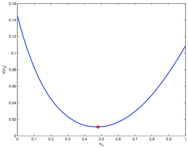
Figure 3. Curve $\eta(\alpha_{4})$ defined by (A.8). The optimal $\alpha_{4}$ which corresponds to the mimimum value of $\eta$ is plotted by a red circle.

The figure 3 presents the evolution of $\eta$ related to $\alpha_{4}\in[0,1]$. The optimal value of $\alpha_{4}$ is plotted by a red circle; it is given by

$$\alpha_{4}=0.4796,$$ (3.1)

that can be compared to the value determined from [Win09]

$$\alpha_{4}^{\text{W}}=0.6260.$$ (3.2)

As assumed previously, this difference is related to the difference in the position of HAT during squat jumping and the position collected on cadavers.

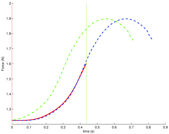
Figure 4. Three methods to determine the ordinate of the center of mass for one subject: the double integration of the experimental force (red continuous line), with synchronized experimental data (blue dashed line), and with non synchronized experimental (dashdot green line). The ordinate of the center of mass determined with synchronized experimental data depend on $\nu$ and $\alpha_{4}$. A green vertical line shows the end of the push-off.

See also figure 4. The ordinates of $G$ determined by synchronized experimental data are close to those determined with the double integration of the experimental force. This is not the case for non synchronized experimental data. This finding validates the synchronization.

3.1.2. Smoothing

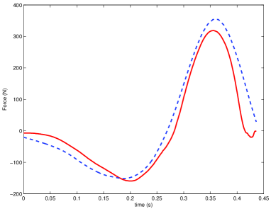
(a) : horizontal ground reaction

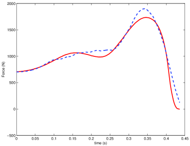
(b) : vertical of ground reaction

Figure 5. Ground reaction determined by two methods: Experimental (red continuous line), and by using a smoothed acceleration of the center of mass (blue dashed line).

Concerning the smoothing, the figure 5 points out that curves of the experimental and calculated reaction force during the push-off phase, are close. From these results, the smoothing developped is considered as valuable.

3.1.3. The three methods and the three degrees

Method A

Table 1. Values of obtained inertia $I_{1}$, $I_{2}$, $I_{3}$ and $I_{4}$ in kgm² for different cases.

case	by values (degree $j=0$) )	by integration (degree $j=1$)	by double integration (degree $j=2$)
$I_{1}$	-21.10836389	9.96412006	13.13320316
$I_{2}$	-9.67961630	10.13963418	12.55758823
$I_{3}$	-1.56382741	0.58549936	1.29624104
$I_{4}$	-3.63374661	8.28949873	9.52771715

Table 2. Values of $\alpha_{i}$,$m_{i}/m$, $\widetilde{r}_{i}$, and $I_{i}$ (in kgm²) according to [Win09].

$i$	$\alpha_{i}$	$m_{i}/m$	$\widetilde{r}_{i}$	$I_{i}$
$1$	0.5000	0.0290	0.4750	0.0116
$2$	0.5670	0.0930	0.3020	0.1104
$3$	0.5670	0.2000	0.3230	0.2890
$4$	0.6260	0.6780	0.4960	4.2067

The calculated IP are presented in Table 1. This method is not valuable while it provides values without any physical meaning. Indeed, we can see that:

1. For $j=0$, obtained values are note positive.

   In this case, we may consider a constrained optimization with inequalities $I_{i}\geq 0$. However, since the unconstrained overdetermined linear problem possesses a unique solution, the constrained optimization problem will give solution where at least one inertia is equal to zero, which is not interesting from a physical viewpoint.

2. For $j=1$ or $j=2$, obtained values differ greatly from values given by [Win09] from table 2.

Then, this method has to be removed.

Method B

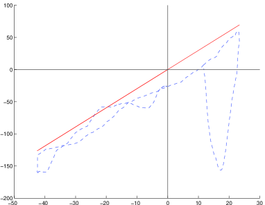
(a) : degree $j=0$

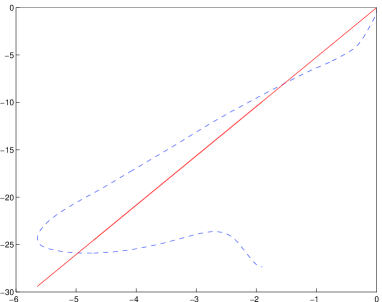
(b) : degree $j=1$

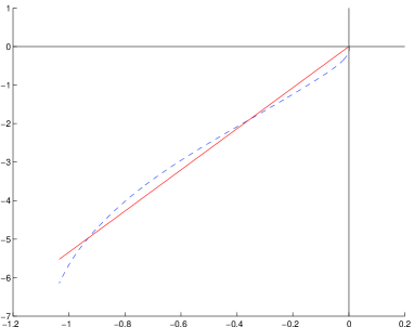
(c) : degree $j=2$

Figure 6. Points $(x_{i},y_{i})$ for different degrees; point $(x_{i},y_{i})$ are plotted with a blue dashed line and points $(x_{i},I_{4}x_{i})$ are plotted with a red continuous line.

From the plotting points $(x_{i},y_{i})$ defined by (2.19) and (2.20) for the three values of $j$ (in figure 6), it can be seen that the best result corresponds to $j=2$. For the Figure 6(c), the slope is equal to $5.32608$. This value is greater to the one obtained from Winter data ($4.2067$). The corresponding value of $\widetilde{r}_{4}$ is equal to

$$\widetilde{r}_{4}=0.5587,$$ (3.3)

it can be compared to the value determined from [Win09]:

$$\widetilde{r}_{4}^{\text{W}}=0.4960.$$ (3.4)

Method C

For this method, inertia are chosen according to Winter (method C).

Comparison bettwen the three methods and the three degrees and conclusion

Table 3. Values of $\varepsilon^{(j)}_{\text{X}}$ for different cases.

degree $j$	method A	method B	method C
0	0.31124363	0.38646452	0.45798897
1	0.06599102	0.25223184	0.25915191
2	0.00308765	0.04714447	0.12324873

Table 4. Values of ${R^{2}}^{(j)}_{\text{X}}$ for different cases.

degree $j$	method A	method B	method C
0	0.54983769	0.24688232	0.10704717
1	0.98053164	0.69054004	0.56793975
2	0.99994990	0.98865321	0.89740132

First of all, for $\varepsilon^{(j)}_{\text{X}}$ (table 3), the lower the value close to 0, the more accurate the method. Concerning ${R^{2}}^{(j)}_{\text{X}}$ (table 4), the more the value is close to 1, the more accurate the method. Therefore, whatever the degree, $\varepsilon^{(j)}_{\text{X}}$ and ${R^{2}}^{(j)}_{\text{X}}$ are less and less accurate from methods A to C. Considering the degree of integration, for the three methods (A to C), the results are more and more precise from degree 0 to degree 2. Finally, for the particular studied subject, the tables 3 and 4 enable to established that the more accurate method was A2, followed by B2 and A1 then by B1. We also see that C2 is more accurate than C0. We note that under the form

$$\text{A2}<\text{B2}<\text{A1}<\text{B1},$$ (3.5a)

$$\text{B2}<\text{B1}<\text{B0},$$ (3.5b)

$$\text{C2}<\text{C0},$$ (3.5c)

where "$<$" means "more accurate than".

The method A can not be applied regarding the values given for inertia $I_{i}$ (see section 3.1.3). Therefore, the best method, physically acceptable is the method B2.

This result will be confirmed by the statistics of section 3.2.2.

3.1.4. Inverse dynamic

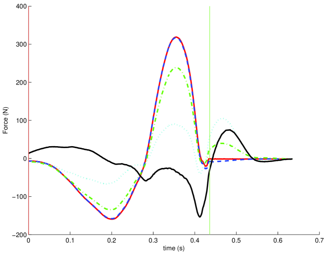
(a) : horizontal joint reaction

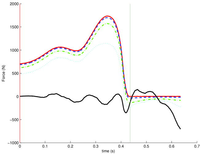
(b) : vertical joint reaction

Figure 7. Differents joint reactions; action from the support on the toe are plotted by a red continuous line, action from the toe on the ankle by a blue dashed line, action from the ankle on knee by dashdot green line, action knee the on the hip by cyan dotted line, and residual action by a black continuous line. The vertical green line corresponds to take off. These values was determined from inertia given by method B2.

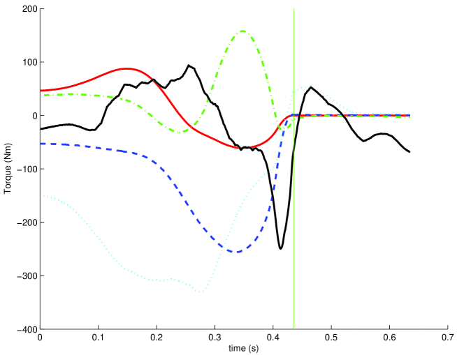
(a) : joint torque

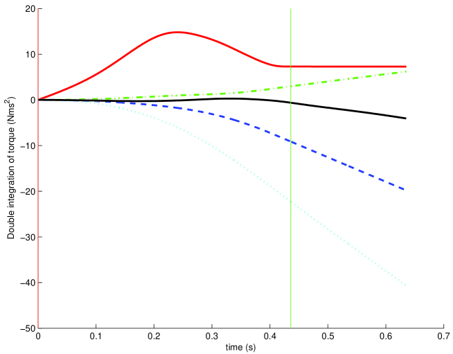
(b) : double integration of joint torque

Figure 8. Differents joint torques; action from the support on the toe are plotted by a red continuous line, action from the toe on the ankle by a blue dashed line, action from the ankle on knee by dashdot green line, action knee the on the hip by cyan dotted line, and residual action by a black continuous line. The vertical green line corresponds to take off. These values was determined from inertia given by method B2.

The results of inverse dynamic methods are plotted on figures 7 and 8 for inertia given by method B2. For all figures, the beginning of the impulsion (corresponding to $t_{0}$) is plotted by a vertical red line and the end of the impulsion (corresponding to $t_{f}$) is plotted by a vertical green line.

On figures 8, the residual torque and their double integrations are plotted. Torque value increased just before the end of impulsion. It can be noticed that the norm $l^{2}$ of the double integral of this torque were optimized but the maximum value of the torque were not optimized. See figure 8(b): the smallest value of the double integrations corresponds to the residual torque.

3.2. Generalization on the population (twelve subjets)

12 subjects performed beetwen 5 and 10 (mean: 7.25) maximal squat jumps, which gave 97 squat jumps. The non positive or greater than 1 values of radius of gyration were removed. Then, the number kept for analysis was 87.

3.2.1. Study of $\alpha_{4}$ and $r_{4}$

We now study $\alpha_{4}$ for trunk.

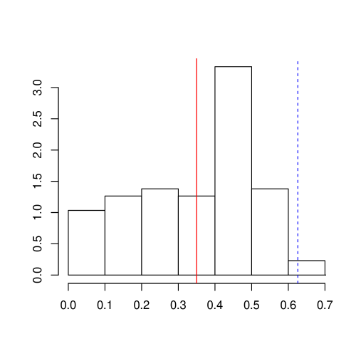
Figure 9. Histogram of $\alpha_{4}$.

See histogram in figure 9. On all figures, we added the mean of data, plotted by a red continuous line, and the value determined by Winter, plotted by a blue dashed line. Here, according to Winter, $\alpha_{4}^{\text{W}}$ is defined by (3.2).

Table 5. Basic statistics for $\alpha_{4}$ and $\widetilde{r}_{4}$

variable	mean	sd	$25\%$ quantile	$75\%$ quantile	$2.5\%(Q_{1})$ quantile	$97.5\%(Q_{3})$ quantile
$\alpha_{4}$	0.3499	0.1858	0.2124	0.4718	0.0011	0.6063
$\widetilde{r}_{4}$	0.5838	0.2206	0.4348	0.7557	0.1753	0.9669

Basic statistics are given in Table 5. We see that $50\%$ of values belong to the interval $[0.2124,0.4718]$ and that $95\%$ of values belong to the interval $[0.0011,0.6063]$.

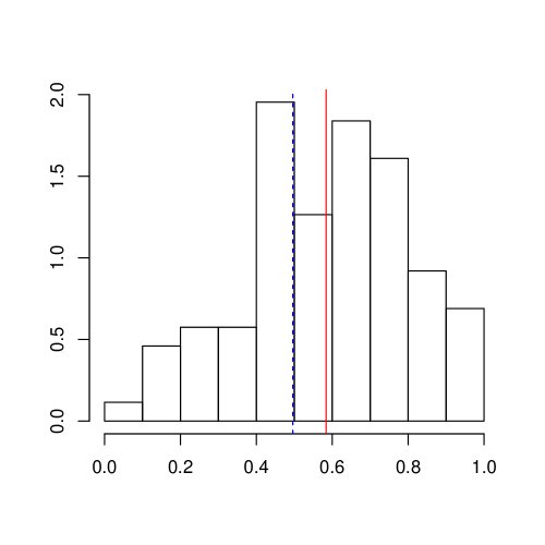
Figure 10. Histogram of $\widetilde{r}_{4}$.

We now study the normalized radius of gyration $\widetilde{r}_{4}$. Here, for Winter, $\widetilde{r}_{4}^{\text{W}}$ is defined by (3.4). See figure 10.

Basic statistics are given in Table 5. We see that $50\%$ of values are included in the interval $[0.4348,0.7557]$ and that $95\%$ of values are included in the interval $[0.1753,0.9669]$.

3.2.2. Comparison beetwen Methods defined by X $\in$ $\{$A,B,C$\}$ and $j\in\{0,1,2\}$

The Shapiro-Wilk test shows that data $\varepsilon_{\text{X}}^{(j)}$ and $1-{R^{2}}^{(j)}_{\text{X}}$ do not present a normal distribution; on the contrary, the logarithm of theses data follow a Gaussian distribution.

Table 6. Groups statistics of $\log_{10}(\varepsilon_{\text{X}}^{(j)})$ for the three studied methods with the three degrees: mean $\pm$ standard deviation.

degree $j$	method A	method B	method C
0	$-0.46\pm 0.16$	$-0.35\pm 0.14$	$-0.28\pm 0.1$
1	$-1.06\pm 0.29$	$-0.59\pm 0.3$	$-0.37\pm 0.25$
2	$-1.83\pm 0.44$	$-1.01\pm 0.38$	$-0.49\pm 0.33$

Table 7. Groups statistics of $\log_{10}\left(1-{R^{2}}^{(j)}_{\text{X}}\right)$ for the three studied methods with the three degrees: mean $\pm$ standard deviation.

degree $j$	method A	method B	method C
0	$-0.27\pm 0.28$	$-0.05\pm 0.23$	$0.11\pm 0.24$
1	$-1.47\pm 0.48$	$-0.52\pm 0.31$	$0.03\pm 0.54$
2	$-2.99\pm 0.73$	$-1.37\pm 0.56$	$-0.2\pm 0.82$

Recall that for $p\in[0,1]$

• ’***’ means $p<0.001$;

• ’**’ means $p<0.01$;

• ’*’ means $p<0.05$;

• ’.’ means $p<.1$.

Statistics on $\log_{10}(\varepsilon_{\text{X}}^{(j)})$ and $\log_{10}\left(1-{R^{2}}^{(j)}_{\text{X}}\right)$ are given in tables 6 and 7. All tables with numerical details are given in Appendix B.1.

First of all, taken into consideration the $\log_{10}$ of $\varepsilon$ and $1-R^{2}$, the lowest the value (close to 0), the more accurate the method or the degree of integration.

Both for $\log_{10}(\varepsilon)$ and $\log_{10}\left(1-R^{2}\right)$, the general linear model one way ANOVA for repeated measures pointed out significant differences between the three methods (A, B and C) and the three degrees (0, 1 and 2) ($p\leq 3.933e-233$ (***)).

Both for $\log_{10}(\varepsilon)$ and $\log_{10}\left(1-R^{2}\right)$ the post- hoc Tuckey tests indicated that for the methods A and B, the values decreased when the degree increased (degree 2 $<$ degree 1 $<$ degree 0, $p<1.856e-08$ (***)). Concerning the method C, the results of $\log_{10}(\varepsilon)$ and $\log_{10}\left(1-R^{2}\right)$ were lower for degree 2 than degree 1 ($p<0.01663$ (*)). No significant difference was observed between the degree 1 and degree 0.

Concerning the comparison of the methods, for the degree 1 and 2, the values of $\log_{10}(\varepsilon)$ the following order was observed: A $<$ B $<$ C (A$<$B$<$C: $p\leq 3.869e-07$ (***). Concerning the values of $\log_{10}\left(1-R^{2}\right)$ were the lowest for method A, then B, then C (A$<$B$<$C, $p\leq 1.205e-13$ (***)). With regard to the degree 0, the method A was significantly lower than method B ($p\leq 0.02942$ (*)). No difference was observed between the other methods.

Finally, when all methods and degrees were compared together, the lowest values of $\log_{10}(\varepsilon)$ and $\log_{10}\left(1-R^{2}\right)$ were observed for method A2. The later was significantly lower than method A1 and method B2. By comparing A1 and B2, we obtain $p\geq 0.2719$. The latter were significantly lower than the method B1. Moreover, if we compare B1 to C2 and C2 to C0, we obtain a maximum value of $p$ value equal to $0.0181$ (*). We denote all theses results under the following form:

$$\text{A2}<\text{B2}=\text{A1}<\text{B1}<\text{C2}<\text{C0},$$ (3.6a)

$$\text{B2}<\text{B1}<\text{B0},$$ (3.6b)

$$\text{A0}<\text{B0},$$ (3.6c)

that confirms the results for one subject (3.5). As shown in the table 1, the results of method A gave unphysical values. Therefore the most accurate method was the method B2.

C0 and C2 are the methods with torque value or double integration of torque corresponding to Winter’s data respectively. A0 and B0 are optimization methods on all IP or only trunk IP with Winter’s data. These two methods would correspond to the choice of methods used by [RHW08, RHW09, DCV07].

Moreover, the geometrical mean of error method A2 is $6.5338$ smaller than the one of B2, what we denote under the form: $\text{A2}/\text{B2}\leq 6.5338$. See appendix B.2 for complete results. We obtain the corroboration of (3.6):

$$\frac{\text{A2}}{\text{B2}}\leq 6.5338,\quad\frac{\text{B2}}{\text{B1}}\leq 2.669,\quad\frac{\text{B1}}{\text{C2}}\leq 1.2634,$$ (3.7a)

$$\frac{\text{C2}}{\text{C0}}\leq 1.5924,\quad\frac{\text{B1}}{\text{B0}}\leq 1.7228,\quad\frac{\text{A0}}{\text{B0}}\leq 1.272.$$ (3.7b)

The error values decrease compared to the previous methods observed in the litterature.

4. Discussion

The purpose of this study was to adjust AP and IP of the human segments during squat jumping in order to minimize error in joint torque. The results indicated that the method A2 minimized the most the residual torque (ie. $\varepsilon$ and $1-R^{2}$) following by the methods B2 and A1 being more accurate than the method B1. Nevertheless, the method A yields unrealistic $I_{j}$, therefore the most accurate method retained was the method B2. Consequently, the optimization focused especially on the HAT inertial and anthropometric parameters. It seems to be possible to optimize AP and IP of one segment when the others are known, but the simultaneous optimization of three AP and IP segments seems to be difficult. According to [RHW09] IP and AP optimized for three segments can not be considered as true, while if two of three segments are known, the IP and AP of the last segment can be calculated.

The IP and AP found with the method B2 are close to the Winter ones but gave better residual joint torque. These differences could be obviously explained by the different position between the subjects performing squat jumps and cadavers. Especially the position of the arms was different, influencing the IP and AP of the HAT segment. [RHW08, RHW09] used optimization techniques to solve inverse dynamic by determining numerical angles which minimize the difference between the ground reaction force measured and the ground reaction force calculated. They found segmental angles which minimize an objective function under equality and inequality constraints, by taking into account the difference ground reaction force measured and the ground reaction force calculated. From these angles, joint torques are determined. Our approach is different: techniques of [RHW08, RHW09] to determine angle and torque were not applied. Only experimental displacements smoothed (see section 2.4) were considered. Then, with a direct inverse method, joint forces and torques were deduced. Finally, an optimization is made on the residual torque and force to determine values of AP and IP. This optimization is very simple and fast, since it is based on the least square linear method (see Eq. (A.11) and (A.12)). It can be noticed that even if the residual torque or force are minimized, the error at each joint may be increased [Kuo98, RHW08, RHW09]. However, in our study and for the method B, we only optimized AP and IP of the trunk, consequently the joint torque and forces at the hip, knee and ankle joints remained unchanged. The major difference with classical way is the following point: it is possible to minimize residual torque, or its integral or its double integral. The best method corresponds to the minimization of the double integral, which do not use the double derivative of angle. Equations (3.6) and (3.7) show that our methods seem to be better than classical one according statistics or error results.

5. Conclusion

The optimization of inertial and anthropometric parameters seems to be necessary when researchers use inverse dynamic methods. Indeed, cadaver data lead to errors in the calculi of the joint torques. These ones could be reduced by optimization methods. The present method of optimization, based on the double integration of residual, has been applied on the HAT segment but could also be applied on more segments. Therefore, further studies focusing on cutting the HAT segment into more segments (the pelvis and the rachis for example) will use this method to calculate the anthropometric and inertial parameters of the new segments composing the HAT.

Appendix A A few theoretical reminders

A.1. Synchronisation of displacements and forces and determination of $\alpha_{4}$

We have

$$\forall t\in[t_{0},t_{f}],\quad\vec{R}=-m\vec{g}+m\frac{d^{2}\overrightarrow{OG}}{dt^{2}}.$$ (A.1)

With this equation, experimental values $\vec{R}$ and the acceleration of $G$, can be compared. Nevertheless, calcul of the acceleration of $G$ from a double derivation of the numerical experimental data leads to inaccuracy; moreover, data are not synchronized. Let introduce the residual force defined by

$$\vec{\widetilde{R}}=\vec{R}+m\vec{g}-m\frac{d^{2}\overrightarrow{OG}}{dt^{2}}.$$ (A.2)

from a theoretical point of view, $\vec{\widetilde{R}}$ should be equal to zero. Experimentally, this residual force is not equal to zero. It depends to $\alpha_{1}$, $\alpha_{2}$, $\alpha_{3}$, which are known (from table 2) and $\alpha_{4}$, unknow. It also depends of the time phase beetwen the forces and the displacements. Then it depends on $\nu$, defined by (2.5). Moreover, to avoid the determination of acceleration of $G$, the double integration of the residual force is applied:

$$\overrightarrow{\mathcal{R}}(t)=\int_{t_{0}}^{t}\int_{t_{0}}^{u}(\vec{R}(s)+m\vec{g})\,dsdu-m\left(\overrightarrow{OG}(t)-\overrightarrow{OG}(t_{0})\right)$$ (A.3)

The measures on $x$-axis are smaller than of the $y$-axis. Then the ordinate of the residual force will be considered

$$\mathcal{R}_{y}(t)=\int_{t_{0}}^{t}\int_{t_{0}}^{u}(R_{y}(s)-mg)\,dsdu-my_{G}(t)+my_{G}(t_{0}),$$ (A.4)

where $y_{G}(t)$ is the ordinate of the center of mass of the body. $\mathcal{R}_{y}(t_{i})$ are defined by

$$\forall i,\quad\mathcal{R}_{y}(t_{i})=\int_{t_{0}}^{t_{i}}\int_{t_{0}}^{u}(R_{y}(s)-mg)\,dsdu-my_{G}(t_{i})+my_{G}(t_{0}).$$ (A.5)

The double integral can be numerically calculated from experimental $R_{y}^{i}$ and from integer $\nu$ defined by (2.5) is the delay between force and displacement and $G(t_{i})$ can be determined according to experimental data $y_{j}^{i}$ (ordinates of anatomical landmarks) and ${{\alpha_{1}}}$, ${{\alpha_{2}}}$, ${{\alpha_{3}}}$, which are known (from table 2) and $\alpha_{4}$, unknow.

If $y={\left(y_{i}\right)}_{1\leq i\leq P}$ is an element of $\mathbb{R}^{P}$, we note by $l^{2}$ norm:

$$\left\|y\right\|=\sqrt{\sum_{i=1}^{P}y_{i}^{2}}.$$ (A.6)

Let $i_{f}$ be a last integer $i$ such that $t_{i}\leq t_{f}$. Then, the number

$$\left\|\mathcal{R}_{y}\right\|=\left\|{\left(\mathcal{R}_{y}(t_{i})\right)}_{0\leq i\leq i_{f}}\right\|,$$ (A.7)

depends on $\alpha_{4}$ and $\nu$. For each value of $\alpha_{4}$, the value of $\nu$, which minimizes $\left\|\mathcal{R}_{y}\right\|$, noted $\eta(\alpha_{4})$, is determined:

$$\forall\alpha_{4}\in[0,1],\quad\eta(\alpha_{4})=\min_{\nu}\left\|\mathcal{R}_{y}\right\|$$ (A.8)

Secondly the value of $\alpha_{4}$ which minimizes $\eta$ is calculated:

$$\eta(\alpha_{4})=\min_{\alpha\in[0,1]}\eta(\alpha).$$ (A.9)

Since $\nu$ and $\alpha_{4}$ are determined, $W_{y}(t)$ is "small" and can be rewritten under the form

$$\int_{t_{0}}^{t}\int_{t_{0}}^{u}\left(\frac{1}{m}R_{y}(s)-g\right)\,dsdu-y_{G}(t)+y_{G}(t_{0})\approx 0$$ (A.10)

which leads to determine then the ordinate of $G$ from three methods:

• with the double integration of the experimental force;

• with synchronized experimental data;

• with non synchronized experimental data.

If experimental forces and displacements are synchronized, the value of $\nu$ is known and $\left\|W_{y}\right\|$ depends only on $\alpha_{4}$. In this case,

$$\mathcal{R}_{y}(t_{i})=A_{i}\alpha_{4}+B_{i},$$

where $A_{i}$ and $B_{i}$ are known. The determination of $\alpha_{4}$ which minimizes $\left\|W_{y}\right\|$ is obtained by solving

$$\forall i,\quad A_{i}\alpha_{4}+B_{i}=0$$

in the least square sens: see appendix A.2.

A.2. Linear least squares system

For integers $P,Q$ such that $P\geq Q$ for all matrix $A\in{\mathcal{M}}_{P,Q}(\mathbb{R})$, for all $B\in\mathbb{R}^{P}$, overdetermined linear system is considered

$$AX=B,$$ (A.11)

in the following sens: find $x\in\mathbb{R}^{Q}$ such that

$$\left\|Ax-B\right\|=\min_{X\in\mathbb{R}^{Q}}\left\|AX-B\right\|.$$ (A.12)

There is a unique solution if the rank of matrix $A$ is equal to $Q$ [LT93]. A system like (A.12) is called a linear least squares system. On a theoretical point of view, the unique solution of (A.11) or (A.12) is given by

$$x={\left({}^{t}AA\right)}^{-1}({}^{t}A)B,$$ (A.13)

where ${}^{t}A$ is the the transpose of the matrix $A$. The matrix ${\left({}^{t}AA\right)}^{-1}({}^{t}A)$ is some times called pseudoinverse of $A$.

A.3. Smoothing of experimental data $x_{j}^{i}$, $y_{j}^{i}$, $x_{G_{j}}^{i}$, $y_{G_{j}}^{i}$, $x_{G}^{i}$ and $y_{G}^{i}$

Since the values of $x_{j}^{i}$, $y_{j}^{i}$, $x_{G_{j}}^{i}$, $y_{G_{j}}^{i}$, $x_{G}^{i}$ and $y_{G}^{i}$, are experimental data, they are not necessarily smooth and can not be derivatived ones or twice.

Then the following smoothing is used: it returns the cubic smoothing spline for the given data $\left({\mathcal{X}}_{i}=i/f,{\mathcal{Y}}_{i}\right)$ ($f$ is the acquisition frequency) and depending on the smoothing parameter $s_{p}\in[0,1]$. This smoothing spline $F$ minimizes

$$s_{p}\sum_{i}\left({\mathcal{Y}}_{i}-F({\mathcal{X}}_{i})\right)^{2}+(1-s_{p})\int(F^{\prime\prime})^{2}.$$

For $s_{p}=0$, the smoothing spline is the least-squares straight line fit to the data, while, at the other extreme, i.e., for $s_{p}=1$, it is the "natural" or variational cubic spline interpolant. The transition region between these two extremes is usually only a rather small range of values for $s_{p}$ and its location strongly depends on the data sites. Smoothing values of data $\left({\mathcal{Y}}_{i}\right)$ are then noted $F_{s_{p}}({\mathcal{X}}_{i})$. The smoothing derivatives of data can be obtained. Moreover, values can be determined for each value of time. Then, it can be assumed that (2.3) and (2.5) hold for the smallest value of the frequency, now noted $f^{\prime}_{e}$. Since time phase $\nu$ is now determined, (2.3) and (2.5) can be replaced by

$$\forall j\in\{1,...,q\},\quad\forall i\in\{0,...,n^{\prime}\},\quad x_{j}^{i}=x_{j}(i/f^{\prime}_{e}),$$ (A.14a)

$$y_{j}^{i}=y_{j}(i/f^{\prime}_{e}),$$ (A.14b)

$$\vec{R}^{i}=\vec{R}(i/f^{\prime}_{e}),$$ (A.14c)

$$C^{i}=C(i/f^{\prime}_{e}).$$ (A.14d)

where $f^{\prime}_{e}=1000$ Hz. is the common acquisition frequency (for force and displacement). The values of displacement, velocity and acceleration of experimental data, $x_{j}^{i}$, $y_{j}^{i}$, $x_{G_{j}}^{i}$, $y_{G_{j}}^{i}$, $x_{G}^{i}$ and $y_{G}^{i}$ are replaced by their smoothing values.

An important choice is the value of each smoothing parameter ${s_{p}}_{j}\in[0,1]$ (for each point $A_{j}$) . The values of ${s_{p}}_{j}\in[0,1]$ which minimize the residual force defined by $\left\|{\widetilde{R}_{x}}\right\|$ and $\left\|{\widetilde{R}_{y}}\right\|$ defined from (A.2) were calculated.

The derivatives of angles defined by (2.2) can be determined.

Appendix B Complete numerical statistical resultats

B.1. ANOVA and post-hoc Tukey tests

Table 8. ANOVA for repeated measures

variable	$F$ value	$p(>F)$
$\log_{10}(\varepsilon)$	308.2546	3.933e-233 (***)
$\log_{10}(1-R^{2})$	390.9661	5.969e-264 (***)

Table 9. Post-hoc Tukey tests on $\log_{10}(\varepsilon)$

	method A		method B		method C
	Estimate	$Pr(<t)$	Estimate	$Pr(<t)$	Estimate	$Pr(<t)$
1 $\leq$ 0	$-0.6086$	$0$ (***)	$-0.2362$	$1.856e-08$ (***)	$-0.0898$	$0.07801$ (.)
2 $\leq$ 1	$-0.7647$	$0$ (***)	$-0.4263$	$0$ (***)	$-0.1123$	$0.01663$ (*)

Table 10. Post-hoc Tukey tests on $\log_{10}\left(1-{R^{2}}\right)$.

	method A		method B		method C
	Estimate	$Pr(<t)$	Estimate	$Pr(<t)$	Estimate	$Pr(<t)$
1 $\leq$ 0	$-1.1917$	$0$ (***)	$-0.4731$	$3.323e-10$ (***)	$-0.0781$	$0.6292$ ( )
2 $\leq$ 1	$-1.5217$	$0$ (***)	$-0.8501$	$0$ (***)	$-0.2238$	$0.006464$ (**)

Table 11. Post-hoc Tukey tests on $\log_{10}(\varepsilon)$.

degree $j$	A $\leq$ B		B $\leq$ C
	Estimate	$Pr(<t)$	Estimate	$Pr(<t)$
0	$-0.1045$	$0.02942$ (*)	$-0.0674$	$0.2618$ ( )
1	$-0.4768$	$0$ (***)	$-0.2138$	$3.869e-07$ (***)
2	$-0.8152$	$0$ (***)	$-0.5279$	$0$ (***)

Table 12. Post-hoc Tukey tests on $\log_{10}\left(1-{R^{2}}\right)$.

degree $j$	A $\leq$ B		B $\leq$ C
	Estimate	$Pr(<t)$	Estimate	$Pr(<t)$
0	$-0.2261$	$0.005771$ (**)	$-0.1545$	$0.09916$ (.)
1	$-0.9448$	$0$ (***)	$-0.5494$	$1.205e-13$ (***)
2	$-1.6164$	$0$ (***)	$-1.1757$	$0$ (***)

Table 13. Post-hoc Tukey tests on $\log_{10}(\varepsilon)$.

test	Estimate	$Pr(<t)$
A1$\leq$ B2	$-0.0505$	$0.2956$ ( )
B1$\leq$ C2	$-0.1015$	$0.01805$ (*)
C2$\leq$ C0	$-0.2021$	$1.001e-06$ (***)

Table 14. Post-hoc Tukey tests on $\log_{10}\left(1-{R^{2}}\right)$.

test	Estimate	$Pr(<t)$
A1$\leq$ B2	$-0.0947$	$0.2719$ ( )
B1$\leq$ C2	$-0.3256$	$1.161e-05$ (***)
C2$\leq$ C0	$-0.302$	$5.039e-05$ (***)

B.2. Decrease of error

We try to compare $\log_{10}(\varepsilon^{(j)}_{\text{X}})$ and $\log_{10}(\varepsilon^{(j^{\prime})}_{\text{X'}})$. If $Q=87$ is the number of measures and if we write, for each measure $i$,

$${\eta}_{i}=\log_{10}\left({\varepsilon^{(j)}_{\text{X}}}_{i}\right)$$

we obtain the geometric mean according to the arithmetric mean

$${\left(\prod_{i}{\varepsilon^{(j)}_{\text{X}}}_{i}\right)}^{1/Q}=10^{\left(\frac{1}{Q}\sum_{i}{\eta}_{i}\right)}=10^{\overline{\log_{10}(\varepsilon^{(j)}_{\text{X}})}}$$

Thus,

$$\frac{{\left(\prod_{i}{\varepsilon^{(j^{\prime})}_{\text{X'}}}_{i}\right)}^{1/Q}}{{\left(\prod_{i}{\varepsilon^{(j)}_{\text{X}}}_{i}\right)}^{1/Q}}=10^{\left(-\overline{\log_{10}(\varepsilon^{(j)}_{\text{X}})}+\overline{\log_{10}(\varepsilon^{(j^{\prime})}_{\text{X'}})}\right)}.$$ (B.1)

It implies that, in geometrical mean, if the difference of the logarithms is equal to $\Delta L$, the error is divided by $10^{\Delta L}$.

By using table 6, we obtain tables 15 and 16

Table 15. Division of error according to method.

degree $j$	A/B	B/C
0	1.272	1.1678
1	2.9979	1.6362
2	6.5338	3.3719

Table 16. Division of error according to degree.

degree $j$	method A	method B	method C
$1/0$	4.0605	1.7228	1.2296
$2/1$	5.8168	2.669	1.2951

References

- [BCSJ08] Maarten F Bobbert, L. J Richard Casius, Igor W T Sijpkens, and Richard T Jaspers. Humans adjust control to initial squat depth in vertical squat jumping. J Appl Physiol, 105(5):1428–1440, Nov 2008.
- [BdGJC06] Maarten F Bobbert, Wendy W de Graaf, Jan N Jonk, and L. J Richard Casius. Explanation of the bilateral deficit in human vertical squat jumping. J Appl Physiol, 100(2):493–499, Feb 2006.
- [CCC+00] C. K. Cheng, H. H. Chen, C. S. Chen, C. L. Chen, and C. Y. Chen. Segment inertial properties of chinese adults determined from magnetic resonance imaging. Clin Biomech (Bristol, Avon), 15(8):559–566, Oct 2000.
- [Che08] Kuangyou B Cheng. The relationship between joint strength and standing vertical jump performance. J Appl Biomech, 24(3):224–233, Aug 2008.
- [CHLT11] S.-C. Chen, H.-J. Hsieh, T.-W. Lu, and C.-H. Tseng. A method for estimating subject-specific body segment inertial parameters in human movement analysis. Gait and Posture, 33:695–700, 2011.
- [CMY69] C.E. Clauser, I.T McConville, and I.W. Young. Weight, volume and center of mass of segments of the human body. Wright-Paterson A.F.B., Ohio, 1969. (AMRL-TR-69-70).
- [CSY78] R.F. Chandler, R. Snow, and J.W Young. Computation of mass distribution characteristics of children. B. Soc. of Photo-Optical Instrumentation Engineers, Washington, 1978.
- [DC07] Zachary J Domire and John H Challis. The influence of squat depth on maximal vertical jump performance. J Sports Sci, 25(2):193–200, Jan 2007.
- [DC10] Zachary J Domire and John H Challis. An induced energy analysis to determine the mechanism for performance enhancement as a result of arm swing during jumping. Sports Biomech, 9(1):38–46, Mar 2010.
- [DCV07] R. Dumas, L. Chèze, and J-P. Verriest. Adjustments to mcconville et al. and young et al. body segment inertial parameters. J Biomech, 40(3):543–553, 2007.
- [Dem55] W.T Dempster. Space requirements of the seated operator. Techn. Report WADC-TR-55-159., 1955. Ohio (WADC-TR-55-159): Wright-Paterson AFB.
- [Dur98] J.L. Durkin. The prediction of body segment paramters using geometric modelling and dual photon absorptiometry. McMaster University: Hamilton, Ontario, 1998.
- [FHO+99] E. G. Fowler, D. M. Hester, W. L. Oppenheim, Y. Setoguchi, and R. F. Zernicke. Contrasts in gait mechanics of individuals with proximal femoral focal deficiency: Syme amputation versus van nes rotational osteotomy. J Pediatr Orthop, 19(6):720–731, 1999.
- [Fuj63] K. Fujikawa. The center of gravity in the parts of human body. Okajimas Folia Anat Jpn, 39:117–125, Jul 1963.
- [GRF08] Evan J Goldberg, Philip S Requejo, and Eileen G Fowler. The effect of direct measurement versus cadaver estimates of anthropometry in the calculation of joint moments during above-knee prosthetic gait in pediatrics. J Biomech, 41(3):695–700, 2008.
- [Hat02] H Hatze. Anthropomorphic contour approximation for use in inertial limb parameter computation. In 12th international conference on mechanics in medecine and biology, Lemnos, 2002.
- [Hin85] R. N. Hinrichs. Regression equations to predict segmental moments of inertia from anthropometric measurements: an extension of the data of chandler et al. (1975). J Biomech, 18(8):621–624, 1985.
- [Hin90] R. N. Hinrichs. Adjustments to the segment center of mass proportions of clauser et al. (1969). J Biomech, 23(9):949–951, 1990.
- [HLM06] Marianne Haguenauer, Pierre Legreneur, and Karine M Monteil. Influence of figure skating skates on vertical jumping performance. J Biomech, 39(4):699–707, 2006.
- [Hof92] A. L. Hof. An explicit expression for the moment in multibody systems. J Biomech, 25(10):1209–1211, Oct 1992.
- [HS83] H. K. Huang and F. R. Suarez. Evaluation of cross-sectional geometry and mass density distributions of humans and laboratory animals using computerized tomography. J Biomech, 16(10):821–832, 1983.
- [HSAF08] Mikiko Hara, Akira Shibayama, Hiroshi Arakawa, and Senshi Fukashiro. Effect of arm swing direction on forward and backward jump performance. J Biomech, 41(13):2806–2815, Sep 2008.
- [HST+08] Mikiko Hara, Akira Shibayama, Daisuke Takeshita, Dean C. Hay, and Senshi Fukashiro. A comparison of the mechanical effect of arm swing and countermovement on the lower extremities in vertical jumping. Hum Mov Sci, 27(4):636–648, Aug 2008.
- [KTC+95] I. Kingma, H.M. Toussaint, D.A.C.M. Commissaris, M.J.M. Hoozemans, and M.J. Ober. Optimizing the determination of the body center of mass. Journal of Biomechanics, 28:1137–1142, 1995.
- [Kuo98] A. D Kuo. A Least-Squares Estimation Approach to Improving the Precision of Inverse Dynamics Computations. ASME J. Biomech. Eng, 120(1):148–159, 1998.
- [LBD05] Guillaume Laffaye, Benoît G Bardy, and Alain Durey. Leg stiffness and expertise in men jumping. Med Sci Sports Exerc, 37(4):536–543, Apr 2005.
- [LBD07] G. Laffaye, B. G. Bardy, and A. Durey. Principal component structure and sport-specific differences in the running one-leg vertical jump. Int J Sports Med, 28(5):420–425, May 2007.
- [LRC+00] A. Lees, J. Rojas, M. Ceperos, V. Soto, and M. Gutierrez. How the free limbs are used by elite high jumpers in generating vertical velocity. Ergonomics, 43(10):1622–1636, Oct 2000.
- [LT93] P. Lascaux and R. Théodor. Analyse numérique matricielle appliquée à l’art de l’ingénieur. Tome 1. Masson, Paris, second edition, 1993. Métodes directes. [Direct methods].
- [LVC04] Adrian Lees, Jos Vanrenterghem, and Dirk De Clercq. The maximal and submaximal vertical jump: implications for strength and conditioning. J Strength Cond Res, 18(4):787–791, Nov 2004.
- [LVD04] Adrian Lees, Jos Vanrenterghem, and Dirk De Clercq. Understanding how an arm swing enhances performance in the vertical jump. J Biomech, 37(12):1929–1940, Dec 2004.
- [MCK+80] J. T. McConville, T. D. Churchill, I. Kaleps, C. E. Clauser, and J. Cuzzi. Anthropometric relationships of body and body segment moments of inertia. Technical Report AFAMRL-TR-80-119, Aerospace Medical Research Laboratory, Dayton, Ohio: Wright-Patterson Air Force Base, 1980.
- [MMML89] P. E. Martin, M. Mungiole, M. W. Marzke, and J. M. Longhill. The use of magnetic resonance imaging for measuring segment inertial properties. J Biomech, 22(4):367–376, 1989.
- [PC99] D. J. Pearsall and P. A. Costigan. The effect of segment parameter error on gait analysis results. Gait Posture, 9(3):173–183, Jul 1999.
- [PGD96] A. Plamondon, M. Gagnon, and P. Desjardins. Validation of two 3-D segment models to calculate the net reaction forces and moments at the L5/S1 joint in lifting. Clinical Biomechanics, 11, 1996.
- [PR94] D. J. Pearsall and J. G. Reid. The study of human body segment parameters in biomechanics. an historical review and current status report. Sports Med, 18(2):126–140, Aug 1994.
- [PRL96] D. J. Pearsall, J. G. Reid, and L. A. Livingston. Segmental inertial parameters of the human trunk as determined from computed tomography. Ann Biomed Eng, 24(2):198–210, 1996.
- [R D11] R Development Core Team. R: A Language and Environment for Statistical Computing. R Foundation for Statistical Computing, Vienna, Austria, 2011. ISBN 3-900051-07-0.
- [RHW08] Raziel Riemer and Elizabeth T Hsiao-Wecksler. Improving joint torque calculations: optimization-based inverse dynamics to reduce the effect of motion errors. J Biomech, 41(7):1503–1509, 2008.
- [RHW09] Raziel Riemer and Elizabeth T Hsiao-Wecksler. Improving net joint torque calculations through a two-step optimization method for estimating body segment parameters. J Biomech Eng, 131(1):011007, Jan 2009.
- [RJ90] J. G. Reid and R. K. Jensen. Human body segment inertia parameters: a survey and status report. Exerc Sport Sci Rev, 18:225–241, 1990.
- [VAH82] C. L. Vaughan, J. G. Andrews, , and J. G. Hay. Selection of body segment parameters by optimization methods. ASME J. Biomech. Eng., pages 38–44, 1982.
- [VLL+04] Jos Vanrenterghem, Adrian Lees, Matthieu Lenoir, Peter Aerts, and Dirk De Clercq. Performing the vertical jump: movement adaptations for submaximal jumping. Hum Mov Sci, 22(6):713–727, Apr 2004.
- [Win09] David Winter. Biomechanics and Motor Control of Human Movement. John Wiley and Sons, New York, fourth edition, 2009.
- [WYK07] Cassie Wilson, Maurice R Yeadon, and Mark A King. Considerations that affect optimised simulation in a running jump for height. J Biomech, 40(14):3155–3161, 2007.
- [YM89] M. R. Yeadon and M. Morlock. The appropriate use of regression equations for the estimation of segmental inertia parameters. J Biomech, 22(6-7):683–689, 1989.
- [ZS83] V.M. Zatsiorsky and V.N. Seluyanov. The mass and iniertia characteritics of the main segments of the human body. Champaign: Humain Kinetics, 1983. in Biomechanics VIII-B, p. 1152-1159.