Three-Dimensional MHD Simulations of Emerging Active Region Flux in a Turbulent Rotating Solar Convective Envelope: the Numerical Model and Initial Results

Abstract

We describe a 3D finite-difference spherical anelastic MHD (FSAM) code for modeling the subsonic dynamic processes in the solar convective envelope. A comparison of this code with the widely used global spectral anlastic MHD code, ASH (Anelastic Spherical Harmonics), shows that FSAM produces convective flows with statistical properties and mean flows similar to the ASH results. Using FSAM, we first simulate the rotating solar convection in a partial spherical shell domain and obtain a statistically steady, giant-cell convective flow with a solar-like differential rotation. We then insert buoyant toroidal flux tubes near the bottom of the convecting envelope and simulate the rise of the flux tubes in the presence of the giant cell convection. We find that for buoyant flux tubes with an initial field strength of 100 kG, the magnetic buoyancy largely determines the rise of the tubes although strong down flows produce significant undulation and distortion to the shape of the emerging $\Omega$-shaped loops. The convective flows significantly reduce the rise time it takes for the apex of the flux tube to reach the top. For the weakly twisted and untwisted cases we simulated, the apex portion is found to rise nearly radially to the top in about a month, and produce an emerging region (at a depth of about 30 Mm below the photosphere) with an overall tilt angle consistent with the active region tilts, although the emergence pattern is more complex compared to the case without convection. Near the top boundary at a depth of about 30 Mm, the emerging flux shows a retrograde zonal flow of about 345 m/s relative to the mean flow at that latitude.

1 Introduction

If we believe that active regions on the solar surface originate from a strong toroidal magnetic field generated at the base of the convection zone by the solar dynamo mechanism, then we need to understand how active-region-scale flux tubes rise through the turbulent solar convection zone to the surface. Recently significant insight has been gained in this area from a series of work (Weber et al., 2011, 2012) conducted using a thin flux tube model driven via the drag force term by a time dependent giant-cell convective flow with a solar like differential rotation, computed separately from a 3D global convection simulation with the Anelastic Spherical Harmonic (ASH) code (Miesch et al., 2006). Because of the low computational cost for the 1-D thin flux tube model, a large number of simulations of rising flux tubes with a range of initial field strengths, fluxes, initial latitudes, and sampling different time spans of the convective flow field were carried out. Meaningful statistics on the properties of the emerging tubes in regard to the latitude of emergence, tilt angles, apparent zonal motion, and clustering in longitudes of emergence (i.e. active longitudes) is obtained. It is found that the dynamic evolution of the flux tube changes from convection dominated to magnetic buoyancy dominated as the initial field strength increases from 15 kG to 100 kG. At 100 kG, the development of $\Omega$-shaped rising loops is mainly controlled by the growth of the magnetic buoyancy instability, with the strongest convective downdrafts capable of producing moderate undulations on the emerging loops. It is found that although helical convection promotes mean tilts towards the observed Joy’s law trend, results still favor stronger fields ($>40$ kG) for the initial toroidal tubes to avoid too large a tilt angle scatter produced by convection to be consistent with the observations (Weber et al., 2012).

Although the thin flux tube model essentially preserves the frozen-in condition for the evolution of the flux tube and allows for a large number of simulations to achieve meaningful statistics, it is highly idealized. It ignores the 3D nature of the magnetic field evolution and assumes the tube is a cohesive object. In parallel to the thin flux tube calculations, several self-consistent 3D global MHD simulations of rising flux tubes in a rotating spherical shell of solar convection and the associated mean flows have been carried out (Jouve & Brun, 2009; Jouve et al., 2013) using the ASH code. These simulations study rather large flux tubes (significantly greater than the flux contained in typical active regions) due to the limited numerical resolutions in the global scale simulations. It is found that the rise velocity and the characteristics of the emerging loops are strongly affected by the convective motions when loops of less than $10^{5}$ G are considered. In addition, the question of how strong buoyant flux tubes can self-consistently form from dynamo generated mean field and rise to the surface is also being addressed in a set of full global convective dynamo simulations of a fast rotating stellar envelope with 3 times the solar rotation rate (Nelson et al., 2011, 2013a, 2013b), also using the ASH code.

In this paper, we describe a new 3D Finite-difference Spherical Anelastic MHD (FSAM) code for modeling the subsonic dynamics of the turbulent solar convective envelope. The code uses a modified Lax-Friedrichs scheme (as described in the Appendix) for computing the upwinded fluxes in the advection terms, which allows for stable numerical integration of the anelastic MHD equation with no explicit diffusion. Of course numerical diffusion is present, but is minimized in smooth regions which helps to preserve the frozen-in condition of the magnetic field evolution in the simulations of rising flux tubes. We carry out a comparison between the FSAM code and the ASH code with a simulation of rotating convective flow in a spherical shell. We find that even with the absence of the polar region (necessary due to the polar singularity associated with the latitude-longitude grid discretization), the FSAM code can produce convective flows with similar statistical properties and mean flow properties as the fully global ASH spectral code. We then use the FSAM code to conduct a simulation of rotating solar convection in a spherical shell wedge domain driven at the lower boundary by the diffusive heat flux corresponding to the solar luminosity. We obtain a statistically steady solution of giant-cell convection with a solar-like differential rotation. Into the giant-cell convective flow, we then insert buoyant toroidal flux tubes with an initial field strength of $10^{5}$ G near the bottom of the envelope, to study how the tubes rise under the presence of convection. We find that the buoyant loops rise based on the initial magnetic buoyancy distribution and also are significantly reshaped by the strong convective downdrafts. They can rise to the surface nearly radially, and produce emerging regions with radial flux distribution of the two polarities that are consistent with the observed mean tilt angles of solar active regions. At a depth of about 30 Mm below the photosphere, the emerging flux shows a retrograde zonal motion in the midst of the prograde flow of the banana cells, with a speed of $\sim-350$ m/s relative to the mean plasma zonal flow at the emerging latitude.

2 The Numerical Model

We solve the following anelastic MHD equation in a spherical shell domain:

$$\nabla\cdot(\rho_{0}{\bf v})=0,$$ (1)

$$\rho_{0}\left[\frac{\partial{\bf v}}{\partial t}+({\bf v}\cdot\nabla){\bf v}\right]=2\rho_{0}{\bf v}\times{\bf\Omega}-\nabla p_{1}+\rho_{1}{\bf g}+\frac{1}{4\pi}(\nabla\times{\bf B})\times{\bf B}+\nabla\cdot{\cal D}$$ (2)

$$\rho_{0}T_{0}\left[\frac{\partial s_{1}}{\partial t}+({\bf v}\cdot\nabla)(s_{0}+s_{1})\right]=\nabla\cdot(K\rho_{0}T_{0}\nabla s_{1})-({\cal D}\cdot\nabla)\cdot{\bf v}+\frac{1}{4\pi}\eta(\nabla\times{\bf B})^{2}-\nabla\cdot{\bf F}_{\rm rad}$$ (3)

$$\nabla\cdot{\bf B}=0$$ (4)

$$\frac{\partial{\bf B}}{\partial t}=\nabla\times({\bf v}\times{\bf B})-\nabla\times(\eta\nabla\times{\bf B}),$$ (5)

$$\frac{\rho_{1}}{\rho_{0}}=\frac{p_{1}}{p_{0}}-\frac{T_{1}}{T_{0}},$$ (6)

$$\frac{s_{1}}{c_{p}}=\frac{T_{1}}{T_{0}}-\frac{\gamma-1}{\gamma}\frac{p_{1}}{p_{0}},$$ (7)

where $s_{0}(r)$, $p_{0}(r)$, $\rho_{0}(r)$, $T_{0}(r)$, and ${\bf g}=-g_{0}(r){\hat{\bf r}}$ denote the profiles of entropy, pressure, density, temperature, and the gravitational acceleration of a time-independent, reference state of hydrostatic equilibrium and nearly adiabatic stratification, $c_{p}$ is the specific heat capacity at constant pressure, $\gamma$ is the ratio of specific heats, and ${\bf v}$, ${\bf B}$, $s_{1}$, $p_{1}$, $\rho_{1}$, and $T_{1}$ are the dependent variables of velocity, magnetic field, entropy, pressure, density, and temperature to be solved that describe the changes from the reference state. In equation (2), ${\bf\Omega}$ denotes the solid body rotation rate of the Sun and is the rotation rate of the frame of reference, where $\Omega=2.7\times 10^{-6}{\rm rad}\;{\rm s}^{-1}$, and ${\cal D}$ is the viscous stress tensor:

$${\cal D}_{ij}=\rho_{0}\nu\left[S_{ij}-\frac{2}{3}(\nabla\cdot{\bf v})\delta_{ij}\right],$$ (8)

where $\nu$ is the kinematic viscosity, $\delta_{ij}$ is the unit tensor, and $S_{ij}$ is given by the following in spherical polar coordinates:

$$S_{rr}=2\frac{\partial v_{r}}{\partial r}$$ (9)

$$S_{\theta\theta}=\frac{2}{r}\frac{\partial v_{\theta}}{\partial\theta}+\frac{2v_{r}}{r}$$ (10)

$$S_{\phi\phi}=\frac{2}{r\sin\theta}\frac{\partial v_{\phi}}{\partial\phi}+\frac{2v_{r}}{r}+\frac{2v_{\theta}}{r\sin\theta}\cos\theta$$ (11)

$$S_{r\theta}=S_{\theta r}=\frac{1}{r}\frac{\partial v_{r}}{\partial\theta}+r\frac{\partial}{\partial r}\left(\frac{v_{\theta}}{r}\right)$$ (12)

$$S_{\theta\phi}=S_{\phi\theta}=\frac{1}{r\sin\theta}\frac{\partial v_{2}}{\partial\phi}+\frac{\sin\theta}{r}\frac{\partial}{\partial\theta}\left(\frac{v_{\phi}}{\sin\theta}\right)$$ (13)

$$S_{\phi r}=S_{r\phi}=\frac{1}{r\sin\theta}\frac{\partial v_{r}}{\partial\phi}+r\frac{\partial}{\partial r}\left(\frac{v_{\phi}}{r}\right).$$ (14)

Futhremore, $K$ in equation (3) denotes the thermal diffusivity, and $\eta$ in equations (5) and (3) denotes the magnetic diffusivity. The last term in equation (3) is a heating source term due to the radiative diffusive heat flux ${\bf F_{\rm rad}}$ in the solar interior, where

$${\bf F_{\rm rad}}=\frac{16\sigma_{s}{T_{0}}^{3}}{3\kappa\rho_{0}}\nabla T_{0},$$ (15)

and $\sigma_{s}$ is the Stephan-Boltzman constatn, $\kappa$ is the Rosseland mean opacity.

Using equations (6) and (7) to express $\rho_{1}$ in terms of $p_{1}$ and $s_{1}$ in equation (2), and after some manipulations using the ideal gas law and hydrostatic balance for the reference state, we obtain

$$\rho_{0}\left[\frac{\partial{\bf v}}{\partial t}+({\bf v}\cdot\nabla){\bf v}\right] = 2\rho_{0}{\bf v}\times{\bf\Omega}-\rho_{0}\nabla\left(\frac{p_{1}}{\rho_{0}}\right)+\rho_{0}g_{0}\frac{s_{1}}{c_{p}}{\hat{\bf r}}$$ (16)

$$+\frac{1}{4\pi}(\nabla\times{\bf B})\times{\bf B}+\nabla\cdot{\cal D}.$$

Note, in deriving the above equation, we have ignored terms of higher order in $\delta$, where

$$\delta\equiv\frac{{\rm d}\ln T_{0}}{{\rm d}\ln p_{0}}-\frac{\gamma-1}{\gamma}$$ (17)

is the non-dimensional super-adiabaticity of the reference stratification, and its magnitude is $\ll 1$ in the anelatic approximation. The super-adiabaticity $\delta$ is related to the entropy gradient of the reference state as follows:

$$\frac{{\rm d}s_{0}}{{\rm d}r}=-c_{p}\frac{\delta}{H_{p0}},$$ (18)

where

$$H_{p0}=-\left(\frac{{\rm d}\ln p_{0}}{{\rm d}r}\right)^{-1}$$ (19)

denotes the pressure scale height.

To ensure the divergence free condition of equation (1) is satisfied, $p_{1}$ in equation (16) needs to satisfy the following linear elliptic equation, which we solve at every time step before using it in the above momentum equation to advance ${\bf v}$:

$$\nabla\cdot\left[\rho_{0}\nabla\left(\frac{p_{1}}{\rho_{0}}\right)\right]=\nabla\cdot{\cal F}$$ (20)

where

$${\cal F}=-\rho_{0}{\bf v}\cdot\nabla{\bf v}+2\rho_{0}{\bf v}\times{\bf\Omega}+\rho_{0}g_{0}\frac{s_{1}}{c_{p}}{\hat{\bf r}}+\frac{1}{4\pi}(\nabla\times{\bf B})\times{\bf B}+\nabla\cdot{\cal D}.$$ (21)

Also applying the divergence free condition of equation (1), we can rewrite the entropy equation as follows:

$$\rho_{0}T_{0}\frac{\partial s_{1}}{\partial t} = -\nabla\cdot[\rho_{0}{\bf v}T_{0}(s_{1}+s_{0})]-\rho_{0}v_{r}(s_{1}+s_{0})\frac{g_{0}}{c_{p}}$$ (22)

$$+\rho_{0}\nu\left[{S_{r\theta}}^{2}+{S_{\theta\phi}}^{2}+{S_{\phi r}}^{2}+\frac{1}{6}((S_{rr}-S_{\theta\theta})^{2}+\left(S_{\theta\theta}-S_{\phi\phi})^{2}+(S_{\phi\phi}-S_{rr})^{2}\right)\right]$$

$$+\eta(\nabla\times{\bf B})^{2}+\nabla\cdot(K\rho_{0}T_{0}\nabla s_{1})+\nabla\cdot\left(\frac{16\sigma_{s}{T_{0}}^{3}}{3\kappa\rho_{0}}\nabla T_{0}\right).$$

In deriving the above equation, we have used

$$\frac{{\rm d}T_{0}}{{\rm d}r}=-\frac{g_{0}}{c_{p}}$$ (23)

where we have ignored the terms of order $O(\delta)$ produced by the small superadiabaticity in the reference profile of $T_{0}$ and only preserved the zeroth order term (corresponding to the adiabatic stratification). The viscous heating term, which is positive definite, has also been written out explicitly in terms of the tensor components $S_{ij}$.

Thus, in summary, we numerically solve equations (16), (20), (22), and (5), to advance the dependent variables ${\bf v}$, $p_{1}$, $s_{1}$, and ${\bf B}$. A more detailed description of the numerical schemes used to solve these equations is given in the appendix. We further note that by summing ${\bf v}\cdot$ equation (16), ${\bf B}\cdot$ equation (5), and equation (22), we can also obtain the following equation for total energy conservation:

$${\partial\over\partial t}\left(\rho_{0}\frac{v^{2}}{2}+\rho_{0}T_{0}s_{1}+\frac{B^{2}}{8\pi}\right)$$ (24)

$$= -\nabla\cdot\left[\left(\rho_{0}\frac{v^{2}}{2}+p_{1}+\rho_{0}T_{0}(s_{1}+s_{0})\right){\bf v}-\frac{1}{4\pi}({\bf v}\times{\bf B})\times{\bf B}\right]-\rho_{0}v_{r}s_{0}\frac{g_{0}}{c_{p}}$$

$$+\nabla\cdot({\bf v}\cdot{\cal D})+\nabla\cdot\left[-\eta(\nabla\times{\bf B})\times{\bf B}\right]$$

$$+\nabla\cdot\left(K\rho_{0}T_{0}\nabla s_{1}\right)+\nabla\cdot\left(\frac{16\sigma_{s}{T_{0}}^{3}}{3\kappa\rho_{0}}\nabla T_{0}\right).$$

Since numerically we are solving the entropy equation (22) instead of the above total energy equation explicitly in conservative form, the total energy equation can serve as an independent check on the effects of numerical dissipation.

3 A comparison of FSAM and ASH

Were FSAM to include the polar caps, we could assess the accuracy of its results by direct comparison against the hydrodynamic anelastic benchmark solution of Jones et al. (2011). The benchmark solution is most appropriate for solution domains encompassing the full sphere as it manifests as a sectoral mode of convection, localized around the equator, and propagating prograde with time. Unfortunately, we find that the absence of a polar region in FSAM alters the meridional circulations achieved in the benchmark solution, ultimately preventing FSAM from obtaining the pure spherical harmonic mode of convection achievable when the full sphere is simulated.

One major use of FSAM is for studies of magnetic flux emergence through a turbulent solar convection zone, and while benchmarks are of some interest, we are most concerned with its ability to yield convective motions with properties similar to those thought to exist in the Sun. To this end, we have chosen to run a somewhat more turbulent simulation and compare the properties of the solution against those obtained using the Anelastic Spherical Harmonic (ASH) code. ASH solves the three-dimensional (3-D) anelastic MHD equations in deep spherical shells using a pseudospectral approach. It employs a spherical harmonic expansion in the horizontal direction, and Chebyshev polynomials or a finite-difference approach in the radial direction. ASH has been used extensively to model the solar convection zone (e.g. Brun et al., 2004; Miesch et al., 2008), and has shown good agreement with other anelastic codes when applied to the benchmark problems of Jones et al. (2011). By comparing the results of FSAM against ASH in a somewhat more turbulent regime than the weakly non-linear benchmark test in Jones et al. (2011), we anticipate that the properties of the convective flows in the bulk of the solution is less affected by the role played by the polar region.

3.1 Experimental Setup

We have constructed a comparison experiment by modeling convection in a spherical shell spanning the full depth of the solar convection zone, albeit with a much reduced density stratification relative to the Sun. We assume that the gravitational acceleration $g_{0}(r)$ varies as $GM_{int}/r^{2}$ within the shell, where $M_{int}$ is the mass interior to the base of the convection zone and $G$ is the gravitational constant, and use the following adiabatically stratified, polytropic atmosphere as the reference state:

$$\rho_{0}=\rho_{i}\left(\frac{\zeta}{\zeta_{i}}\right)^{n},~{}~{}~{}~{}T_{0}=T_{i}\frac{\zeta}{\zeta_{i}},~{}~{}~{}~{}p_{0}=p_{i}\left(\frac{\zeta}{\zeta_{i}}\right)^{n+1},$$ (25)

where the subscript “i” denotes the value of a quantity at the inner boundary, and n is the polytropic index. The radial variation of the reference state is captured by the variable $\zeta$, defined as

$$\zeta=c_{0}+\frac{c_{1}d}{r},$$ (26)

where $d=r_{o}-r_{i}$ is the depth of the convection zone. The constants $c_{0}$ and $c_{1}$ are given by

$$c_{0}=\frac{2\zeta_{o}-\beta-1}{1-\beta},~{}~{}~{}~{}c_{1}=\frac{(1+\beta)(1-\zeta_{o})}{(1-\beta)^{2}},$$ (27)

with

$$\zeta_{o}=\frac{\beta+1}{\beta\mathrm{exp}(N_{\rho}/n)+1},~{}~{}~{}~{}\zeta_{i}=\frac{1+\beta-\zeta_{o}}{\beta}.$$ (28)

Here $\zeta_{i}$ and $\zeta_{o}$ are the values of $\zeta$ on the inner and outer boundaries, $\beta=r_{i}/r_{o}$, and $N_{\rho}$ is the number of density scale heights across the shell. Further details of this model setup may be found in Jones et al. (2011).

We choose to employ this description for the reference state, with a density variation of one scale height across the shell. Entropy ($s_{1}$) is fixed at both the upper and lower boundary with a constant entropy difference $\Delta S$ across the domain, allowing us to specify a Rayleigh number. Our model further differs from the Sun in that radiative heating by photon diffusion (the last term on the right hand side of eq. [22]), particularly important near the base of the convection zone, is neglected. The thermal energy throughput of the system is instead entirely determined by thermal conduction (the 2nd to last term on the right hand side of eq. [22]) at the boundaries. The degree of thermal conduction may vary in time (due to the changes in $\partial s_{1}/\partial r$ at the boundaries), but reaches a statistically steady state that is itself determined by the entropy gradients established by the convection. Our thermal diffusivity $K$ and viscosity $\nu$ are taken to be constant functions of depth with a Prandtl number $P_{r}$ of unity. Values for the simulation parameters are provided in Table 1.

For the ASH simulation, we used 200 points in radius, and chose a maximum spherical harmonic degree of 170, yielding an effective resolution of 200$\times$256$\times$512 ($r$,$\theta$,$\phi$). To assess the effects of resolution and polar region removal, we chose to run three distinct FSAM simulations. These three simulations were identical in every respect except for spatial resolution and domain size. The primary simulation (case A), employed a resolution that is approximately half that of the ASH simulation, with a resolution of 96$\times$128$\times$256, and extended to $\pm$60^∘ in latitude. Case B extended over the same latitude range, but employed a resolution of 192$\times$256$\times$512 (twice that of case A). Case C extended from $\pm$75^∘ in latitude, and employed a resolution of 96$\times$160$\times$256 (similar to case A). With the exception of case B, each simulation was evolved for 4000 days (about seven thermal and viscous diffusion times) to ensure that a thermally and dynamically well-equilibrated state was obtained. The somewhat more expensive Case B was evolved for 1200 days (about two thermal diffusion times).

3.2 Convective Morphology

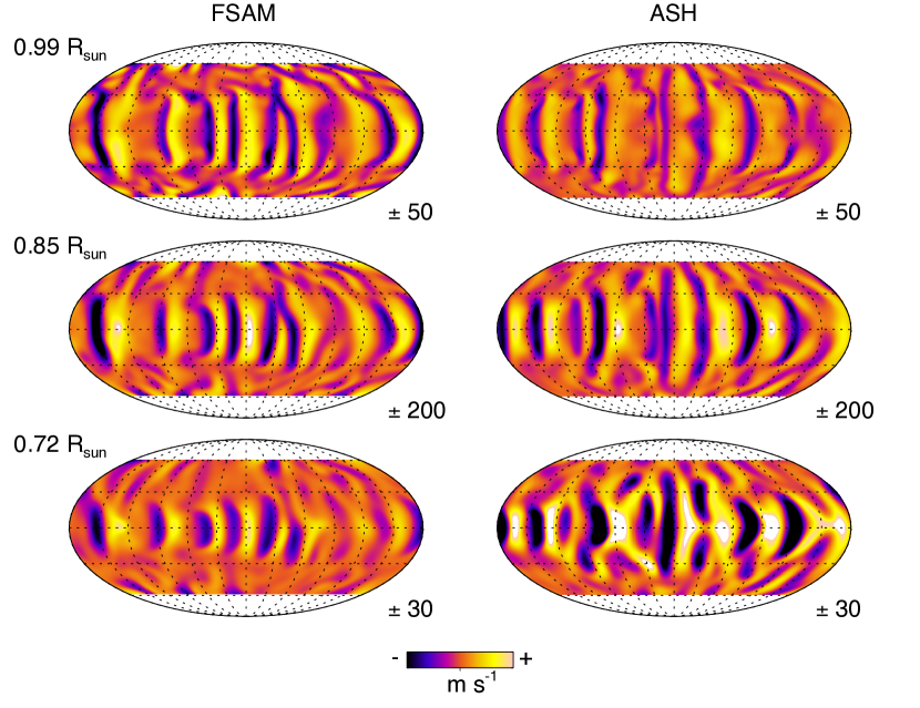
Figure 1: Radial velocity $v_{r}$ at three depths from FSAM case A and the ASH simulation, shown in Mollweide projection. Horizontal lines indicate lines of constant latitude, and curved arcs lines of constant longitude. Regions of yellow denote upflows, and regions of blue indicate downflows. Flows in FSAM are stronger near the surface and weaker near the bottom than their counterparts in ASH. Banana cell patterns in ASH tend to reach to higher latitudes than those in FSAM.

A survey of the radial flows realized in ASH and case A is illustrated in Figure 1. Here snapshots of radial velocity $v_{r}$, taken at three depths from one instant in time near the end of each simulation, are shown. We have omitted the polar regions of ASH in this plot for ease of comparison. Near-surface flow structures are similar in ASH and FSAM results, with flows in both simulations achieving amplitudes of roughly 50 m s^-1 at the top of the domain. Banana cell-like patterns are prominent at the equator in each simulation, but extend to somewhat higher latitudes in the ASH results, possibly due to the inclusion of the polar regions. At mid-convection zone, flows are comparable in amplitude, but the disparity in latitudinal extent of the banana cells has grown, and near the base of the simulation, the solutions are markedly different. Radial flows in FSAM at this depth are both weaker than those realized in ASH and are largely confined to a much narrower equatorial region.

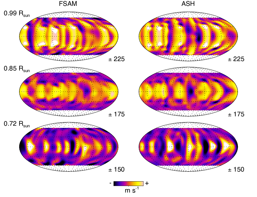
Figure 2: Zonal velocity $v_{\phi}$ plotted at three depths in each simulation at the same time instant as Fig. 1. Azimuthal flows in FSAM case A are similar to those of ASH throughout most of the convection zone, becoming somewhat stronger near the surface.

The zonal velocity $v_{\phi}$ for each simulation is shown in Figure 2. Both simulations develop a prograde differential rotation at the equator. Flow amplitudes compare at depth in a similar manner to the radial flows, with the prograde region of differential rotation occupying a smaller latitudinal extent near the base of the convection zone in the FSAM results than in the ASH results. There are two effects that contribute to the differences in these two solutions, the most obvious of which is the absence of a polar region in FSAM. Moreover, the numerical diffusion scheme employed in FSAM, which operates in addition to the explicit diffusivities, can lead to differing results where the simulation is under-resolved.

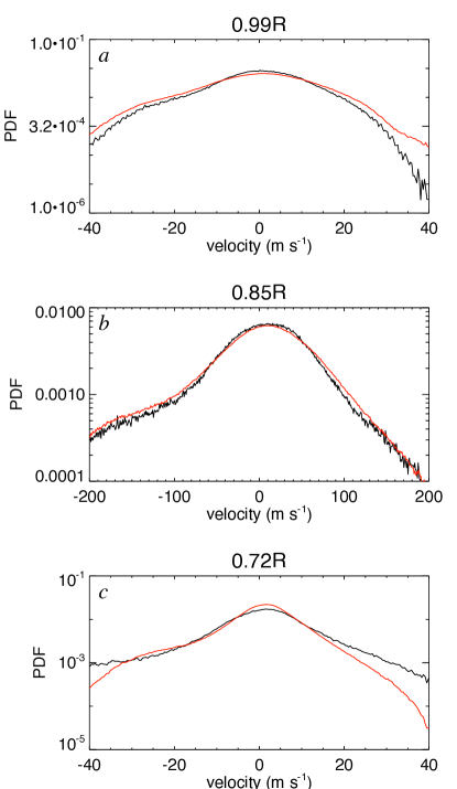
Figure 3: Probability distribution functions (PDF) taken near (a) the top, (b) middle, and (c) bottom of each simulation, averaged in time over 10 rotation periods. PDFs for FSAM case A are shown in red. PDFs for ASH are plotted in black and have been computed over the FSAM range of latitudes. Both simulations show good agreement in the mid-convection zone. The cores of the distributions agree well in the boundary layers, though the wings are stronger for FSAM in the upper boundary layer and weaker relative to ASH in the lower boundary layer.

These snapshots of the flow are from but one instant in each simulation. A sense of how the two solutions compare in a statistical sense may be better gained by looking at probability distribution functions (PDFs) of radial velocity. Figure 3 depicts PDFs of $v_{r}$, averaged over 500 days of evolution at the end of each simulation, and shown at the same three depths as Figure 1. Case A (red) exhibits substantially higher power in the wings of its PDF near the surface than does ASH. At mid-convection zone, the two distributions are in much better agreement, although the FSAM simulation still exhibits somewhat stronger wings. Near the base of the convection zone, where the flows are noticiably different in Figure 1, the ASH flows exhibit significantly stronger wings.

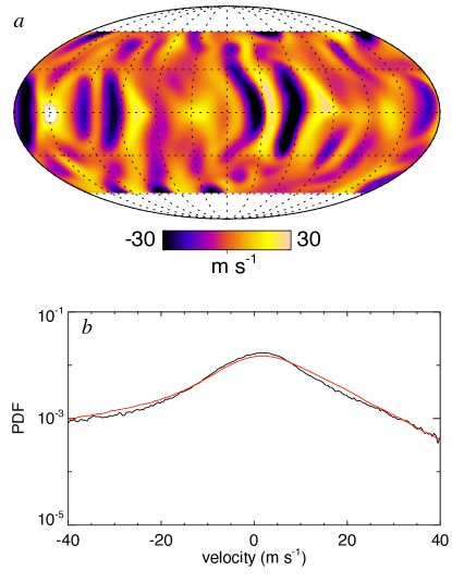
Figure 4: The effect of doubling the spatial resolution. (a) Radial velocity $v_{r}$ from FSAM case B near the bottom of the convection zone (0.72R). Flows are noticiably stronger than case A and extend to higher latitudes when the spatial resolution is doubled. (b) PDFs of radial velocity (at 0.72R) for FSAM case B (red), and the ASH simulation (black). The high velocity wings of the distribution have been enhanced substantially with respect to case A, reaching good agreement with those of the ASH simulation.

We find that these differences in the lower convection zone are substantially diminished when the spatial resolution of the simulation is doubled. We suspect that flow structures associated with convective downdrafts impacting the impenetrable lower boundary are under-resolved in case A, especially in the horizontal dimensions where the resolution is about 4 times worse than the vertical resolution. Figure 4$a$ depicts $v_{r}$ near the base of the convection zone for FSAM case B, which has twice the spatial resolution of case A. Flow amplitudes and structure sizes are comparable to the ASH case for case B. The PDF for $v_{r}$ at the base of the convection zone for case B (Figure 4$b$, red line) is also close to that of the ASH simulation (black line). Interestingly, the high power wings present in case A in the upper portion of the domain are still present in the PDF of case B (not shown). These appear to be related instead to an overdriving of the FSAM systems relative to ASH that arises from removal of the polar regions, a subtle effect that we discuss shortly.

3.3 Mean Flows and Thermodynamics of the System

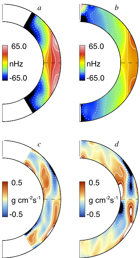
Figure 5: Mean flows averaged in longitude and over 10 rotation periods. (a) Differential rotation as realized with FSAM case A and (b) ASH. The differential rotation established in FSAM is somewhat stronger than that realized in ASH. (c) Latitudinal mass flux achieved in FSAM and (b) ASH. Blue (red) tones indicated poleward flow in the northern (southern) hemisphere, while red (blue) tones indicate equatorward flow. Individual hemispheres tend to be dominated by a large circulation cell for each simulation.

Convective flows realized in FSAM case A and ASH possess mean components that are similar in nature to one another. Figure 5 depicts the mean differential rotation and meridional circulations from each simulation. Case A exhibits a prograde differential rotation at the equator, similar to that of ASH. Meridional circulations in each case are predominantly poleward in the upper convection zone and equatorward at the base of the convection zone. Closer inspection reveals that both simulations tend to develop small counter cells of circulation in the near-surface equatorial regions. The differential rotation of case A, however, is noticiably stronger than that realized in ASH. This enhanced differential rotation realized in FSAM is consistent with its convection being driven more strongly than that of ASH, as suggested by the velocity PDFs. As convection becomes more vigorous, the resulting banana cells become more efficient at establishing a prograde equator in systems such as these where the rotational influence is strong.

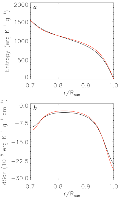
Figure 6: Mean entropy profiles (a) and entropy gradients (b) established in each case. ASH results are plotted in black, and FSAM case A in red. Convection in the FSAM simulations tends to build a somewhat more adiabatic interior and steeper entropy gradients near the boundaries than ASH.

The disparity in convective driving becomes evident when looking at the thermodynamic properties of these systems. Figure 6$(a)$ depicts the time-averaged, spherically symmetric entropy perturbations attained by each simulation. The profiles are similar, but convection in case A (red) tends to build steeper gradients in the boundary layers than that of ASH (black). This is more readily apparent when looking at the entropy gradient (Figure 6$(b)$) for the two simulations. The flows established by FSAM tend to establish an entropy gradient that is 10$\%$ stronger near both the top and bottom boundaries than that established in ASH, while maintaining a more nearly adiabatic interior throughout the bulk of the convection zone. An enhanced entropy gradient near the boundaries translates directly into an increase in the thermal energy throughput of the system.

3.4 The Role of The Polar Regions

How might the difference in convective driving between the two systems arise? For constant entropy boundary conditions, convection is allowed to set the latidudinal profile of the heat flux at the boundaries. In the presence of rotation, convective transport is preferentially more efficient at the high latitudes (e.g. Elliott et al., 2000) where Coriolis constraints on radial motions are weakest. With the polar regions absent, convection in FSAM has less freedom to establish such latitudinal asymetries, and therefore leads to stronger driving of the convective motions at the lower latitudes, and subsequently to stronger banana cell-like structures.

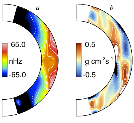
Figure 7: Mean flows averaged in longitude and over 10 rotation periods for FSAM case C. (a) Differential rotation realized when a higher latitude range is included shows reduced amplitude relative to case A, yielding better agreement with the ASH simulation. (b) Latitudinal component of mass flux for case C. Blue (red) tones indicated poleward flow in the northern (southern) hemisphere, while red (blue) tones indicate equatorward flow. Meridional flows in case C also show good agreement with ASH.

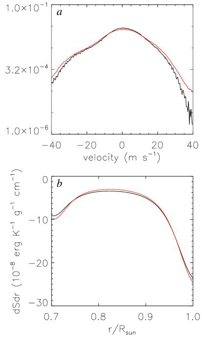
Figure 8: (a) PDFs of $v_{r}$ for FSAM case C (red) and the ASH case (black) near the top of the simulation (0.99R). The inclusion of higher latitudes yields a PDF in case C that is in better agreement with the ASH results than case A. (b) Mean entropy gradients established in case C (red) and the ASH case (black). The superadiabaticity of the boundary layers present in case A is diminished as more latitudes are included in the simulation.

Extension of the latitudinal boundaries to $\pm$75^∘, as we have done with case C, allows us to examine this effect. We find that in this regime, FSAM results begin to converge toward those of ASH. Figure 7 depicts the mean flows for case C. Meridional circulations are very similar to those of the ASH simulation, and the strength of the differential rotation, while still stronger than in ASH, is diminished relative to case A. The wings of the velocity PDF for case C (Figure 8$a$) have come down substantially from their counterparts in case A, most noticiably so in the downflows. Moreover, the steep entropy gradients that developed near the boundaries of case A have diminished in case C relative to case A (Figure 8$b$.)

These tests suggest that FSAM, when properly resolved, can produce convective flows in accord with those produced by the more widely used ASH code. We find reasonable convergence between the full- and partial-sphere simulations as the latitudinal extent of the simulation is increased. On the other hand, these tests suggests that we may be well-cautioned to carefully consider the luminosity we adopt for our simulations. Otherwise we may inadvertently overdrive the convection. As the level of turbulence is increased, however, convection tends to become more homogeneous in latitude (e.g. Gastine et al., 2012; Featherstone et al., 2013) and we expect the role of the absent poles to be diminished in the more turbulent regimes.

4 Buoyant Rise of Active Region Flux Tubes in a Solar Like Convective Envelope

4.1 A simulation of rotating solar convection

We now proceed to carry out a hydrodynamic simulation to obtain a statistically steady solution of a solar like, rotating convective flow field in a spherical shell domain with $r\in[r_{i},r_{o}]$, spanning from $r_{i}=0.722R_{\odot}$ at the base of the convection zone (CZ) to $r_{o}=0.971R_{\odot}$ at about 20 Mm below the photosphere, $\theta\in[\pi/2-\Delta\theta,\pi/2+\Delta\theta]$ with $\Delta\theta=\pi/3$, and $\phi\in[0,2\pi]$. The domain is resolved by a grid with 96 grid points in $r$, 512 grid points in $\theta$, and 768 grid points in $\phi$. The grid is uniform in $r$, $\theta$, and $\phi$ respectively. J. Christensen-Dalsgaard’s solar model (Christensen-Dalsgaard et al., 1996), commonly known as Model S, is used for the reference profiles of $T_{0}$, $\rho_{0}$, $p_{0}$, $g_{0}$ in the simulation domain. We assumed that $s_{0}=0$ for the reference state, i.e. is isentropic. We also omit the heating term due to radiative diffusion $\nabla\cdot{\bf F}_{\rm rad}$ in the CZ in equation (22), but instead, drive convection by imposing at the lower boundary a fixed entropy gradient $\partial s_{1}/\partial r$ such that the solar luminosity $L_{s}$ is forced through the lower boundary as a diffusive heat flux:

$$\left(K\rho_{0}T_{0}\frac{\partial s_{1}}{\partial r}\right)_{r_{i}}=\frac{L_{s}}{4\pi{r_{i}}^{2}}$$ (29)

where $K=2\times 10^{13}\,{\rm cm}^{2}\,{\rm s}^{-1}$ in our simulation domain. We also impose a latitudinal variation of entropy at the lower boundary:

$$\left(\frac{\partial s_{1}}{\partial\theta}\right)_{r_{i}}=\frac{ds_{i}(\theta)}{d\theta}$$ (30)

where

$$s_{i}(\theta)=-\Delta s_{i}\cos\left(\frac{\theta-\pi/2}{\Delta\theta}\pi\right),$$ (31)

to represent the tachocline induced entropy variation that can break the Taylor-Proudman constraint in the convective envelope. In the above we set $\Delta s_{i}=215.7\>{\rm erg}\>{\rm g}^{-1}\>{\rm K}^{-1}$. For the initial condition, we let the initial $s_{1}$ be:

$$s_{1}|_{t=0}=<\!\!s_{1}\!\!>_{t=0}+s_{i}(\theta)-<\!\!s_{i}(\theta)\!\!>$$ (32)

where $<\,>$ denotes the horizontal average at a constant $r$, and $<\!\!s_{1}\!\!>_{t=0}$ is given by:

$$K\rho_{0}T_{0}\frac{d<\!\!s_{1}\!\!>_{t=0}}{dr}=\frac{L_{s}}{4\pi r^{2}},$$ (33)

such that initially the constant solar luminosity is being carried through the solar convection zone by thermal diffusion. This results in an unstable initial stratification, and with a small initial velocity perturbation, convection ensues in the domain. For the upper boundary $s_{1}$ is held fixed to its initial value, while at the lower boundary the fixed gradient of $\partial s_{1}/\partial r$ given by equation (29) maintains a conductive heat flux corresponding to the solar luminosity through the lower boundary. The latitudinal gradient of $s_{1}$ given by equation (30) is also imposed at the lower boundary, but the horizontally averaged value of $s_{1}$ is allowed to change with time. At the two $\theta$ boundaries, $s_{1}$ is assumed symmetric. The velocity field is non-penetrating and stress free at the top, bottom and the two $\theta$-boundaries. The top and bottom boundary condition for $p_{1}$ is

$$\rho_{0}\frac{\partial}{\partial r}\left(\frac{p_{1}}{\rho_{0}}\right)={\cal F}_{r}$$ (34)

at $r=r_{i}$ and $r_{o}$, and ${\cal F}_{r}$ is the $r$-component of ${\cal F}$ given in equation (21). At the two $\theta$-boundaries

$$\frac{\rho_{0}}{r}\frac{\partial}{\partial\theta}\left(\frac{p_{1}}{\rho_{0}}\right)={\cal F}_{\theta},$$ (35)

and ${\cal F}_{\theta}$ is the $\theta$-component of ${\cal F}$ given in equation (21). All quantities are naturally periodic at the $\phi$ boundaries. The kinematic viscosity $\nu=10^{12}\,{\rm cm}^{2}\,{\rm s}^{-1}$ in the simulation domain. This gives a Prandlt number of $Pr=0.05$ for our simulation. The reference frame rotation rate $\Omega$ in equation (16) is set to $2.7\times 10^{-6}\,{\rm rad}\,s^{-1}$, and with respect to this frame, the initial velocity is essentially zero with a very small initial perturbation.

With the above setup of the simulation, we let the convection in the domain evolve to a statistical steady state, which is reached after about $6000$ days. The final steady state entropy gradient reached by the rotating solar convective envelope is shown in Figure 9. The horizontally averaged entropy gradient reaches a value of about $-7.5\times 10^{-6}\,{\rm erg}\,{\rm K}^{-1}\,{\rm cm}^{-1}$ near the top boundary at about $0.97R_{s}$, which is of a similar order of magnitude as the entropy gradient ($\sim 10^{-5}\,{\rm erg}\,{\rm K}^{-1}\,{\rm cm}^{-1}$) at this depth obtained by Model S (Christensen-Dalsgaard et al., 1996). Figure 10 shows the steady state, horizontally integrated total heat flux due to convection:

$$H_{\rm conv}=\frac{4\pi r^{2}}{A(r)}\int_{0}^{2\pi}\int_{\pi/2-\Delta\theta}^{\pi/2+\Delta\theta}\rho_{0}T_{0}v_{r}s_{1}\,r^{2}\,d\theta d\phi$$ (36)

and conduction

$$H_{\rm cond}=\frac{4\pi r^{2}}{A(r)}\int_{0}^{2\pi}\int_{\pi/2-\Delta\theta}^{\pi/2+\Delta\theta}K\rho_{0}T_{0}\frac{\partial s_{1}}{\partial r}\,r^{2}\,d\theta d\phi$$ (37)

where $A(r)$ is the total area of the spherical surface at radius r

$$A(r)=\int_{0}^{2\pi}\int_{\pi/2-\Delta\theta}^{\pi/2+\Delta\theta}\,r^{2}\,d\theta d\phi.$$ (38)

In the above, the total heat fluxes $H_{\rm conv}$ and $H_{\rm cond}$ have been scaled up to the values for the area of a full sphere so that they can be compared directly with the solar luminosity $L_{s}$. Here the conductive heat flux represents the heat transport due to turbulent diffusion by unresolved convection. It can be seen from Figure 10 that with the large value of $K$ used, the solar luminosity is mostly carried through by thermal conduction and the heat flux transported by the resolved convective flow is only a small fraction ($\sim 20$%) of the solar luminosity. In this way the convective flow speed for the resolved giant cell convection is not too high, (even with a relatively low viscosity $\nu=10^{12}\,{\rm cm}^{2}\,{\rm s}^{-1}$ used), so that the convective flow is sufficiently rotationally constrained to allow the maintainance of a solar-like differential rotation with faster equator than the polar regions (e.g Featherstone & Miesch, 2012). The relatively low viscocity is chosen so that the subsequent simulations of the buoyant rise of active region flux tubes are not in a too viscous regime.

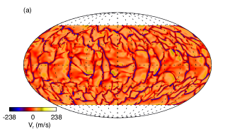
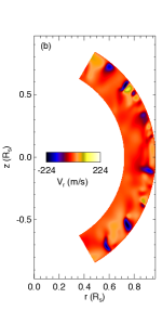
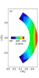
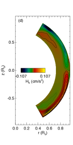
Figure 11: (a) A snapshot of the radial velocity of the rotating solar convection at a depth of about 30 Mm below the photosphere, shown on the full sphere in Mollweide projection. (b) A meridional slice of the radial velocity of the convective flow at the same time. (c and d) Time and azimuthally averaged angular rate of rotation $\Omega$ and kinetic helicity $H_{k}$ in the convective envelope after it has reached the statistical steady state.

Figure 11a shows a snapshot of the radial velocity field of the rotating solar convection at a depth of about 30 Mm below the photosphere displayed on the full sphere in Mollweide projection. It shows giant-cell convection patterns with broad upflows in the network of narrow downflow lanes, and with columnar, rotationally aligned cells (banana cells) at low latitudes. The time and azimuthally averaged mean zonal flow (Figure 11c) shows a solar-like differential rotation profile with faster rotation at the equator and slower rotation towards the poles, and more conical shaped contours of constant angular speed of rotation at mid-latitude range. Figure 11d shows the time and azimuthally averaged kinetic helicity $H_{k}={\bf v}\cdot(\nabla\times{\bf v})$ of the flow. It shows predominantly negative (positive) kinetic helicity in the upper 1/3 to 1/2 of the CZ in the northern (southern) hemisphere and weakly positive (negative) kinetic helicity in the deeper depths of the CZ. The depth of the upper layer with predominantly negative (positive) $H_{k}$ in the northern (southern) hemisphere is relatively shallow because, as can be seen in Figure 11b, the concerntrated downflow plumes do not penetrate very deep. They generally reach less than half of the total depth of the CZ before starting to diverge and leading to a reversal of the kinetic helicity.

4.2 Simulations of Rising Flux Tubes

4.2.1 Simulation Setup

Into the statistically-steady, rotating convective flow with a self-consistently maintained solar like differential rotation, we insert buoyant toroidal flux tubes near the bottom of the CZ to study how they rise through the CZ. The initial flux tube we insert into the convecting domain is given by the following:

$${\bf B}=\nabla\times\left({A(r,\theta)\over r\sin\theta}\hat{\bf\phi}\right)+B_{\phi}(r,\theta)\hat{\bf\phi},$$ (39)

where

$$A(r,\theta)={1\over 2}qa^{3}B_{t}\exp\left(-{\varpi^{2}(r,\theta)\over a^{2}}\right),$$ (40)

$$B_{\phi}(r,\theta)={aB_{t}\over r\sin\theta}\exp\left(-{\varpi^{2}(r,\theta)\over a^{2}}\right).$$ (41)

$$\varpi=(r^{2}+r_{0}^{2}-2rr_{0}\cos(\theta-\theta_{0}))^{1/2}.$$ (42)

In the above, $q$ is the rate of twist (angle of field line rotation about the axis per unit length of the tube), $a$ denotes the e-folding radius of the tube, $r_{0}$ and $\theta_{0}$ are respectively the initial $r$ and $\theta$ values of the tube axis. For all of the simulations of this paper, $a=6.7\times 10^{8}{\rm cm}$ which is about 0.12 times the pressure scale height at the base of the solar convection zone, $r_{0}=5.2\times 10^{10}{\rm cm}$ is at approximately $0.757R_{\odot}$, $\theta_{0}$ corresponds to $15^{\circ}$ latitude, and the initial field strength at the axis of the toroidal flux tube is $B_{t}a/(r_{0}\sin\theta_{0})=10^{5}{\rm G}$. Thus the total flux in the initial toroidal flux tube is $1.4\times 10^{23}$ Mx, which is about a factor of 10 greater than the typical flux in a solar active region. Due to the limited numerical resolution of our global scale simulations of the convective envelope, we can only consider tubes with a rather large cross-section in order for it to be resolved by the numerical grid. In our current simulations the initial tube diameter is resolved by about 7 grid points.

We consider initially buoyant toroidal flux tubes, and specify the initial buoyancy along the tube in the following two ways. In one way, an initial sinusoidal variation (with an azimuthal wavelength of $\pi/2$ in $\phi$) of entropy:

$$\delta s_{1}=c_{p}\left(1-{1\over\gamma}\right){B_{\phi}^{2}\over 8\pi p_{0}}\left[{1\over 2}\left(1-{1\over{\gamma-1}}\right)-{1\over 2}\left(1+{1\over{\gamma-1}}\right)\cos(4\phi)\right]$$ (43)

is being added to the original $s_{1}$ of the convective flow field at the location of the toroidal tube. Thus along each $\pi/2$ azimuthal segment of the toroidal tube, the tube is varying from being (approximately) in thermal equilibrium with the surrounding and thus buoyant, to being approximately in neutral buoyancy. The peak buoyancy in the initial tube is approximately $B_{\phi}^{2}/8\pi H_{p0}$, corresponding to the magnetic buoyancy associated with a flux tube in thermal equilibrium with its surrounding. Another initial buoyancy state we used is to specify a uniform buoyancy along the tube, by adding

$$\delta s_{1}=c_{p}\left(1-{1\over\gamma}\right){B_{\phi}^{2}\over 8\pi p_{0}}$$ (44)

to the original $s_{1}$ of the convective flow field at the location of the toroidal tube. In this way it is uniformly buoyant along the tube with the magnetic buoyancy $B_{\phi}^{2}/8\pi H_{p0}$. We run two simulations of rising flux tubes in the convective flows with the sinusoidal initial buoyancy (eq. [43]), one with a weak initial (left-handed) twist rate of $q=-0.15a^{-1}$, and the other with no initial twist $q=0$. We name these runs “SbWt” (Sinusoidal-buoyancy-Weak-Twist) and “SbZt” (Sinusoidal-buoyancy-Zero-twist) respectively. As a reference for these two simulations, we run two corresponding simulations of the same initial buoyant tubes in a quiescent rotating envelope with no convective flows, but with the same reference stratification of $p_{0}$, $\rho_{0}$, and $T_{0}$. These two runs are named “SbWt-ref” and “SbZt-ref”. Furthermore, we run a simulation (named “UbZt”) of the uniformly buoyant initial tube (using eq. [44]) with no initial twist rising in the convective flow. A summary of these runs is given in Table 2. In this paper we only conduct these few sample runs to examine qualitatively how a solar-like rotating convective flow may influence the rise of relatively strong ($100$ kG) buoyant flux tubes. The peak Alfvén speed $v_{a}$ in the initial flux tube is $764$ m/s. Compared to the convective flow speeds shown in Figure 12, the flux tube is significantly super-equipartition with respect to the mean kinetic energy of the convective flows as reflected by the RMS velocity. However, as discussed in Fan et al. (2003), the hydrodynamic forces from the convective flows would be able to counteract the magnetic buoyancy of the flux tube if the speed of the convective flows is $\,\lower 3.0pt\hbox{$\sim$}\hbox to0.0pt{\hss\raise 2.0pt\hbox{$>$}}\,(a/H_{p})^{1/2}v_{a}$ which is $\sim 265$ m/s considering the initial radius $a$ of the buoyant toroidal flux tubes in the present simulations. Figure 12 shows that the peak downflow speed exceeds that value for most of the convection zone, indicating that the downflow plumes can significantly impede the buoyant rise of the flux tube even for the $100$ kG strong flux tubes considered here.

For the simulations of the rising flux tubes, we preserve the kinematic viscosity $\nu=10^{12}\,{\rm cm}^{2}\,{\rm s}^{-1}$ used for the simulation of the rotating convective flow solution in the entire simulation domain. The thermal diffusivity used in the original convection simulation is much greater ($2\times 10^{13}\,{\rm cm}^{2}\,{\rm s}^{-1}$). This large value is used in order to achieve a solar like differential rotation profile (fast equator, slow poles) in the rotating convection solution. For the rising flux tube simulations, we apply a magnetic field strength dependent quenching of $K$:

$$K=\frac{K_{0}}{1+(B/B_{\rm cr})^{2}}$$ (45)

where $K_{0}=2\times 10^{13}\,{\rm cm}^{2}\,{\rm s}^{-1}$ is the original value of the diffusivity used in the convection simulation and $B_{\rm cr}=100$ G represents a low threshhold field strength above which quenching of thermal diffusion begins to take place. Convection is expected to be suppressed by the strong magnetic field in the flux tube, thus $K$, which represents unresolved eddy diffusion, should be suppressed in the rising flux tubes. For the magnetic field, we also do not include any explicit resistivity $\eta$ in the simulation, so only numerical diffusion is present. This way we minimize magnetic diffusion to preserve the frozen-in condition of the buoyant flux tube as much as possible, given the numerical resolution.

4.2.2 Results

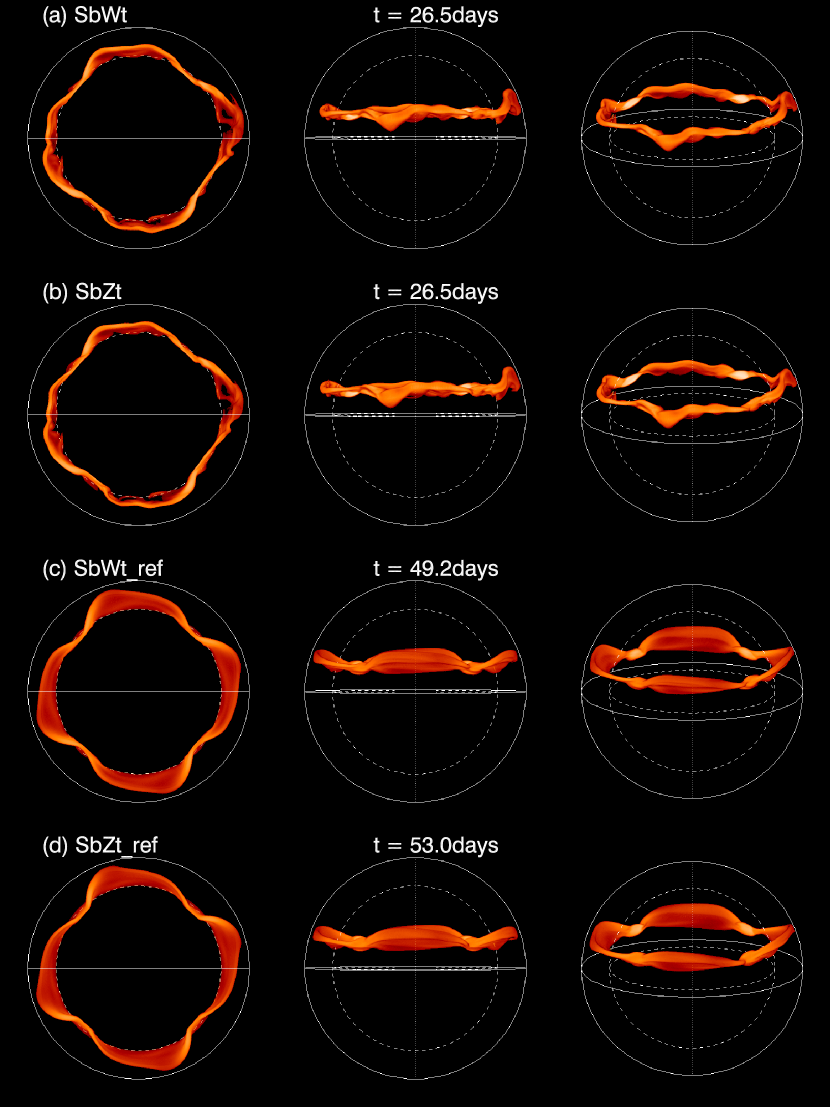
Figure 13: 3D volume rendering of the absolute magnetic field strength of the rising flux tubes developed from simulations SbWt (a), SbZt (b), SbWt-ref (c), and SbZt-ref(d) when an apex of the tube has reached the top boundary. Animations of the evolution of the tube for each simulations are available in the online version of the paper.

Figures 13a and 13b show the rising flux tubes that have developed from the SbWt and SbZt simulations respectively, when an apex of the tube has reached the top boundary. For comparison, the resulting rising tubes from the corresponding reference simulations SbWt-ref and SbZt-ref (without convection) are shown in Figures 13c and 13d. MPEG movies of the evolution of the tube for each of the simulations are available in the online version of the paper. In the absence of convection, four identical rising loops develop due to the initial buoyancy prescription and rise to the top of the domain. Convective flows are found to produce additional undulations on the rising loops, pushing down certain portions while promoting the rise of other portions. With convection, the rise time for an apex of the tube to reach the top is significantly reduced (for example, changed from about 49 days for SbWt-ref to 26.5 days for SbWt).

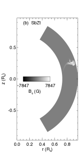
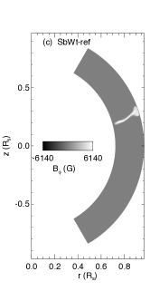
Figure 14: $B_{\phi}$ in the meridional plane at the longitude of the apex location for cases SbWt (a), SbZt (b) , SbWt-ref (c), and SbZt-ref (d) at the same corresponding times shown in Figure 13

There is little difference in the morphology of the rising tubes (at least as shown in the volume rendering of the absolute magnetic field strength) between the weakly twisted and the untwisted cases, both with and without convection. One of the reasons for this is that the twist is rather weak, about a half of the necessary twist rate required for a cohesive rise of the flux of the original flux tube as a whole, similar to the weakly twisted case studied in Fan (2008) (see the LNT case shown in Figure 8 of that paper). In other words, the magnetic energy density associated with the initial twist component of the field (i.e. the $B_{\theta}$ and $B_{r}$ components in the initial toroidal flux tube) is smaller than the kinetic energy density associated with the relative velocity between the tube and the surrounding plasma. As a result the initial twist does not have a great effect on maintaining the cohesion of the rising tube compared to the untwisted case. There is continued flux loss during the rise, forming a track of flux behind the rising apex, as can be seen in the meridional cross-section of $B_{\phi}$ at the apex longitude for all the cases as shown in Figure 14. We also note that the current simulations of the rising flux tubes are in a fairly laminar regime. The Reynolds number for the rising flux tube estimated based on the tube diameter $D\sim 10^{9}$ cm, typical rise speed attained $V_{\rm rise}\sim 100$ m/s, and the viscosity $\nu=10^{12}\,{\rm cm}^{2}/{\rm s}$ (kept the same as that used for obtaining the rotating convection solution), is $R_{e}=V_{\rm rise}D/\nu\sim 10$. Such a low Reynolds number reduces the production of small scale features and fragmentation of the flux tube and thus generally improves the cohesion for the rising flux, especially for the untwisted case. This is also a reason for the reduced difference in the magnetic field morphology between the untwisted and weakly twisted cases.

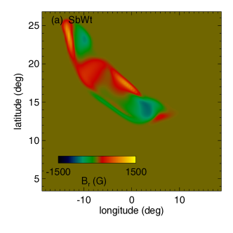
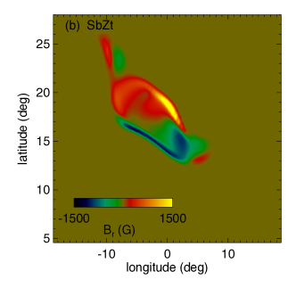
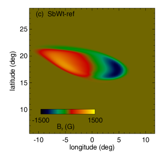
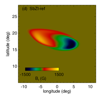
Figure 15: The normal flux distribution produced by the top of the rising tube approaching the upper boundary on a constant $r$ surface at $r=0.957R_{s}$, for the cases SbWt (a), SbZt (b), SbWt-ref (c), and SbZt-ref (d). Note in these plots, we have shifted the longitude of the apex location of the rising flux to 0 degree longitude.

In all the cases, the apex rises nearly radially, with a small poleward drift. Figure 15 shows the normal flux distribution produced by the emerging apex portion near the top boundary on a constant $r$ surface at $r=0.957R_{s}$. It can be seen that for all of the four cases the latitude of emergence is centered at a location just slightly poleward (by no more than about $3.5^{\circ}$) than the initial latitude of $15^{\circ}$. For the cases without convection (panels (c) and (d)), the apex portion produces a simple bipolar structure with a tilt angle of $7.2^{\circ}$ clockwise for the weakly twisted (SbWt-ref) case, and $16^{\circ}$ clockwise for the untwisted (SbZt-ref) case. These tilts are consistent with the mean tilt of solar active regions as described by Joy’s law. With convection, the additional distortion and undulation caused by the convective flows produce a more complex emergence pattern with multiple bipolar structures in the SbWt and SbZt cases as shown in Figures 15a and 15b. However, the leading (negative) polarity flux is on average equatorward and westward of the following (positive) polarity, consistent with the direction of the active region mean tilt. The tilt angle as determined by the flux weighted positions of the leading and following polarity flux concentrations is $29.2^{\circ}$ clockwise for the weakly twisted (SbWt) case and $53.2^{\circ}$ clockwise for the untwisted (SbZt) case, which are of the right sign but are of a significantly greater magnitude than the active region mean tilt.

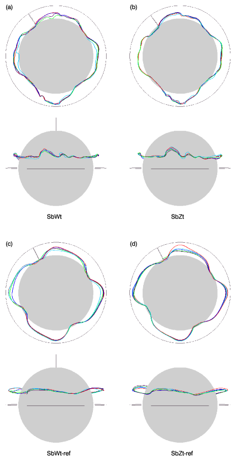
Figure 16: Polar and equatorial views of selected field lines in the rising flux tubes for the cases SbWt (a), SbZt (b), SbWt-ref (c), and SbZt-ref (d). For each of the cases, the polar (equatorial) view is the upper (lower) panel

Figure 16 shows 3D views of a few selected field lines traced from the apex portion in the rising flux tubes for the four cases: (a) SbWt, (b) SbZt, (c) SbWt-ref, and (d) SbZt-ref, as viewed from the pole (upper panel in each case), and from the equator (lower panel in each case). For all the cases, the apex of the rising tube is at the 6 o’clock location in the polar view and at the central meridian in the equatorial view. It can be seen that the field lines at the apex are pointing southeast-ward, i.e. consistent with the sense of tilts of solar active regions. The tilt angles of the field orientation from the east-west direction are significantly bigger in the convective cases (SbWt and SbZt in Figures 16a and 16b) compared to the non-convective reference cases (SbWt-ref and SbZt-ref in Figures 16c and 16d). In these particular convective cases, the convective flows have driven additional clock-wise rotation of the fields at the rising apex. A statistical study with many more simulations of rising flux tubes, sampling different times and locations of the convective flows (as was done with the thin flux tube model in Weber et al. (e.g. 2012)) are needed to determine whether the tilt angles at the apex of the emerging flux obey Joy’s law for solar active regions. Our initial simulations here show that even with a relatively strong initial magnetic field of 100 kG, a solar-like giant cell convection can significantly reshape the buoyantly rising loops and shorten the time for the apex to reach the top.

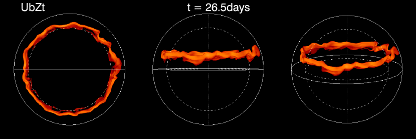
Figure 17: 3D volume rendering of the absolute magnetic field strength of the rising flux tube developed from the UbZt simulation as the apex at the right is reaching the top boundary. An MPEG animation of the evolution is available in the online version.

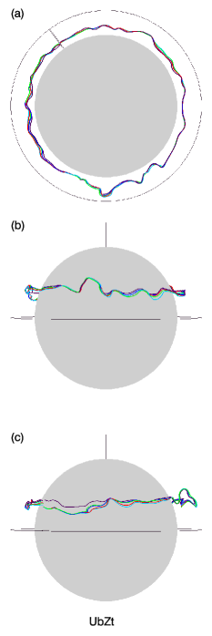
Figure 18: Selected field lines in the rising flux tube for the case UbZt as viewed from the pole with the apex located at the 6 o’clock position (a), and viewed from the equator with the apex located at the central meridian (b) and west limb (c) respectively.

We have also run a simulation (case UbZt) where the initial toroidal flux tube is uniformly buoyant along the tube with the magnetic buoyancy, such that the flux tube would have risen axisymmetrically under its buoyancy had it not been for the effect of the convective flows. Thus the development of undulations or loop structures is due entirely to the convective flows. Figure 17 shows 3D volume rendering of the absolute magnetic field strength of the rising loops that develop, as viewed from 3 different perspectives, with the apex portion approaching the top boundary located at the right in all three views. An MPEG movie of the evolution of the rising flux tube viewed from the same perspectives is available in the online version. We see that loops with shorter footpoint separations form compared to the 4 major loops formed in the SbZt case. A set of selected field lines traced from the apex portion approaching the top are also shown in a polar view (Figure 18a) with the apex positioned at the 6 o’clock location, and two equatorial views (Figures 18b and 18c) with the apex positioned at the central meridian and at the west limb respectively. We can see that despite the fact that the initial buoyancy is uniform along the tube, the convective downdrafts are able to hold back portions of the buoyant tube and lead to the formation of loop structures with undulations that span up to 70% of the depth of the convection zone (based on the apex and troughs of the field lines) in a time scale of about a month. However, the troughs of the loops are not as deeply rooted as the major loops formed in the SbZt case (compare Figure 18a with the top panel of Figure 16b). All of the troughs are above the initial depth of the toroidal tube, meaning that the downdrafts are not able to completely overcome the magnetic buoyancy. Similar to the SbZt case, the convective flows have driven a significantly larger clockwise tilt from the east-west direction at the apex of the emerging loop, as can be seen in the field line orientation at the central meridian in Figure 18b. of the emerging loop

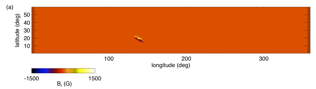
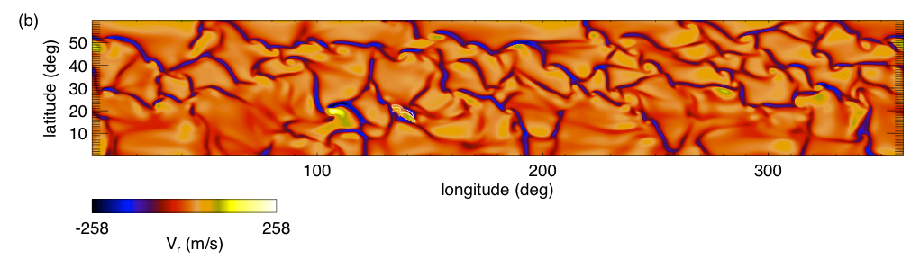
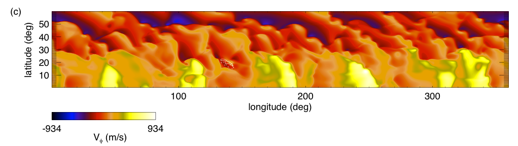
Figure 19: Constant $r$ slices of $B_{r}$ (a), $v_{r}$ (b) and $v_{\phi}$ (c) at $r=0.957R_{s}$ (about 30 Mm below the top boundary) at the time when the the apex portion of the rising tube is reaching the top boundary for the UbZt case. White contours in (b) and (c) are contours of $B_{r}$ outlining the positive (solid line) and negative (dashed line) magnetic flux concentrations.

Figure 19 shows the normal flux distribution $B_{r}$, radial velocity $v_{r}$, and zonal flow $v_{\phi}$ on a constant $r$ slice at $r=0.957R_{s}$, about 30 Mm below the top boundary, at the time when the apex portion of the rising flux tube approaches the top boundary for the UbZt case. An emerging region with a large overall tilt ($75.4^{\circ}$ clockwise based on the flux weighted positions of the leading and following polarity flux concentrations) of the correct sign has formed by the apex of the rising tube. The region of emerging flux corresponds to a local region of upflow (with speed reaching about 100 m/s) surrounded by narrow downflow lanes (see Figure 19b). The emerging flux also shows a retrograde zonal flow (peaks at about -200 m/s) in the midst of the prograde flows of the banana cells (see Figure 19c). It corresponds to the most retrograde portion of plasma at that latitude. Relative to the mean plasma zonal flow speed at that latitude (about 225 m/s), the emerging flux region has a relative (flux weighted) mean speed of -348 m/s. Similar results on the relative speeds of the emerging flux region are found for the SbWt and SbZt cases.

5 Discussions

We have used a finite-difference based spherical anelastic MHD code (FSAM) to simulate rotating solar convection and the buoyant rise of super-equipartition field strength flux tubes through the convective envelope in the presence of the giant-cell convection and the associated mean flows. We achieved a statistically steady solution of giant-cell convection with a solar-like differential rotation using a relatively low viscosity $\nu=10^{12}\,{\rm cm}^{2}\,{\rm s}^{-1}$, but a high value of thermal diffusion $K=2\times 10^{13}\,{\rm cm}^{2}\,{\rm s}^{-1}$. The high thermal diffusion allows most of the solar luminosity to be carried via thermal conduction, so that the resolved giant-cell convection flow speed is not too high and the convection remains sufficiently rotationally constrained to give a solar-like differential rotation with the right amplitude. Into the giant-cell convection near the bottom of the convective envelope, we insert toroidal flux tubes of 100 kG field strength and with different forms of magnetic buoyancy distribution to model their rise through the convective envelope in the presence of convection. We simulate the rise of the flux tube with no explicit magnetic diffusion $\eta$ and a quenching of thermal diffusion $K$ in the flux tube to best preserve the magnetic buoyancy of the initial flux tube.

The simulations show that with a strong, super-equipartition field strength of 100 kG, magnetic buoyancy dominates the rise but the strong down-flows can significantly modify the shape of the $\Omega$-shaped emerging loops, and substantially reduce the rise time for the apex to reach the top boundary. Even if the initial tube is uniformly buoyant, it is found that convection can produce loop structures with undulations that extend most of the depth of the CZ in a time scale of about a month. For the weakly twisted and (initially) untwisted cases we simulated, the apex portion rises nearly radially and produces an emerging region with an overall tilt angle consistent with the active region tilts, although there is continued and substantial loss of flux during the rise. Thus it appears that the current simulations suggest that a significant twist in the toroidal magnetic fields in the bottom of the convection zone is not required for the emergence of coherent active regions. We emphasize that the current simulations are in a rather laminar region with the Reynolds number for the rising tube estimated to be $\sim 10$. This would limit the formation of small scale structures and improve the cohesion of the rising flux. However there is difficulty to significantly reduce the viscosity if one wants to also self-consistently maintain a solar-like differential rotation (e.g. Featherstone & Miesch, 2012). On the other hand, the ubiquitous presence of small scale magnetic fields in a convective dynamo in the CZ may suppress the development of small scale flows via the magnetic stresses, effectively increasing the viscosity (Longcope et al., 2003), and allow a solar like differential rotation to be maintained at a substantially lower fluid viscosity (Fan 2013 in preparation). Thus the presence of the ambient small scale magnetic field may effectively improve the cohesion of the strong buoyant flux tubes with weak twists, which is indicated in the recent convective dynamo simulations in faster rotating convective envelopes by Nelson et al. (2013b). Clearly 3D convective dynamo simulations in the solar convective envelope that model both the generation of the dynamo mean field and the self-consistent formation and rise of active region flux in the midst of small scale fields are needed to obtain a complete understanding of the solar cycle dynamo and active region formation.

Appendix A The Numerical Algorthms of FSAM

In this Appendix we describe how FSAM numerically solves equations (16), (20), (22), and (5), to advance the dependent variables ${\bf v}$, $p_{1}$, $s_{1}$, and ${\bf B}$. FSAM uses a staggered spatial discretization as described in Stone & Norman (1992a), where the vector quantities ${\bf v}$ and ${\bf B}$ are defined on the faces of each finite-volume cell of the grid, scalar quantities $p_{1}$, $s_{1}$, $T_{1}$, are defined at the center of each finite-volume cell, and the ${\bf v}\times{\bf B}$ electric field and the current density $\nabla\times{\bf B}$ in the induction equation are defined on the cell edges.

First we define some notations to be used frequently in the rest of the Appendix. For the spherical polar coordinate system used by this code, we use subscript $m=1,2,3$ to denote respectively the $r$, $\theta$, $\phi$ direction or component, i.e. we have $(x_{1},x_{2},x_{3})=(r,\theta,\phi)$, $(v_{1},v_{2},v_{3})=(v_{r},v_{\theta},v_{\phi})$, $(B_{1},B_{2},B_{3})=(B_{r},B_{\theta},B_{\phi})$. Also we make use of the following coordinate scaling coefficients defined as: $g_{2}=r$, $g_{31}=r$, and $g_{32}=\sin\theta$ (notations used in Stone & Norman (1992a)). Consider in general a row of cells in the $m$-direction ($m=1,2,3$), whose centers’ $x_{m}$ coordinates are located at $x_{m,i}$, $i=1,2,3,...$, and whose cell averaged $Q$ values are denoted by $Q_{i}$. For evaluating the various fluxes at the cell face located at $x_{m,i-1/2}$ between the two adjacent cells centered on $x_{m,i-1}$ and $x_{m,i}$, we define

$$\delta_{m}Q\equiv Q_{i}-Q_{i-1}$$ (A1)

to be the simple finite difference between the two adjacent cells (in the m-direction), and we will use $Q^{L}$ and $Q^{R}$ to denote the ‘left’ and ‘right’ $Q$ values on the cell face, evaluated through a certain reconstruction of the $Q$ profile within the cell to the left and right of the cell face, respectively. Specifically, the assumed profile $Q(x_{m})$ within the cell centered on $x_{m,i}$ is given by a linear reconstruction with a $minmod$ slope limiter:

$$Q(x_{m})=Q_{i}+s_{m,i}(x_{m}-x_{m,i}),$$ (A2)

where $s_{m,i}$ is a limited slope (in the m-direction) for the cell given by

$$s_{m,i}=minmod\left({Q_{i+1}-Q_{i}\over x_{m,i+1}-x_{m,i}},{Q_{i}-Q_{i-1}\over x_{m,i}-x_{m,i-1}}\right)$$ (A3)

and the $minmod$ function is defined as

$$minmod(y1,y2)\equiv sgn(y1)\max[0,\min(y1,sgn(y1)y2)].$$ (A4)

Thus the right and left values, $Q^{R}$ and $Q^{L}$, for the cell face located at $x_{m,i-1/2}$, between the two neighboring cells centered at $x_{m,i-1}$ and $x_{m,i}$ are:

$$Q^{L}=Q_{i-1}+s_{m,i-1}(x_{m,i-1/2}-x_{m,i-1}),$$ (A5)

$$Q^{R}=Q_{i}-s_{m,i}(x_{m,i}-x_{m,i-1/2}),$$ (A6)

and we let

$$\Delta_{m}Q\equiv Q^{R}-Q^{L},$$ (A7)

denoting the limited difference between the right and left states at the cell face at $x_{m,i-1/2}$, and

$$<\!Q\!>_{m}={Q^{R}+Q^{L}\over 2}$$ (A8)

denoting the mean of the left, right values of $Q$ evaluated at the cell face at $x_{m,i-1/2}$.

The 1,2,3-components of the momentum equation (16), and the entropy equation (22) we solve written explicitly in spherical coordinates are:

$${\partial\over\partial t}(\rho_{0}v_{1}) = -{1\over g_{2}g_{31}}{\partial\over\partial x_{1}}\left[g_{2}g_{31}\left(\rho_{0}v_{1}v_{1}\right)^{*}\right]$$ (A9)

$$-{1\over g_{2}g_{32}}{\partial\over\partial x_{2}}\left[g_{32}\left(\rho_{0}v_{2}v_{1}\right)^{*}\right]$$

$$-{1\over g_{31}g_{32}}{\partial\over\partial x_{3}}\left(\rho_{0}v_{3}v_{1}\right)^{*}$$

$$+\frac{1}{g_{2}g_{32}}\frac{\partial}{\partial x_{2}}(g_{32}B_{1}B_{2})+\frac{1}{g_{31}g_{32}}\frac{\partial}{\partial x_{3}}(B_{1}B_{3})+\frac{1}{{g_{2}}^{2}{g_{31}}^{2}}\frac{\partial}{\partial x_{1}}\left({g_{2}}^{2}{g_{31}}^{2}\frac{{B_{1}}^{2}}{2}\right)$$

$$-\frac{1}{{g_{31}}^{2}}\frac{\partial}{\partial x_{1}}\left(\frac{{g_{31}}^{2}{B_{3}}^{2}}{2}\right)-\frac{1}{{g_{2}}^{2}}\frac{\partial}{\partial x_{1}}\left(\frac{{g_{2}}^{2}{B_{2}}^{2}}{2}\right)$$

$$+\rho_{0}g_{0}\frac{s_{1}}{c_{p}}-\rho_{0}{\partial\over\partial x_{1}}\left({p_{1}\over\rho_{0}}\right)$$

$$+\rho_{0}v_{2}^{2}{1\over g_{2}}{\partial g_{2}\over\partial x_{1}}+\rho_{0}v_{3}^{2}{1\over g_{31}}{\partial g_{31}\over\partial x_{1}}+2\Omega\rho_{0}v_{3}\sin\theta$$

$$+\left[{1\over g_{2}g_{31}}{\partial\over\partial x_{1}}\left(g_{2}g_{31}\rho_{0}\nu S_{11}\right)+{1\over g_{2}g_{32}}{\partial\over\partial x_{2}}\left(g_{32}\rho_{0}\nu S_{12}\right)+{1\over g_{31}g_{32}}{\partial\over\partial x_{3}}\left(\rho_{0}\nu S_{13}\right)\right]$$

$$-\rho_{0}\nu S_{22}{1\over g_{2}}{\partial g_{2}\over\partial x_{1}}-\rho_{0}\nu S_{33}{1\over g_{31}}{\partial g_{31}\over\partial x_{1}}-{2\over 3}{\partial\over\partial x_{1}}\left(\rho_{0}\nu\nabla\cdot{\bf v}\right),$$

$${\partial\over\partial t}(\rho_{0}v_{2}) = -{1\over g_{2}g_{2}g_{31}}{\partial\over\partial x_{1}}\left[g_{2}g_{31}g_{2}^{2}\left(\rho_{0}v_{1}{v_{2}\over g_{2}}\right)^{*}\right]$$

$$-{1\over g_{2}g_{2}g_{32}}{\partial\over\partial x_{2}}\left[g_{32}g_{2}^{2}\left(\rho_{0}v_{2}{v_{2}\over g_{2}}\right)^{*}\right]$$

$$-{1\over g_{2}g_{31}g_{32}}{\partial\over\partial x_{3}}\left[g_{2}^{2}\left(\rho_{0}v_{3}{v_{2}\over g_{2}}\right)^{*}\right]$$

$$+\frac{1}{{g_{2}}^{2}g_{31}}\frac{\partial}{\partial x_{1}}({g_{2}}^{2}g_{31}B_{2}B_{1})+\frac{1}{g_{2}{g_{32}}^{2}}\frac{\partial}{\partial x_{2}}\left(\frac{{g_{32}}^{2}{B_{2}}^{2}}{2}\right)$$

$$+\frac{1}{g_{31}g_{32}}\frac{\partial}{\partial x_{3}}(B_{2}B_{3})-\frac{1}{g_{2}}\frac{\partial}{\partial x_{2}}\left(\frac{{B_{1}}^{2}}{2}\right)-\frac{1}{{g_{32}}^{2}g_{2}}\frac{\partial}{\partial x_{2}}\left(\frac{{g_{32}}^{2}{B_{3}}^{2}}{2}\right)$$

$$-{\rho_{0}\over g_{2}}{\partial\over\partial x_{2}}\left({p_{1}\over\rho_{0}}\right)$$

$$+\rho_{0}v_{3}^{2}{1\over g_{32}g_{2}}{\partial g_{32}\over\partial x_{2}}+{2\Omega}\rho_{0}v_{3}\cos\theta$$

$$+\left[{1\over g_{2}g_{31}}{\partial\over\partial x_{1}}\left(g_{2}g_{31}\rho_{0}\nu S_{21}\right)+{1\over g_{2}g_{32}}{\partial\over\partial x_{2}}\left(g_{32}\rho_{0}\nu S_{22}\right)+{1\over g_{31}g_{32}}{\partial\over\partial x_{3}}\left(\rho_{0}\nu S_{23}\right)\right]$$

$$+{\rho_{0}\nu}S_{21}{1\over g_{2}}{\partial g_{2}\over\partial x_{1}}-{\rho_{0}\nu}S_{33}{1\over g_{2}g_{32}}{\partial g_{32}\over\partial x_{2}}-{2\over 3}{1\over g_{2}}{\partial\over\partial x_{2}}\left(\rho_{0}\nu\nabla\cdot{\bf v}\right),$$

$${\partial\over\partial t}(\rho_{0}v_{3}) = -{1\over g_{31}g_{32}g_{2}g_{31}}{\partial\over\partial x_{1}}\left[g_{2}g_{31}g_{31}^{2}g_{32}^{2}\left(\left(\rho_{0}v_{1}{v_{3}\over g_{31}g_{32}}\right)^{*}+\rho_{0}v_{1}\Omega\right)\right]$$ (A11)

$$-{1\over g_{31}g_{32}g_{2}g_{32}}{\partial\over\partial x_{2}}\left[g_{32}g_{31}^{2}g_{32}^{2}\left(\left(\rho_{0}v_{2}{v_{3}\over g_{31}g_{32}}\right)^{*}+\rho_{0}v_{2}\Omega\right)\right]$$

$$-{1\over g_{31}g_{32}g_{31}g_{32}}{\partial\over\partial x_{3}}\left[g_{31}^{2}g_{32}^{2}\left(\left(\rho_{0}v_{3}{v_{3}\over g_{31}g_{32}}\right)^{*}+\rho_{0}v_{3}\Omega\right)\right]$$

$$+\frac{1}{g_{31}g_{32}g_{2}g_{31}}\frac{\partial}{\partial x_{1}}\left(g_{2}g_{31}g_{31}g_{32}B_{3}B_{1}\right)+\frac{1}{g_{31}g_{32}g_{2}g_{32}}\frac{\partial}{\partial x_{2}}\left(g_{32}g_{31}g_{32}B_{3}B_{2}\right)$$

$$+\frac{1}{g_{31}g_{32}}\frac{\partial}{\partial x_{3}}\left(\frac{{B_{3}}^{2}}{2}\right)-\frac{1}{g_{31}g_{32}}\frac{\partial}{\partial x_{3}}\left(\frac{{B_{2}}^{2}}{2}\right)-\frac{1}{g_{31}g_{32}}\frac{\partial}{\partial x_{3}}\left(\frac{{B_{1}}^{2}}{2}\right)$$

$$-{\rho_{0}\over g_{31}g_{32}}{\partial\over\partial x_{3}}\left({p_{1}\over\rho_{0}}\right)$$

$$+\left[{1\over g_{31}g_{32}g_{2}g_{31}}{\partial\over\partial x_{1}}\left(g_{2}g_{31}g_{31}g_{32}\rho_{0}\nu S_{31}\right)+{1\over g_{31}g_{32}g_{2}g_{32}}{\partial\over\partial x_{2}}\left(g_{32}g_{31}g_{32}\rho_{0}\nu S_{32}\right)\right.$$

$$\left.+{1\over g_{31}g_{32}}{\partial\over\partial x_{3}}\left(\rho_{0}\nu S_{33}\right)\right]-{2\over 3}{1\over g_{31}g_{32}}{\partial\over\partial x_{3}}\left(\rho_{0}\nu\nabla\cdot{\bf v}\right),$$

$$\rho_{0}T_{0}{\partial s_{1}\over\partial t} = -{1\over g_{2}g_{31}}{\partial\over\partial x_{1}}\left[g_{2}g_{31}\left(\rho_{0}T_{0}v_{1}(s_{1}+s_{0})\right)^{*}\right]$$ (A12)

$$-{1\over g_{2}g_{32}}{\partial\over\partial x_{2}}\left[g_{32}\left(\rho_{0}T_{0}v_{2}(s_{1}+s_{0})\right)^{*}\right]$$

$$-{1\over g_{31}g_{32}}{\partial\over\partial x_{3}}\left(\rho_{0}T_{0}v_{3}(s_{1}+s_{0})\right)^{*}$$

$$-\rho_{0}v_{1}(s_{1}+s_{0}){g_{0}\over c_{p}}$$

$$+\rho_{0}\nu(S_{12}^{2}+S_{23}^{2}+S_{31}^{2})+{1\over 6}\rho_{0}\nu\left[(S_{11}-S_{22})^{2}+(S_{22}-S_{33})^{2}+(S_{33}-S_{11})^{2}\right]$$

$$+Q_{\rm num}+\eta(\nabla\times{\bf B})^{2}+\nabla\cdot\left(K\rho_{0}T_{0}\nabla s_{1}\right)$$

$$+\nabla\cdot\left({16\sigma_{s}T_{0}^{3}\over 3\kappa\rho_{0}}\nabla T_{0}\right),$$

where

$$S_{11}=2{\partial v_{1}\over\partial x_{1}},$$ (A13)

$$S_{22}={2\over g_{2}}{\partial v_{2}\over\partial x_{2}}+{2v_{1}\over g_{2}}{\partial g_{2}\over\partial x_{1}}$$ (A14)

$$S_{33}={2\over g_{31}g_{32}}{\partial v_{3}\over\partial x_{3}}+{2v_{1}\over g_{31}}{\partial g_{31}\over\partial x_{1}}+{2v_{2}\over g_{2}g_{32}}{\partial g_{32}\over\partial x_{2}}$$ (A15)

$$S_{12}=S_{21}={1\over g_{2}}{\partial v_{1}\over\partial x_{2}}+g_{2}{\partial\over\partial x_{1}}\left({v_{2}\over g_{2}}\right)$$ (A16)

$$S_{23}=S_{32}={1\over g_{31}g_{32}}{\partial v_{2}\over x_{3}}+{g_{32}\over g_{2}}{\partial\over\partial x_{2}}\left({v_{3}\over g_{32}}\right)$$ (A17)

$$S_{31}=S_{13}={1\over g_{31}g_{32}}{\partial v_{1}\over\partial x_{3}}+g_{31}{\partial\over\partial x_{1}}\left({v_{3}\over g_{31}}\right).$$ (A18)

Note that the 3-component of the momentum equation (A11) is written in the angular momentum conservative form.

For spatially discretizing equations (A9), (LABEL:eq:mom2), (A11), and (A12), standard 2nd order interpolations and finite-differences are applied to all the quantities and derivatives, except for the fluxes (with superscript ‘*’) in the first 3 advection terms on the right hand side (RHS) of each of the above equations. For evaluating these fluxes through their respective cell faces, we use a modified Lax-Friedrichs scheme (Rempel et al., 2009) to get an upwinded evaluation of the fluxes as follows.

For the first 3 terms on the RHS of equation (A9), the upwinded evaluation of the 1-, 2-, and 3-fluxes $\rho_{0}v_{1}v_{1}$, $\rho_{0}v_{2}v_{1}$, and $\rho_{0}v_{3}v_{1}$ through their respective cell-faces at respectively $x_{1}=x_{1,i-1/2}$, $x_{2}=x_{2,i-1/2}$, and $x_{3}=x_{3,i-1/2}$ are

$${\left(\rho_{0}v_{1}v_{1}\right)^{*}}_{i-1/2}=\left(\rho_{0}v_{1}\right)_{i-1/2}<\!\!v_{1}\!\!>_{1}-\left(\rho_{0}{|v_{1}|+c_{a}\,q_{1,v_{1}}^{l}\over 2}\right)_{i-1/2}\Delta_{1}v_{1},$$ (A19)

$${\left(\rho_{0}v_{2}v_{1}\right)^{*}}_{i-1/2}=\left(\rho_{0}v_{2}\right)_{i-1/2}<\!\!v_{1}\!\!>_{2}-\left(\rho_{0}{|v_{2}|+c_{a}\,q_{2,v_{1}}^{l}\over 2}\right)_{i-1/2}\Delta_{2}v_{1},$$ (A20)

$${\left(\rho_{0}v3v_{1}\right)^{*}}_{i-1/2}=\left(\rho_{0}v_{3}\right)_{i-1/2}<\!\!v_{1}\!\!>_{3}-\left(\rho_{0}{|v_{3}|+c_{a}\,q_{3,v_{1}}^{l}\over 2}\right)_{i-1/2},\Delta_{3}v_{1},$$ (A21)

where $<\!\!v_{1}\!\!>_{1}$, $<\!\!v_{1}\!\!>_{2}$, $<\!\!v_{1}\!\!>_{3}$ correspond to the left-right averages at the respective cell-faces as given by equation (A8), and $\Delta_{1}v_{1}$, $\Delta_{2}v_{1}$, $\Delta_{3}v_{1}$ correspond to the limited differences evaluated at the respective cell-faces as given by equation (A7), and

$$q_{m,v_{1}}={\Delta_{m}v_{1}\over\delta_{m}v_{1}},$$ (A22)

with $m=1,2,3$, and $\delta_{m}v_{1}$ given by equation (A1). Also on the RHS of equations (A19), (A20), (A21), all the other quantities in $()$ are evaluated via standard 2nd order interpolation at the cell-faces, and $c_{a}$ denotes the Alfvén speed and $l=4$. The 2nd terms on the RHS of equations (A19), (A20), and (A21) correspond to a diffusive flux resulting from the upwinded evaluation (Rempel et al., 2009). It can be seen that the speed $c_{a}$ in the diffusive flux is scale by the smoothness factor $q_{m,v_{1}}$ (given by equation [A22]) to the $l$th power. It can be shown that the limited difference $\Delta_{m}v_{1}$ is always of the same sign and of a smaller magnitude compared to the simple finite difference $\delta_{m}v_{1}$. The factor $q_{m,v_{1}}^{l}\ll 1$ when the variation of $v_{1}$ in the $m$-direction is smooth, and thus reduces the speed in the diffusive flux.

In the same way, for equation (LABEL:eq:mom2), the upwinded 1-, 2-, and 3-fluxes $\rho_{0}v_{1}(v_{2}/g_{2})$, $\rho_{0}v_{2}(v_{2}/g_{2})$, and $\rho_{0}v_{3}(v_{2}/g_{2})$ through their respective cell-faces are:

$${\left(\rho_{0}v_{1}{v_{2}\over g_{2}}\right)^{*}}_{i-1/2}=\left(\rho_{0}v_{1}\right)_{i-1/2}<\!\!{v_{2}\over g_{2}}\!\!>_{1}-\left(\rho_{0}{|v_{1}|+c_{a}\,q_{1,v_{2}}^{l}\over 2}\right)_{i-1/2}\Delta_{1}\left({v_{2}\over g_{2}}\right)$$ (A23)

$${\left(\rho_{0}v_{2}{v_{2}\over g_{2}}\right)^{*}}_{i-1/2}=\left(\rho_{0}v_{2}\right)_{i-1/2}<\!\!{v_{2}\over g_{2}}\!\!>_{2}-\left(\rho_{0}{|v_{2}|+c_{a}\,q_{2,v_{2}}^{l}\over 2}\right)_{i-1/2}\Delta_{2}\left({v_{2}\over g_{2}}\right)$$ (A24)

$${\left(\rho_{0}v_{3}{v_{2}\over g_{2}}\right)^{*}}_{i-1/2}=\left(\rho_{0}v_{3}\right)_{i-1/2}<\!\!{v_{2}\over g_{2}}\!\!>_{3}-\left(\rho_{0}{|v_{3}|+c_{a}\,q_{3,v_{2}}^{l}\over 2}\right)_{i-1/2}\Delta_{3}\left({v_{2}\over g_{2}}\right),$$ (A25)

where

$$q_{m,v_{2}}={\Delta_{m}(v_{2}/g_{2})\over\delta_{m}(v_{2}/g_{2})},$$ (A26)

for equation (A11), the upwinded 1-, 2-, and 3-fluxes $\rho_{0}v_{1}(v_{3}/g_{31}g_{32})$, $\rho_{0}v_{2}(v_{3}/g_{31}g_{32})$, and $\rho_{0}v_{3}(v_{3}/g_{31}g_{32})$ through their respective cell-faces are:

$${\left(\rho_{0}v_{1}{v_{3}\over g_{31}g_{32}}\right)^{*}}_{i-1/2}=\left(\rho_{0}v_{1}\right)_{i-1/2}<\!\!{v_{3}\over g_{31}g_{32}}\!\!>_{1}-\left(\rho_{0}{|v_{1}|+c_{a}\,q_{1,v_{3}}^{l}\over 2}\right)_{i-1/2}\Delta_{1}\left({v_{3}\over g_{31}g_{32}}\right)$$ (A27)

$${\left(\rho_{0}v_{2}{v_{3}\over g_{31}g_{32}}\right)^{*}}_{i-1/2}=\left(\rho_{0}v_{2}\right)_{i-1/2}<\!\!{v_{3}\over g_{31}g_{32}}\!\!>_{2}-\left(\rho_{0}{|v_{2}|+c_{a}\,q_{2,v_{3}}^{l}\over 2}\right)_{i-1/2}\Delta_{2}\left({v_{3}\over g_{31}g_{32}}\right)$$ (A28)

$${\left(\rho_{0}v_{3}{v_{3}\over g_{31}g_{32}}\right)^{*}}_{i-1/2} = \left(\rho_{0}v_{3}\right)_{i-1/2}<\!\!{v_{3}\over g_{31}g_{32}}\!\!>_{3}$$ (A29)

$$-\left(\rho_{0}{|v_{3}|+c_{a}\,q_{3,v_{3}}^{l}\over 2}\right)_{i-1/2}\Delta_{3}\left({v_{3}\over g_{31}g_{32}}\right),$$

where

$$q_{m,v_{3}}={\Delta_{m}(v_{3}/g_{31}g_{32})\over\delta_{m}(v_{3}/g_{31}g_{32})},$$ (A30)

and finally for equation (A12), the upwinded 1-, 2-, and 3-fluxes $\rho_{0}T_{0}v_{1}(s_{1}+s_{0})$, $\rho_{0}T_{0}v_{2}(s_{1}+s_{0})$, and $\rho_{0}T_{0}v_{3}(s_{1}+s_{0})$ through their respective cell-faces are:

$${\left(\rho_{0}T_{0}v_{1}(s_{1}+s_{0})\right)^{*}}_{i-1/2} = \left(\rho_{0}T_{0}v_{1}\right)_{i-1/2}<\!\!s_{1}+s_{0}\!\!>_{1}$$ (A31)

$$-\left(\rho_{0}T_{0}{|v_{1}|+c_{a}\,q_{1,s}^{l}\over 2}\right)_{i-1/2}\Delta_{1}\left(s_{1}+s_{0}\right),$$

$${\left(\rho_{0}T_{0}v_{2}(s_{1}+s_{0})\right)^{*}}_{i-1/2} = \left(\rho_{0}T_{0}v_{2}\right)_{i-1/2}<\!\!s_{1}+s_{0}\!\!>_{2}$$ (A32)

$$-\left(\rho_{0}T_{0}{|v_{2}|+c_{a}\,q_{2,s}^{l}\over 2}\right)_{i-1/2}\Delta_{2}\left(s_{1}+s_{0}\right),$$

$${\left(\rho_{0}T_{0}v_{3}(s_{1}+s_{0})\right)^{*}}_{i-1/2} = \left(\rho_{0}T_{0}v_{3}\right)_{i-1/2}<\!\!s_{1}+s_{0}\!\!>_{3}$$ (A33)

$$-\left(\rho_{0}T_{0}{|v_{3}|+c_{a}\,q_{3,s}^{l}\over 2}\right)_{i-1/2}\Delta_{3}\left(s_{1}+s_{0}\right),$$

where

$$q_{m,s}={\Delta_{m}(s_{1}+s_{0})\over\delta_{m}(s_{1}+s_{0})}.$$ (A34)

Furthermore, in the RHS of the entropy equation (A12) we have also included a numerical heating term $Q_{\rm num}$ that corresponds to the dissipation of kinetic energy due to the diffusive fluxes (the 2nd term in the RHS of eqs. [A19], [A20], [A21], [A23], [A24], [A25], [A27], [A28], [A29]), by taking the dot product of the diffusive fluxes with the appropriate velocity gradients (computed via the standard centered finite difference),

$$Q_{\rm num} = \left(\rho_{0}{|v_{1}|+c_{a}\,q_{1,v_{1}}^{l}\over 2}\,\Delta_{1}v_{1}\right){\partial v_{1}\over\partial x_{1}}+\left(\rho_{0}{|v_{2}|+c_{a}\,q_{2,v1}^{l}\over 2}\,\Delta_{2}v_{1}\right){1\over g_{2}}{\partial v_{1}\over\partial x_{2}}$$ (A35)

$$+\left(\rho_{0}{|v_{3}|+c_{a}\,q_{3,v1}^{l}\over 2}\,\Delta_{3}v_{1}\right){1\over g_{31}g_{32}}{\partial v_{1}\over\partial x_{3}}+\left(\rho_{0}{|v_{1}|+c_{a}\,q_{1,v_{2}}^{l}\over 2}g_{2}^{2}\,\Delta_{1}\left({v_{2}\over g_{2}}\right)\right){\partial\over\partial x_{1}}\left({v_{2}\over g_{2}}\right)$$

$$+\left(\rho_{0}{|v_{2}|+c_{a}\,q_{2,v_{2}}^{l}\over 2}g_{2}^{2}\,\Delta_{2}\left({v_{2}\over g_{2}}\right)\right){1\over g_{2}}{\partial\over\partial x_{2}}\left({v_{2}\over g_{2}}\right)$$

$$+\left(\rho_{0}{|v_{3}|+c_{a}\,q_{3,v_{2}}^{l}\over 2}g_{2}^{2}\,\Delta_{3}\left({v_{2}\over g_{2}}\right)\right){1\over g_{31}g_{32}}{\partial\over\partial x_{3}}\left({v_{2}\over g_{2}}\right)$$

$$+\left(\rho_{0}{|v_{1}|+c_{a}\,q_{1,v_{3}}^{l}\over 2}g_{31}^{2}g_{32}^{2}\,\Delta_{1}\left({v_{3}\over g_{31}g_{32}}\right)\right){\partial\over\partial x_{1}}\left({v_{3}\over g_{31}g_{32}}\right)$$

$$+\left(\rho_{0}{|v_{2}|+c_{a}\,q_{2,v_{3}}^{l}\over 2}g_{31}^{2}g_{32}^{2}\,\Delta_{2}\left({v_{3}\over g_{31}g_{32}}\right)\right){1\over g_{2}}{\partial\over\partial x_{2}}\left({v_{3}\over g_{31}g_{32}}\right)$$

$$+\left(\rho_{0}{|v_{3}|+c_{a}\,q_{3,v_{3}}^{l}\over 2}g_{31}^{2}g_{32}^{2}\,\Delta_{3}\left({v_{3}\over g_{31}g_{32}}\right)\right){1\over g_{31}g_{32}}{\partial\over\partial x_{3}}\left({v_{3}\over g_{31}g_{32}}\right),$$

and then interpolating to the cell centers where $s_{1}$ is defined.

The pressure equation (20) we solve can be rewritten as:

$${1\over\rho_{0}}{\partial\over\partial x_{1}}\left(g_{2}g_{31}\rho_{0}{\partial P\over\partial x_{1}}\right)+{1\over g_{32}}{\partial\over\partial x_{2}}\left(g_{32}{\partial P\over\partial x_{2}}\right)+{1\over g_{32}^{2}}{\partial^{2}P\over\partial x_{3}^{2}}$$ (A36)

$$= {g_{2}^{2}\over\rho_{0}}\nabla\cdot{\cal F},$$

where $P\equiv p_{1}/\rho_{0}$. This linear equation is solved as follows. The 3-direction ($\phi$-direction) is periodic (for a full $2\pi$ azimuth), so we carry out a Fourier decomposition of $P$ in the $x_{3}$-dimension such that:

$$P_{k}\equiv P|_{x_{3}=x_{3,k}}=\sum_{n=0}^{N-1}{\hat{P}}_{n}e^{i2\pi f_{n}x_{3,k}}$$ (A37)

where $x_{3,k}$ with $k=1,2,...N$ are the $N$ uniformly spaced grid points in $x_{3}\in[0,2\pi]$, $f_{n}=n/2\pi$ with $n=0,1,...N-1$ denotes the discrete spatial frequency, and ${\hat{P}}_{n}$ denotes the amplitude of the Fourier component with frequency $f_{n}$. Then the centered finite difference evaluation of $\partial^{2}P/\partial x_{3}^{2}$ gives:

$$\left({\partial^{2}P\over\partial x_{3}^{2}}\right)_{k}=\frac{P_{k+1}-2P_{k}+P_{k-1}}{(\delta x_{3})^{2}}=\sum_{n=0}^{N-1}\left({2\cos(2\pi n/N)-2\over(\delta x_{3})^{2}}\right){\hat{P}}_{n}e^{i2\pi f_{n}x_{3,k}},$$ (A38)

and equation (A36) leads to the following 2D separable linear equation for the Fourier component ${\hat{P}_{n}}(x_{1},x_{2})$:

$${1\over\rho_{0}}{\partial\over\partial x_{1}}\left(g_{2}g_{31}\rho_{0}{\partial{\hat{P}}_{n}\over\partial x_{1}}\right)+{1\over g_{32}}{\partial\over\partial x_{2}}\left(g_{32}{\partial{\hat{P}}_{n}\over\partial x_{2}}\right)-{1\over g_{32}^{2}}\left({2-2\cos(2\pi n/N)\over(\delta x_{3})^{2}}\right){\hat{P}}_{n}$$ (A39)

$$= {\hat{R}}_{n},$$

where $\delta x_{3}$ denotes the grid spacing in $x_{3}$, and ${\hat{R}}_{n}$ is the Fourier transform of the RHS of equation (A36). Discretizing the above 2D linear equation leads to a block tridiagonal system, which is solved using the routine blktri.f in the FISHPACK math library of the National Center for Atmosphereic Research (NCAR), based on the generalized cyclic reduction scheme developed by P. Swatztrauber of NCAR.

For solving the induction equation (5) we use the constrained transport (CT) scheme on the staggered grid (Stone & Norman, 1992b) to ensure the divergence free condition for the magnetic field (eq. [4]) is satisfied to round-off errors. The CT scheme is used in conjuction with an upwinded evaluation of both ${\bf v}$ and ${\bf B}$ based on the Alfvén wave characteristics for computing the ${\bf v}\times{\bf B}$ electric field on the cell edges as described in Stone & Norman (1992b). The upwinded evaluation of the electric field would entail numerical dissipation of the magnetic field, which we did not put back as heating into the entropy equation. Thus, this is a cause of loss of conservation of total energy due to numerical dissipation in the code. We also evaluate the physical resistive electric field $\eta\nabla\times{\bf B}$ in equation (5) on the cell edges following the CT scheme, with the derivatives computed using simple second order finite differences. The Ohmic heating produced by the physical resistivity is being included in the entropy equation (A12).

After the RHS of all of the equations (A9), (LABEL:eq:mom2), (A11), and (A12) are evaluated at the appropriated cell locations as described above, we advance the equations in time using a simple second-order predictor-corrector time stepping. The linear elliptic pressure equation (A36) is solved at every sub-timestep to obtain $p_{1}$ needed for advancing equations (A9), (LABEL:eq:mom2), and (A11).

Figure 9: The final steady state entropy gradient reached by the rotating solar convective envelope in the convection simulation described in Section 4.1

Figure 10: Total heat flux due to convection ($H_{\rm conv}$) and conduction ($H_{\rm cond}$) through the convective envelope when the solution has reached a statistical steady state.

Figure 12: Peak downflow speed, peak upflow speed, and the RMS vertical flow speed of the convective flows in the solar convective envelope as a function of depth, averaged over 30 evenly spaced temporal samples over a period of about 3 months.

Table 1: Simulation Parameters for FSAM/ASH Comparison

Parameters	Values
ri	4.872$\times$1010 cm
ro	6.960$\times$1010 cm
$\rho_{i}$	0.36 g cm-3
$N_{\rho}$	1
n	1.5
cp	3.5$\times$108 erg g-1 K-1
Mint	1.989$\times$1033 g
$\Omega$	2.7$\times$10-6 s-1
$\nu$	7.74$\times$1012 cm2 s-1
$K$	7.74$\times$1012 cm2 s-1
$\Delta S$	1543.7 erg K-1 g-1

Table 2: Summary of the Rising Flux Tube Simulations

Label	Initial buoyancy	Twist rate $q\,\,\,(a^{-1})$	With convection?
SbWt-ref	Sinusoidal	-0.15	No
SbZt-ref	Sinusoidal	0.	No
SbWt	Sinusoidal	-0.15	Yes
SbZt	Sinusoidal	0.	Yes
UbZt	Uniform	0.	Yes

References

- Brun et al. (2004) Brun, A. S., Miesch, M. S., & Toomre, J. 2004, The Astrophysical Journal, 614, 1073
- Christensen-Dalsgaard et al. (1996) Christensen-Dalsgaard, J., Dappen, W., Ajukov, S. V., et al. 1996, Science, 272, 1286
- Elliott et al. (2000) Elliott, J. R., Miesch, M. S., & Toomre, J. 2000, ApJ, 533, 546
- Fan (2008) Fan, Y. 2008, ApJ, 676, 680
- Fan et al. (2003) Fan, Y., Abbett, W. P., & Fisher, G. H. 2003, ApJ, 582, 1206
- Featherstone et al. (2013) Featherstone, N., Brown, B., & Miesch, M. S. 2013, in preparation
- Featherstone & Miesch (2012) Featherstone, N., & Miesch, M. S. 2012, in American Astronomical Society Meeting Abstracts, Vol. 220, American Astronomical Society Meeting Abstracts #220, 123.01
- Gastine et al. (2012) Gastine, T., Wicht, J., & Aurnou, J. M. 2012, ArXiv e-prints
- Jones et al. (2011) Jones, C. A., Boronski, P., Brun, A. S., et al. 2011, Icarus, 216, 120
- Jouve & Brun (2009) Jouve, L., & Brun, A. S. 2009, ApJ, 701, 1300
- Jouve et al. (2013) Jouve, L., Brun, A. S., & Aulanier, G. 2013, ApJ, 762, 4
- Longcope et al. (2003) Longcope, D. W., McLeish, T. C. B., & Fisher, G. H. 2003, ApJ, 599, 661
- Miesch et al. (2008) Miesch, M. S., Brun, A. S., De Rosa, M. L., & Toomre, J. 2008, ApJ, 673, 557
- Miesch et al. (2006) Miesch, M. S., Brun, A. S., & Toomre, J. 2006, ApJ, 641, 618
- Nelson et al. (2011) Nelson, N. J., Brown, B. P., Brun, A. S., Miesch, M. S., & Toomre, J. 2011, ApJ, 739, L38
- Nelson et al. (2013a) —. 2013a, ApJ, 762, 73
- Nelson et al. (2013b) Nelson, N. J., Brown, B. P., Sacha Brun, A., Miesch, M. S., & Toomre, J. 2013b, Sol. Phys.
- Rempel et al. (2009) Rempel, M., Schüssler, M., & Knölker, M. 2009, ApJ, 691, 640
- Stone & Norman (1992a) Stone, J. M., & Norman, M. L. 1992a, ApJS, 80, 753
- Stone & Norman (1992b) —. 1992b, ApJS, 80, 791
- Weber et al. (2011) Weber, M. A., Fan, Y., & Miesch, M. S. 2011, ApJ, 741, 11
- Weber et al. (2012) —. 2012, Sol. Phys.