Bouncing cosmologies in massive gravity on de Sitter

Abstract

In the framework of massive gravity with a de Sitter reference metric, we study homogeneous and isotropic solutions with positive spatial curvature. Remarkably, we find that bounces can occur when cosmological matter satisfies the strong energy condition, in contrast to what happens in classical general relativity. This is due to the presence in the Friedmann equations of additional terms, which depend on the scale factor and its derivatives and can be interpreted as an effective fluid. We present a detailed study of the system using a phase space analysis. After having identified the fixed points of the system and investigated their stability properties, we discuss the cosmological evolution in the global physical phase space. We find that bouncing solutions are generic. Moreover, depending on the solutions, the cosmological evolution can lead to an asymptotic de Sitter regime, a curvature singularity or a determinant singularity.

I Introduction

After the recent discovery of a two-parameter class of massive gravity theories deRham:2010kj that are not plagued by the Bouldware-Deser ghost Boulware:1973my , there has been an intense activity to investigate the cosmological consequences of these models and of their extensions. In particular, it was shown that ghost-free massive gravity with Minkowski as fiducial metric does not admit spatially flat FLRW solutions D'Amico:2011jj , although it does admit open FLRW solutions Gumrukcuoglu:2011ew . Using a more general fiducial metric (which also leads to ghost-free massive gravity Hassan_etal ), one can find FLRW solutions of arbitrary spatial curvature. This applies to the interesting case of a de Sitter fiducial metric, which was studied in Fasiello:2012rw and Langlois:2012hk . Cosmological solutions have also been investigated in other works (see e.g. cosmo_sol ). Beyond the question of their existence, one should stress that the viability of cosmological solutions depends on their stability properties and most cosmological models of massive gravity, including its extensions such as quasi-dilaton massive gravity D'Amico:2012zv and mass-varying massive gravity Huang:2012pe , seem to suffer from severe instability problems (see e.g. DeFelice:2013bxa and Tasinato:2013rza for recent reviews). It is thus not yet clear whether a theory of massive gravity is physically viable or not.

In the present work, we explore a surprising property of massive gravity. Working in the context of massive gravity defined with respect to a de Sitter metric, we show that the Friedmann equations for ordinary matter in a spacetime with positive spatial curvature admit bouncing solutions, which would be forbidden in classical general relativity. Indeed, let us recall that the Friedmann equations in Einstein gravity read

$$H^{2}=-\frac{k}{a^{2}}+\frac{8\pi G}{3}\rho,\qquad\dot{H}+H^{2}=-\frac{4\pi G}{3}(\rho+3P)\,,$$ (1)

where $a(t)$ denotes the scale factor, $H\equiv\dot{a}/a$ the Hubble parameter and the constant $k$ characterizes the spatial curvature; $\rho$ and $P$ denote the energy density and pressure of the cosmological fluid. It is clear that the above Friedmann equations admit bouncing solutions, i.e. a transition from a contracting phase ($H<0$) to an expanding phase ($H>0$) with a bounce characterized by $H=0$ and $\dot{H}>0$, for FLRW spacetimes with positive spatial curvature ($k>0$), but at the price of violating the dominant energy condition ($\rho+3P\geq 0$). This implies that a bounce in classical gravity can be obtained with a scalar field in a closed FLRW spacetime (see e.g. Falciano:2008gt ). However bounces with ordinary cosmological matter (e.g. radiation or pressureless matter), which satisfies the strong energy condition, are forbidden in general relativity.

In massive gravity (on the Sitter), extra terms appear due to the presence of a potential term in the gravitational action. It is convenient to interpret these new terms in the Friedmann equations, as an effective gravitational fluid with energy density and pressure of the form Langlois:2012hk

$$\rho_{g}=m_{g}^{2}\,\ {\cal E}\left(a,\frac{H}{H_{c}}\right),\qquad P_{g}=m_{g}^{2}\ {\cal P}\left(a,\frac{H}{H_{c}},\frac{\dot{H}}{H^{2}_{c}}\right)\,,$$ (2)

where $m_{g}$ is the mass of the graviton and $H_{c}$ the constant Hubble parameter characterizing the de Sitter reference metric (note that there is no explicit dependence on $a$ in the spatially flat case). We stress that, despite this convenient reinterpretation, these effective energy density and pressure do not come from an additional ad hoc exotic matter. They are purely gravitational and fully determined by the physical and fiducial metrics. As a consequence, the equation of state of this gravitational “fluid” cannot be tuned. It is thus remarkable that, for a large range of initial conditions, one obtains bouncing solutions with ordinary matter. The corresponding Friedmann equations are of the form (1) with

$$\rho=\rho_{m}+\rho_{g},\qquad P=P_{m}+P_{g}\,,$$ (3)

where $\rho_{m}$ and $P_{m}$ denote, respectively, the energy density and pressure of the ordinary cosmological fluid.

The plan of this paper is the following. In the next section, we present our model and derive the cosmological equations of motion. In the subsequent section, we analyse in detail the evolution of the dynamical system, by identifying the fixed points and then exploring their linear stability. Depending on the values of the parameters, we draw the corresponding phase portraits. In the final section, we give a short summary and discussion of our results.

II Setup and main equations

We consider a theory of massive gravity, similar to that introduced in deRham:2010kj , but where the reference metric is chosen to be de Sitter instead of Minkowski. Note that de Sitter possesses as many symmetries as Minkowski spacetime, but is now characterized by a constant parameter associated with the spacetime curvature. The gravitational action, where $g_{\mu\nu}$ denotes the usual metric minimally coupled to matter, can be written in the form

$$S_{g}=M_{pl}^{2}\int{\rm d}^{4}x\sqrt{-g}\left[\frac{1}{2}R+m_{g}^{2}\Bigl{(}{\cal L}_{2}+\alpha_{3}{\cal L}_{3}+\alpha_{4}{\cal L}_{4}\Bigr{)}\right]\,,$$ (4)

where $R$ is the Ricci scalar for the metric $g_{\mu\nu}$ (and $g$ its determinant) and where the potential terms are given explicitly by

$${\cal L}_{2} =\frac{1}{2}\Bigl{(}[{\cal K}]^{2}-[{\cal K}^{2}]\Bigr{)}\,,\quad{\cal L}_{3}=\frac{1}{6}\Bigl{(}[{\cal K}]^{3}-3[{\cal K}][{\cal K}^{2}]+2[{\cal K}^{3}]\Bigr{)}\,,\quad{\cal L}_{4}=\frac{1}{24}\Bigl{(}[{\cal K}]^{4}-6[{\cal K}]^{2}[{\cal K}^{2}]+3[{\cal K}^{2}]^{2}+8[{\cal K}][{\cal K}^{3}]-6[{\cal K}^{4}]\Bigr{)}\,,$$ (5)

with

$${\cal K}^{\mu}{}_{\nu}=\delta^{\mu}{}_{\nu}-\Bigl{(}\sqrt{g^{-1}f}\Bigr{)}^{\mu}{}_{\nu}\,.$$ (6)

Here the standard matrix notation is used (i.e. $({\cal K}^{2})^{\mu}_{\ \nu}={\cal K}^{\mu}_{\ \sigma}{\cal K}^{\sigma}_{\ \nu}$) and the brackets represent a trace; the square root of a matrix is defined such as $(\sqrt{{\cal M}})^{\,\mu}_{\ \rho}\,(\sqrt{{\cal M}})^{\,\rho}_{\ \nu}={\cal M}^{\,\mu}_{\ \nu}$.

Here we focus our attention on closed FLRW universes, whose metric can be written in the form

$${\rm d}s^{2}=g_{\mu\nu}{\rm d}x^{\mu}{\rm d}x^{\nu} =-N^{2}(t){\rm d}t^{2}+a^{2}(t)\,\Omega_{ij}\,{\rm d}x^{i}{\rm d}x^{j}\,,$$

where $\Omega_{ij}$ denotes the metric of a unit 3-sphere:

$$\Omega_{ij}\,dx^{i}\,dx^{j}=d\chi^{2}+\sin^{2}\chi\Bigl{(}{\rm d}\theta^{2}+\sin^{2}\theta\,{\rm d}\phi^{2}\Bigr{)}\,.$$ (7)

As in our previous work Langlois:2012hk , the reference metric is taken to be de Sitter (a similar choice is considered in Fasiello:2012rw for flat FLRW solutions; see also Alberte:2011ah ; deRham:2012kf ). In order to make the correspondence between the abstract de Sitter spacetime and the physical closed FLRW (II), we choose a coordinate system that provides a closed slicing of de Sitter:

$${\rm d}s^{2}=f_{AB}\,{\rm d}X^{A}{\rm d}X^{B}=-{\rm d}T^{2}+b^{2}(T)\Omega_{ij}{\rm d}X^{i}{\rm d}X^{j}\,,\qquad{\mathrm{where}}\quad b(T)=\frac{1}{H_{c}}\cosh(H_{c}T)\,.$$ (8)

The mapping between de Sitter and our FLRW universe is described by the Stückelberg fields $X^{A}=\Phi^{A}(x^{\mu})$. With the above choice of coordinates, the FLRW symmetries are automatically satisfied by the simple prescription

$$\phi^{0}=T=f(t)\,,\qquad\phi^{i}=X^{i}=x^{i}\,.$$ (9)

Under this ansatz, the de Sitter metric is mapped into a homogeneous and isotropic tensor in the physical spacetime, with components

$$f_{\mu\nu}=f_{AB}\,{\partial}_{\mu}\phi^{A}{\partial}_{\nu}\phi^{B} ={\mathrm{Diag}}\Bigl{\{}-\dot{f}^{2}\,,b^{2}\bigl{[}f(t)\bigr{]}\gamma_{ij}\Bigr{\}}\,.$$ (10)

Inserting the two metric tensors $g_{\mu\nu}$ and $f_{\mu\nu}$ into the definition (6), one finds that the components of ${\cal K}^{\mu}{}_{\nu}$ are given by

$${\cal K}^{0}{}_{0}=1-\frac{\dot{f}}{N}\,,\qquad{\cal K}^{i}{}_{j}=\left(1-\frac{b(T)}{a}\right)\delta^{i}{}_{j}\,,\qquad{\cal K}^{i}{}_{0}=0\,,\qquad{\cal K}^{0}{}_{i}=0\,,$$ (11)

where we have assumed here $\dot{f}>0$.

After substitution of the above expressions into the action, one finds that the potential part of the gravitational Lagrangian takes the form

$${\cal L}_{mg} \equiv\sqrt{-g}({\cal L}_{2}+\alpha_{3}{\cal L}_{3}+\alpha_{4}{\cal L}_{4})$$

$$=m_{g}^{2}(a-b)\Bigl{\{}N\Bigl{[}3a(2a-b)+\alpha_{3}(a-b)(4a-b)+\alpha_{4}(a-b)^{2}\Bigr{]}-\dot{f}\Bigl{[}3a^{2}+3\alpha_{3}a(a-b)+\alpha_{4}(a-b)^{2}\Bigr{]}\Bigr{\}}\,.$$ (12)

The variation of the action with respect to the time-like Stückelberg field $f(t)$, which appears only in ${\cal L}_{mg}$, thus yields the constraint

$$\left[(3+3\alpha_{3}+\alpha_{4})-2(1+2\alpha_{3}+\alpha_{4})\frac{b}{a}+(\alpha_{3}+\alpha_{4})\frac{b^{2}}{a^{2}}\right](Nb^{\prime}-\dot{a})=0\,,$$ (13)

where $b$ and its derivative $b^{\prime}$ are evaluated at $T=f(t)$. There are two ways to satisfy the above constraint. The first possibility is to solve algebraically the quadratic equation between the brackets. One finds in general two solutions given by

$$b=X_{\pm}\,a\,,\qquad X_{\pm}=\frac{1+2\alpha_{3}+\alpha_{4}\pm\sqrt{1+\alpha_{3}+\alpha_{3}^{2}-\alpha_{4}}}{\alpha_{3}+\alpha_{4}}\,,$$ (14)

which correspond to the branches where the mass term behaves as a cosmological constant.

The second possibility, which we will consider in the following, is to impose that the last factor in (13) vanishes, i.e.

$$b^{\prime}=\frac{\dot{a}}{N}\,.$$ (15)

Let us stress that the cosmological solutions in this branch are necessarily accelerating, since the time derivative of Eq (15) yields (with $N=1$)

$$\ddot{a}=b^{\prime\prime}\dot{f}=\frac{b}{H_{c}^{2}}\dot{f}>0\,.$$ (16)

Note that assuming $\dot{f}<0$ initially (with ${\cal K}^{0}{}_{0}=1+\dot{f}/{N}$) would lead to the same conclusion.

Using the explicit form of the function $b$, given in (8), one can solve Eq (15) to determine the expression of the Stückelberg field $f(t)$:

$$f(t)=\frac{1}{H_{c}}\sinh^{-1}(aH)\quad{\mathrm{where}}\quad H\equiv\frac{\dot{a}}{a}\,,$$ (17)

and therefore

$$b[f(t)]=\frac{1}{H_{c}}\cosh\bigl{[}H_{c}f(t)\bigr{]}=\frac{a}{H_{c}}\sqrt{\frac{1}{a^{2}}+H^{2}}\,.$$ (18)

In the following, it will be convenient to introduce the new function $C$, defined as

$$C(t)\equiv\frac{1}{a(t)}b[f(t)]=\frac{1}{H_{c}}\sqrt{\frac{1}{a^{2}}+H^{2}}\,.$$ (19)

By construction, we always have the inequality $|H|/H_{c}\leq C$.

Variation of the total action with respect to the lapse function $N(t)$ and the scale factor $a(t)$ yields the following Friedmann equations (we have set $N=1$ after the variation):

$$3H^{2}+\frac{3}{a^{2}} =\rho_{g}+\rho_{m}\,,$$ (20)

$$-2\dot{H}+\frac{2}{a^{2}} =\rho_{g}+P_{g}+\rho_{m}+P_{m}\,,$$ (21)

where the extra terms arising from the massive gravity potential can be interpreted as an effective energy density and an effective pressure, defined respectively as

$$\rho_{g} \equiv-m_{g}^{2}\left(1-\frac{b}{a}\right)\left[3\left(2-\frac{b}{a}\right)+\alpha_{3}\left(1-\frac{b}{a}\right)\left(4-\frac{b}{a}\right)+\alpha_{4}\left(1-\frac{b}{a}\right)^{2}\right]\,,$$ (22)

$$P_{g} \equiv-\rho_{g}-m_{g}^{2}\left(\dot{f}-\frac{b}{a}\right)\left[3-2\frac{b}{a}+\alpha_{3}\left(1-\frac{b}{a}\right)\left(3-\frac{b}{a}\right)+\alpha_{4}\left(1-\frac{b}{a}\right)^{2}\right]\,.$$ (23)

One can obtain expressions that depend explicitly on the scale factor and its derivatives by replacing the ratio $b/a$ with $C$ and $\dot{f}$ by

$$\dot{f}=\frac{a(\dot{H}+H^{2})}{H_{c}\sqrt{1+a^{2}H^{2}}}\,,$$ (24)

which follows from Eq. (17).

In the following we will restrict ourselves to the case $\alpha_{3}=\alpha_{4}=0$ for simplicity. The evolution equations (20)-(21), together with (22)-(23), can be rewritten in terms of $C$ and $H$ as

$$3\Bigl{[}(1+\lambda)C^{2}-3\lambda C+2\lambda\Bigr{]}={\cal R}_{m}\,,$$ (25)

$$\frac{1}{H_{c}^{2}}\frac{\ddot{a}}{a}=\frac{\dot{H}}{H_{c}^{2}}+\frac{H^{2}}{H_{c}^{2}}=-\frac{C}{C-C_{H}}\left[\frac{1+3w}{2}C^{2}-(2+3w)C_{H}C+2(1+w)C_{H}\right]\,,$$ (26)

where we have introduced the dimensionless quantities

$${\cal R}_{m}\equiv\frac{\rho_{m}}{H_{c}^{2}}\,,\qquad w\equiv\frac{P_{m}}{\rho_{m}}\,,\qquad\lambda\equiv\frac{m_{g}^{2}}{H_{c}^{2}}\,,\qquad C_{H}\equiv\frac{3\lambda}{2(1+\lambda)}\,.$$ (27)

The variable ${\cal R}_{m}$ is time dependent and its evolution is determined by the energy conservation equation, which reads

$$\dot{\cal R}_{m}+3(1+w)H{\cal R}_{m}=0\,,$$ (28)

and we will assume an equation of state that satisfies the strong energy condition, i.e. $-1/3<w\leq 1$.

Using the relation

$$\dot{C}=\frac{H}{C}\left(\frac{\dot{H}}{H_{c}^{2}}+\frac{H^{2}}{H_{c}^{2}}-C^{2}\right)\,,$$ (29)

which follows from the definition Eq (19), one can write down an equation of motion for $C$ in the form

$$\dot{C} =-\frac{(1+w)H}{C-C_{H}}\left[\frac{3}{2}C^{2}-3C_{H}C+2C_{H}\right]\,.$$ (30)

Note that the fact that our cosmological solutions must be accelerating, i.e. $\ddot{a}>0$, as discussed earlier, means that the right hand side of (26) is restricted to be positive.

III Analysis of the dynamical system

We now investigate in a systematic way the dynamical evolution of the system introduced in the previous section. We would like to know, starting from arbitrary initial conditions, how the Universe is going to evolve and what its final fate will be. Since the evolution of the system is determined by the two time-dependent functions $H(t)$ and $C(t)$, it is convenient to describe the cosmological evolution in a two-dimensional diagram. To understand the generic behaviour of this dynamical system, it is crucial to identify its fixed points, which we do just below. In the second part of this section, we study the behaviour of the system in the vicinity of these fixed points and then discuss qualitatively the global cosmological evolution by plotting phase portraits.

Let us first introduce a dimensionless Hubble parameter and a dimensionless time, defined respectively by

$$h\equiv\frac{H}{H_{c}}\,,\qquad\tau\equiv H_{c}\,t\,.$$ (31)

The cosmological evolution can be rewritten in terms of dimensionless quantities as follows:

$$\frac{{\rm d}C}{{\rm d}\tau} =f_{C}(h,C)\equiv-\frac{(1+w)\,h}{C-C_{H}}\left[\frac{3}{2}C^{2}-3C_{H}C+2C_{H}\right]$$ (32)

$$\frac{{\rm d}h}{{\rm d}\tau} =f_{h}(h,C)\equiv-h^{2}-\frac{C}{C-C_{H}}\left[\frac{1+3w}{2}C^{2}-(2+3w)C_{H}C+2(1+w)C_{H}\right]\,.$$ (33)

Note that this system is invariant under the changes $h\rightarrow-h$ and $\tau\rightarrow-\tau$, which means that the regions $h>0$ and $h<0$ of the phase diagram are symmetric up to a time reversal.

III.1 Fixed points

Let us first identify the fixed points satisfying $h=0$, in which case the right hand side of (32) vanishes and the right hand side of Eq (33) reduces to

$$f_{h}(h=0,C)=-\frac{C}{C-C_{H}}\left[\frac{1+3w}{2}C^{2}-(2+3w)C_{H}C+2(1+w)C_{H}\right]\,.$$ (34)

The fixed points correspond to the values of $C$ (together with $h=0$) for which the above expression vanishes. We thus find $C=0$ and the solutions of the quadratic equation inside the brackets,

$$C_{b}^{\pm}=\frac{(2+3w)C_{H}\pm\sqrt{(2+3w)^{2}C_{H}^{2}-4(1+3w)(1+w)C_{H}}}{(1+3w)}\,,$$ (35)

which exist if $C_{H}\leq 0$ or if

$$C_{H}\geq C_{H}^{*}(w),\qquad C_{H}^{*}(w)\equiv\frac{4(1+3w)(1+w)}{(2+3w)^{2}}<4/3\,.$$ (36)

Note that when $C_{H}=C_{H}^{*}(w)$, or equivalently $\lambda=\lambda^{*}(w)$ with

$$\lambda^{*}(w)\equiv\frac{8(1+w)(1+3w)}{4+4w+3w^{2}}\,,$$ (37)

the two solutions $C_{b}^{+}$ and $C_{b}^{-}$ coincide and are given by

$$C_{b}^{\pm}=\mu(w)\equiv\frac{4(1+w)}{2+3w}\qquad{\rm for}\quad C_{H}=C_{H}^{*}(w)\,.$$ (38)

The dependence of $C_{b}^{\pm}$ on $C_{H}$, or equivalently on $\lambda$, is illustrated in Fig. ​1.

It is also possible to find fixed points away from the axis $h=0$. Eq (29) implies that such fixed points must satisfy $C^{2}=H^{2}/H_{c}^{2}$. Note that this condition corresponds, according to the definition (19) of $C$, to the limit of $C$ when $a\gg H^{-1}$. Substituting this condition into the right hand side of Eq (32) and imposing that it vanishes leads to the equation

$$3C^{2}-6C_{H}C+4C_{H}=0\,,$$ (39)

with solutions

$$C_{\infty}^{\pm}=C_{H}\pm\sqrt{C_{H}\left(C_{H}-\frac{4}{3}\right)}=\frac{3\lambda\pm\sqrt{\lambda(\lambda-8)}}{2(1+\lambda)}\,.$$ (40)

These solutions exist provided

$$C_{H}\leq 0,\qquad C_{H}\geq 4/3,$$ (41)

which correspond, respectively, to the intervals $-1<\lambda\leq 0$ and $\lambda<-1$ or $\lambda\geq 8$. The dependence of $C_{\infty}^{\pm}$ on $C_{H}$ is also plotted in Fig. ​1.

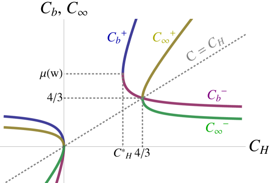
Figure 1: The values of the roots $C_{b}^{\pm}$ and $C_{\infty}^{\pm}$ are plotted as functions of $C_{H}$. The plot corresponds to the value $w=0$ but the relative position of these four quantities remain unchanged for other values of $w$ in the range $0\leq w\leq 1$.

Before closing this subsection, it is instructive to rewrite the basic equations in terms of $C_{b}^{\pm}$ and $C_{\infty}^{\pm}$, assuming their existence. The equations of motion read

$$\frac{{\rm d}C}{{\rm d}\tau} =f_{C}(h,C)=-\frac{3(1+w)}{2}\frac{h}{C-C_{H}}(C-C_{\infty}^{+})(C-C_{\infty}^{-})\,,$$ (42)

$$\frac{{\rm d}h}{{\rm d}\tau} =f_{h}(h,C)=-h^{2}-\frac{1+3w}{2}\frac{C}{C-C_{H}}(C-C_{b}^{+})(C-C_{b}^{-})\,,$$ (43)

while the two constraints are now given by

$${\cal R}_{m} =\frac{9}{3-2C_{H}}(C-C_{\infty}^{+})(C-C_{\infty}^{-})\geq 0\qquad(M)\,,$$ (44)

$$\frac{1}{a}\frac{{\rm d}^{2}a}{{\rm d}\tau^{2}} =-\frac{1+3w}{2}\frac{C}{C-C_{H}}(C-C_{b}^{+})(C-C_{b}^{-})\geq 0\qquad(A)\,.$$ (45)

Before investigating the stability of the fixed points in the next subsection, let us mention another special value of $C$, namely $C_{H}$, where the equations of motion become singular. The limit $C\rightarrow C_{H}$ corresponds to a curvature singularity, since $\dot{H}$ diverges in this limit. We encountered the same curvature singularity in our study of flat FLRW solutions in massive gravity on de Sitter Langlois:2012hk .

III.2 Stability of the fixed points

In order to understand qualitatively the evolution in the phase space, it is useful to study the evolution of linear perturbations around the fixed points that we have identified. Introducing the perturbations

$$\delta C\equiv C-C_{\mathrm{fixed}}\,,\qquad\delta h\equiv h-h_{\mathrm{fixed}}\,,$$ (46)

and linearizing the evolution equations with respect to $\delta C$ and $\delta h$, we obtain a linear system of the form

$$\frac{{\rm d}}{{\rm d}\tau}\begin{pmatrix}\delta C\\ \delta h\end{pmatrix}=\begin{pmatrix}\displaystyle\frac{{\partial}f_{C}}{{\partial}C}&\displaystyle\frac{{\partial}f_{C}}{{\partial}h}\\ \displaystyle\frac{{\partial}f_{h}}{{\partial}C}&\displaystyle\frac{{\partial}f_{h}}{{\partial}h}\end{pmatrix}_{\mathrm{fixed}}\begin{pmatrix}\delta C\\ \delta h\end{pmatrix}\quad\equiv\quad\mathbf{E}\ \begin{pmatrix}\delta C\\ \delta h\end{pmatrix}\,,$$ (47)

where $\mathbf{E}$ is a short notation for the $2\times 2$ matrix on the right hand side. The stability properties of the system around any fixed point can be deduced from the eigenvalues of its evolution matrix ${\mathbf{E}}$,

$${\cal E}_{1,2}=\frac{1}{2}\left({\mathrm{T}r}({\mathbf{E}})\pm\sqrt{{\mathrm{T}r}({\mathbf{E}})^{2}-4{\mathrm{D}et}({\mathbf{E}})}\right)\,.$$ (48)

If ${\mathrm{D}et}({\mathbf{E}})<0$, the eigenvalues are real and have different sign: the fixed point is a saddle point. If ${\mathrm{D}et}({\mathbf{E}})>0$, the two eigenvalues, when real, have the same sign, which is given by ${\mathrm{T}r}({\mathbf{E}})$: if both eigenvalues are negative, the fixed point is an attractor because all flows converge towards it; conversely, if both eigenvalues are positive, the fixed point is a repeller. Moreover, depending whether the eigenvalues are real or imaginary, the fixed point is said to be nodal or spiral, respectively.

Let us first consider the fixed points defined by $C=C_{b}^{\pm}$, which are located on the axis $h=0$. Their evolution matrix reads

$${\mathbf{E}}=\begin{pmatrix}0&\displaystyle\frac{{\partial}f_{C}}{{\partial}h}\\ \displaystyle\frac{{\partial}f_{h}}{{\partial}C}&0\\ \end{pmatrix}_{(C_{b}^{\pm},0)}$$ (49)

with

$$\frac{{\partial}f_{C}}{{\partial}h} =-\frac{3(1+w)}{1+3w}\frac{C_{H}}{C_{b}^{\pm}-C_{H}}\left(C_{b}^{\pm}-\frac{4}{3}\right)\,,\qquad\frac{{\partial}f_{h}}{{\partial}C}=-\frac{(2+3w)C_{H}}{C_{b}^{\pm}-C_{H}}\left[C_{b}^{\pm}-\mu(w)\right]\,.$$ (50)

The trace and the determinant of the matrix are thus

$${\mathrm{T}r}({\mathbf{E}})=0\,,\qquad{\mathrm{D}et}({\mathbf{E}})=-\frac{{\partial}f_{C}}{{\partial}h}\frac{{\partial}f_{h}}{{\partial}C}=-\frac{3(1+w)(2+3w)}{1+3w}\frac{C_{H}^{2}}{(C_{b}^{\pm}-C_{H})^{2}}\left(C_{b}^{\pm}-\frac{4}{3}\right)\left(C_{b}^{\pm}-\mu(w)\right)\,.$$ (51)

The eigenvalues are real if ${\mathrm{D}et}({\mathbf{E}})<0$, giving a saddle point; purely imaginary if ${\mathrm{D}et}({\mathbf{E}})>0$, in which case the fixed point is spiral. According to Fig.1, one can easily see that the case ${\mathrm{D}et}({\mathbf{E}})>0$ is possible only for the fixed point $C_{b}^{-}$, provided $C_{H}$ is the range $C_{H}^{*}(w)<C_{H}<4/3$. In all other cases, the fixed points $C_{b}^{\pm}$ are saddle points.

One can proceed in a similar manner for the fixed points $C_{\infty}^{\pm}$. Their evolution matrix reduces to

$${\mathbf{E}}=\begin{pmatrix}\displaystyle\frac{{\partial}f_{C}}{{\partial}C}&0\\ \displaystyle\frac{{\partial}f_{h}}{{\partial}C}&\displaystyle\frac{{\partial}f_{h}}{{\partial}h}\\ \end{pmatrix}_{(C_{\infty},h_{\infty})}$$ (52)

with

$$\frac{{\partial}f_{C}}{{\partial}C} =-3(1+w)h_{\infty}\,,\qquad\frac{{\partial}f_{h}}{{\partial}C}=-(1+3w)C_{\infty}\,,\qquad\frac{{\partial}f_{h}}{{\partial}h}=-2h_{\infty}\,,$$ (53)

where $h_{\infty}=\pm C_{\infty}$. The two eigenvalues of the matrix are simply $-3(1+w)h_{\infty}$ and $-2h_{\infty}$. The fixed points in the region $H>0$ are thus attractors while the fixed points in the $H<0$ are repellers.

Let us mention briefly the fixed point at the origin, which is a saddle point. Since it is located at a corner of the physical phase space, only the quadrant on its right is relevant.

It is also worth noticing that the vector field tangent to the flow becomes vertical on the axes $C=C_{\infty}^{\pm}$, which means that trajectory cannot cross these axes. As a consequence, if the constraint (44) is satisfied initially, it will remain so in the future. However, this is not the case for the constraint (45). Indeed, one can check that the flow is not vertical on the axes $C=C_{b}^{\pm}$, so that a trajectory can a priori cross these boundaries in phase space. Therefore, even if the constraint $\ddot{a}>0$ is satisfied initially, some of the phase space trajectories can reach $\ddot{a}=0$ during their evolution. Although this transition is perfectly regular from the point of view of Friedmann’s equations, it is problematic from the point of view of the underlying massive gravity theory where $\ddot{a}=0$ corresponds to $\dot{f}=0$, in which case the tensor $f_{\mu\nu}$ becomes degenerate. In other words, the coordinate transformation between the abstract de Sitter space and the FLRW coordinates, embodied by the Stückelberg fields, becomes singular: $\det(\partial_{\mu}\phi^{A})=0$. It is intriguing that this determinant singularity, following the terminology used in Gratia:2013gka , which signifies a breakdown of the massive gravity framework, at least in its present formulation, does not appear at all in the cosmological evolution at the level of the Friedmann equations.

III.3 Global analysis

After having analysed the stability of the various fixed points separately, we now present a global discussion on the existence of the fixed points and their stability, depending on the value of the parameter $C_{H}$ (or equivalently $\lambda$). In each case, we will draw the corresponding phase portrait.

As discussed earlier, and illustrated in Fig. ​1, the existence of the various fixed points that we have identified depends on the value of $C_{H}$. The fixed points $C_{b}^{\pm}$ exist only if $C_{H}\leq 0$ or $C_{H}\geq C_{H}^{*}(w)$, whereas the existence of the fixed points $C_{\infty}^{\pm}$ requires $C_{H}\leq 0$ or $C_{H}>4/3$. Taking also into account the special value $C_{H}=3/2$ (corresponding to infinite $\lambda$) for which the constraint (M) is not defined, one can distinguish five intervals for the parameter $C_{H}$, separated by the values $3/2$, $4/3$, $C_{H}^{*}(w)$ and $0$, in decreasing order.

III.3.1 Case $C_{H}>3/2$ (or $\lambda<-1$)

This case is illustrated in Fig. 2. All fixed points $C_{b}^{\pm}$ and $C_{\infty}^{\pm}$ exist and they are ordered as

$$0<C_{\infty}^{-}\leq C_{b}^{-}\leq C_{H}\leq C_{\infty}^{+}<C_{b}^{+}\,.$$ (54)

The second constraint (M) implies that the trajectory must be inside the region

$$C_{\infty}^{-}\leq C\leq C_{\infty}^{+}\qquad(M)$$ (55)

which contains $C_{b}^{-}$ but not $C_{b}^{+}$. Within this region, the system accelerates, i.e. satisfies the constraint (A), only in the two subregions

$$C_{\infty}^{-}\leq C\leq C_{b}^{-}\quad{\mathrm{and}}\quad C_{H}\leq C\leq C_{\infty}^{+}\qquad(M)\,\&\,(A)\,.$$ (56)

In the first region, one finds three fixed points: the repeller $(C_{\infty}^{-},-C_{\infty}^{-})$, the attractor $(C_{\infty}^{-},+C_{\infty}^{-})$ and $(C_{b}^{-},0)$ on the axis. According to our discussion of the previous subsection, the eigenvalues for the fixed point $C_{b}^{-}$ are real (and opposite) because ${\mathrm{D}et}({\mathbf{E}})<0$. The cosmological flows in this region are depicted in Fig. 2. As one can see, there exist some solutions that reach the determinant singularity on the axis $C=C_{b}^{-}$.

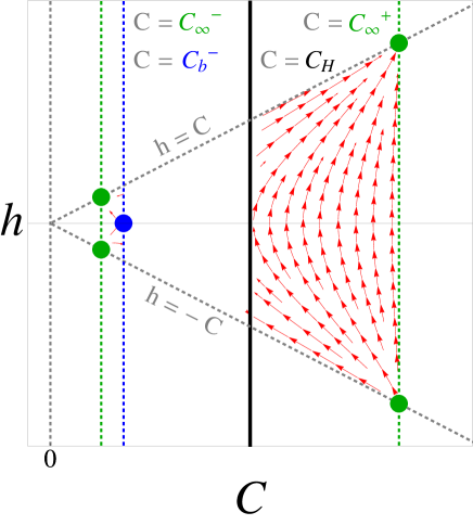
(a) Global picture

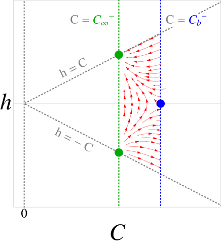
(b) Enlargement of the region $C_{\infty}^{-}\leq C\leq C_{b}^{-}$

Figure 2: Phase diagram in the case $C_{H}>3/2$ (i.e. $\lambda<-1$). All fixed points are defined, but the fixed point $(C_{b}^{+},0)$ is outside of the region allowed by the constraint (M), and is therefore not represented. The region between $C_{b}^{-}$ and $C_{H}$ is forbidden by the constraint (A). The trajectories that approach $C=C_{H}$ are singular in this limit, which means they cannot cross the boundary $C=C_{H}$.

In the region $C_{H}\leq C\leq C_{\infty}^{+}$, one finds trajectories that start in the asymptotic past at the fixed point $(C_{\infty}^{-},-C_{\infty}^{-})$, in a contracting phase, and evolve to reach in the asymptotic future the symmetric fixed point $(C_{\infty}^{-},C_{\infty}^{-})$. They represent perfect examples of bouncing cosmologies with a regular behaviour. Other trajectories end, or start, on the boundary $C=C_{H}$, which corresponds to a curvature singularity (where $\dot{H}$ diverges) and do not experience bouncing.

III.3.2 Case $4/3\leq C_{H}<3/2$ (or $\lambda\geq 8$)

In this parameter range, we still have the existence of all fixed points with the same ordering (54) as in the previous case. However, the constraint (M) now excludes the region between $C_{\infty}^{-}$ and $C_{\infty}^{+}$, so that the allowed region is

$$C\leq C_{\infty}^{-}\quad{\rm or}\quad C\geq C_{\infty}^{+}\qquad(M)\,.$$ (57)

The fixed point $C_{b}^{-}$ and the singular line $C=C_{H}$ are thus irrelevant in this case. Taking into account the constraint (A) as well, the second region gets restricted so that the final allowed regions are

$$C\leq C_{\infty}^{-}\quad{\mathrm{and}}\quad C_{\infty}^{+}\leq C\leq C_{b}^{+}\qquad(M)\,\&\,(A)\,.$$ (58)

In the region $C\leq C_{\infty}^{-}$, all trajectories are bouncing solutions, which start from the repeller $(C,h)=(C_{\infty}^{-},-C_{\infty}^{-})$ and end at the attractor $(C,h)=(C_{\infty}^{-},C_{\infty}^{-})$. In the second region, $C_{\infty}^{+}\leq C\leq C_{b}^{+}$, there exist bouncing trajectories between the fixed points $(C_{\infty}^{+},-C_{\infty}^{+})$ and $(C_{\infty}^{+},C_{\infty}^{+})$, but also trajectories that reach the boundary $C_{b}^{+}$. For the fixed point $C_{b}^{+}$, we find that the eigenvalues are real (and opposite) as in the previous case. The phase diagram is depicted in Fig. 3.

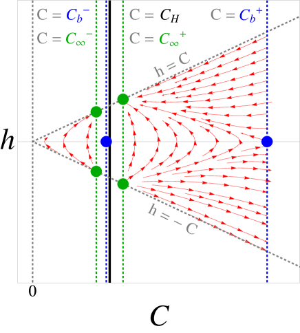
Figure 3: Phase diagram in the case $4/3<C_{H}<3/2$ (i.e. $\lambda>8$). All fixed points are defined. The region between $C_{\infty}^{-}$ and $C_{\infty}^{+}$, which contains the fixed point $(C_{b}^{-},0)$ and the axis $C=C_{H}$, is forbidden by the constraint (M). The region above $C_{b}^{+}$ is forbidden by the constraint (A). In the left region, all solutions are bouncing and relate $(C_{\infty}^{-},-C_{\infty}^{-})$ to $(C_{\infty}^{-},C_{\infty}^{-})$. In the right region, one finds bouncing solutions that evolve from $(C_{\infty}^{+},-C_{\infty}^{+})$ to $(C_{\infty}^{+},C_{\infty}^{+})$, but also solutions that evolve into or from the determinant singularity.

We should consider separately the degenerate case $C_{H}=4/3$, for which

$$C_{\infty}^{+}=C_{\infty}^{-}=C_{b}^{-}=C_{H}=\frac{4}{3}\,.$$ (59)

The two repellers ($h<0$) merge into a single repeller at $(4/3,-4/3)$. Similarly, the two attractors with $h>0$ merge into a single attractor at $(4/3,4/3)$. Moreover, the fixed point $C_{b}^{-}$ disappears since the right hand side of (43) reduces to

$$f_{h}(h,C)=-h^{2}-\frac{1+3w}{2}C(C-C_{b}^{+})\,.$$ (60)

The exclusion region due to the constraint (M) disappears and the allowed region satisfying the constraint (A) is simply

$$0<C\leq C_{b}^{+}\qquad(A)\,.$$ (61)

The qualitative behaviour is exactly the same as in the allowed region of the non degenerate case, as illustrated in Fig. 4.

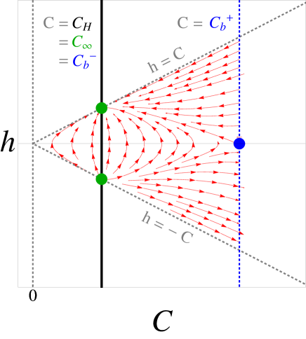
Figure 4: Phase diagram in the special case $C_{H}=4/3$ (i.e. $\lambda=8$). The fixed points $C_{\infty}^{-}$ and $C_{\infty}^{+}$ now coincide, so that the intermediate forbidden region of Fig. 3 has disappeared. Apart this difference, the behavior in the rest of the phase space is quite similar to that of Fig. 3.

III.3.3 $C_{H}^{*}(w)\leq C_{H}<4/3$ (i.e. $\lambda^{*}(w)\leq\lambda<8$)

In this case, the fixed points $C_{\infty}^{\pm}$ do not exist and we are left with the fixed points $C_{b}^{\pm}$ on the $H=0$ axis. The hierarchy is now given by

$$C_{H}<C_{b}^{-}\leq C_{b}^{+}\,.$$ (62)

Since $C_{H}<3/2$ and the two roots $C_{\infty}^{+}$ and $C_{\infty}^{-}$ are imaginary, the constraint (M) is automatically satisfied, whereas the constraint (A) implies

$$C\leq C_{H}\quad{\mathrm{or}}\quad C_{b}^{-}\leq C\leq C_{b}^{+}\qquad(A)\,.$$ (63)

We thus find an excluded region between $C_{H}$ and $C_{b}^{-}$.

The behavior of the perturbations around $C_{b}^{-}$ also differs from the previous cases since we now have $4/3<C_{b}^{-}<\mu(w)$, which implies ${\mathrm{D}et}({\mathbf{E}})>0$. The eigenvalues for $C_{b}^{-}$ are thus purely imaginary, which corresponds to a spiral point, as illustrated in Fig. 5. The other fixed point $C_{b}^{+}$ remains a saddle point.

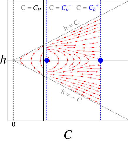
Figure 5: Phase diagram in the case $C_{H}^{*}(w)\leq C_{H}<4/3$ (i.e. $\lambda^{*}(w)\leq\lambda<8$). The fixed points $C_{\infty}^{\pm}$ do not exist. Two regions are forbidden by the constraint (A): the first one between $C_{H}$ and $C_{b}^{-}$, the second one beyond $C_{b}^{+}$. All solutions start and end on singular boundaries: curvature singularity in the left region and determinant singularity in the right region.

In the region $C\leq C_{H}$, there is no fixed point (except the origin) and the trajectories evolve from the line $C=C_{H}$ with $h<0$ towards the same line with $h>0$. All solutions correspond to bouncing solutions but they are singular in the past and in the future. In the second region, $C_{b}^{-}\leq C\leq C_{b}^{+}$, one also finds bouncing trajectories starting and ending on the line $C=C_{b}^{-}$. We also find solutions that are not bouncing: contracting solutions that go from the line $C=C_{b}^{-}$ to the line $C=C_{b}^{+}$ and expanding solutions that go from $C=C_{b}^{+}$ to the boundary $C=C_{b}^{-}$.

Finally, let us discuss the special case where the two fixed points $C_{b}^{-}$ and $C_{b}^{+}$ become degenerate, which occurs for the value $C_{H}=C_{H}^{*}(w)$, in which case

$$C_{b}^{\pm}=\mu(w)\,.$$ (64)

The constraint (A) then imposes

$$C<C_{H}\,,$$ (65)

which means that the only fixed point $C_{b}^{-}\equiv C_{b}^{+}$ is outside the allowed region. As illustrated in Fig. 6, the situation is quite analogous to what happens in the left region ($C<C_{H}$) of the non degenerate case.

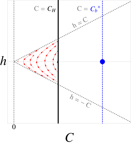
Figure 6: Phase diagram in the special case $C_{H}=C_{H}^{*}(w)$ (i.e. $\lambda=\lambda^{*}(w)$). The fixed points $C_{b}^{-}$ and $C_{b}^{+}$ now coincide, but are in the region forbidden by (A). All solutions in the allowed region are bouncing, evolving from the negative part to the positive part of the $C=C_{H}$ axis, characterized by a curvature singularity.

III.3.4 $0<C_{H}<C_{H}^{*}(w)$ (i.e. $0<\lambda<\lambda^{*}(w)$)

There is no fixed point in this case and the constraint (A) imposes the condition

$$C\leq C_{H}\,.$$ (66)

The evolution is phase space is similar to the special limit $C_{H}=C_{H}^{*}(w)$ discussed previously. Once again, all solutions are bouncing and connect the lower $C=C_{H}$ axis to its upper part.

III.3.5 $C_{H}<0$ (i.e. $-1<\lambda<0$)

In this parameter range, only the fixed points $C_{\infty}^{+}$ and $C_{b}^{+}$ are defined, since the solutions $C_{\infty}^{-}$ and $C_{b}^{-}$ are negative. Consequently, the constraint (M) imposes the restriction

$$C\geq C_{\infty}^{+}\qquad(M)$$ (67)

while the constraint (A) requires

$$C<C_{b}^{+}\qquad(A)\,.$$ (68)

The allowed region is therefore between $C_{\infty}^{+}$ and $C_{b}^{+}$. As illustrated in Fig. 7, one finds bouncing solutions evolving from the fixed point $(C_{\infty}^{+},-C_{\infty}^{+})$ towards $(C_{\infty}^{+},C_{\infty}^{+})$. The other solutions start or end at the boundary $C=C_{b}^{+}$ corresponding to the determinant singularity.

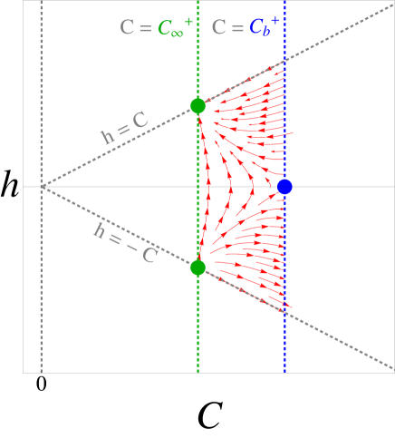
Figure 7: Phase diagram in the case $C_{H}<0$ (i.e. $-1<\lambda<0$). There are three fixed points and the phase portrait is quite similar to that of the right region in Fig.3.

IV Summary and discussion

In this paper, we have studied closed FLRW solutions in the context of massive gravity with de Sitter as fiducial metric. We have found that bouncing solutions are generic when cosmological matter satisfies the strong energy condition ($w>-1/3$). This is in contrast with classical general relativity where closed bouncing solutions require cosmological matter that violates the strong energy condition. The different outcome in the massive gravity framework is due to the presence of extra terms, which arise from the potential term in the gravitational action.

We have also investigated the dynamical evolution of the cosmological system by resorting to standard phase space analysis. Introducing a two-dimensional phase space spanned by the variables $C$ and $h=H/H_{c}$, we have identified the fixed points of the system. Their number depends on $\lambda=m_{g}^{2}/H_{c}^{2}$, i.e. the square of the ratio between the graviton mass and the fiducial Hubble parameter. The maximal number of fixed points (ignoring the origin) is six: two on the axis $h=0$ ($C_{b}^{-}$ and $C_{b}^{+}$), and two pairs of points symmetric with respect to the $h=0$ axis and localized on the $h=\pm C$ lines. There also exists a vertical line $C=C_{H}$ where the solutions encounter a curvature singularity. For all values of the parameter $\lambda$, we have found that bouncing solutions are generic.

In summary, the cosmological solutions can have three different fates (and corresponding origins, by time reversal). These fates are analogous to those encountered in the spatially flat case, discussed in our previous work Langlois:2012hk . The first fate is a regular asymptotic de Sitter regime (corresponding to $C_{\infty}$). The second possibility is that the Universe ends in a curvature singularity ($C=C_{H}$). Finally, the third possibility is to reach a singularity specific to massive gravity, on the boundary $C=C_{b}$, where $\dot{f}=0$ and the tensor $f_{\mu\nu}=0$ thus becomes degenerate. Intriguingly, there is no trace of this singular behaviour at the level of the effective Friedmann equations. This means that if one works directly with the generalized Friedmann equations, without worrying about the underlying theory, one can simply continue the cosmological evolution across this boundary where nothing seems to happen, except that the solution is decelerating after the transition. This might indicate that this type of singularity could be resolved in an extended framework of massive gravity, as suggested recently in Gratia:2013gka .

References

References

- (1) C. de Rham, G. Gabadadze and A. J. Tolley, Phys. Rev. Lett. 106, 231101 (2011) [arXiv:1011.1232 [hep-th]].
- (2) D. G. Boulware and S. Deser, Phys. Rev. D 6, 3368 (1972).
- (3) G. D’Amico, C. de Rham, S. Dubovsky, G. Gabadadze, D. Pirtskhalava and A. J. Tolley, Phys. Rev. D 84, 124046 (2011) [arXiv:1108.5231 [hep-th]].
- (4) A. E. Gumrukcuoglu, C. Lin and S. Mukohyama, JCAP 1111, 030 (2011) [arXiv:1109.3845 [hep-th]].
- (5) S. F. Hassan and R. A. Rosen, JHEP 1107, 009 (2011) [arXiv:1103.6055 [hep-th]]; S. F. Hassan, R. A. Rosen and A. Schmidt-May, JHEP 1202, 026 (2012) [arXiv:1109.3230 [hep-th]];
- (6) M. Fasiello and A. J. Tolley, JCAP 1211 (2012) 035 [arXiv:1206.3852 [hep-th]].
- (7) D. Langlois and A. Naruko, Class. Quant. Grav. 29, 202001 (2012) [arXiv:1206.6810 [hep-th]].
- (8) K. Koyama, G. Niz and G. Tasinato, Phys. Rev. Lett. 107, 131101 (2011) [arXiv:1103.4708 [hep-th]]. K. Koyama, G. Niz and G. Tasinato, Phys. Rev. D 84, 064033 (2011) [arXiv:1104.2143 [hep-th]]. A. H. Chamseddine and M. S. Volkov, Phys. Lett. B 704, 652 (2011) [arXiv:1107.5504 [hep-th]]. P. Gratia, W. Hu and M. Wyman, Phys. Rev. D 86 (2012) 061504 [arXiv:1205.4241 [hep-th]]. T. Kobayashi, M. Siino, M. Yamaguchi and D. Yoshida, Phys. Rev. D 86, 061505 (2012) [arXiv:1205.4938 [hep-th]]. M. S. Volkov, Phys. Rev. D 86 (2012) 061502 [arXiv:1205.5713 [hep-th]]. V. Baccetti, P. Martin-Moruno and M. Visser, Class. Quant. Grav. 30, 015004 (2013) [arXiv:1205.2158 [gr-qc]]. A. E. Gumrukcuoglu, C. Lin and S. Mukohyama, Phys. Lett. B 717, 295 (2012) [arXiv:1206.2723 [hep-th]].
- (9) G. D’Amico, G. Gabadadze, L. Hui and D. Pirtskhalava, arXiv:1206.4253 [hep-th].
- (10) Q. -G. Huang, Y. -S. Piao and S. -Y. Zhou, Phys. Rev. D 86, 124014 (2012) [arXiv:1206.5678 [hep-th]].
- (11) A. De Felice, A. E. Gumrukcuoglu, C. Lin and S. Mukohyama, arXiv:1304.0484 [hep-th].
- (12) G. Tasinato, K. Koyama and G. Niz, arXiv:1304.0601 [hep-th].
- (13) F. T. Falciano, M. Lilley and P. Peter, Phys. Rev. D 77, 083513 (2008) [arXiv:0802.1196 [gr-qc]].
- (14) L. Alberte, Int. J. Mod. Phys. D 21, 1250058 (2012) [arXiv:1110.3818 [hep-th]].
- (15) C. de Rham and S. Renaux-Petel, JCAP 1301 (2013) 035 [arXiv:1206.3482 [hep-th]].
- (16) P. Gratia, W. Hu and M. Wyman, arXiv:1305.2916 [hep-th].