On the simultaneous evolution
of massive protostars and their host cores

Abstract

Studies of the evolution of massive protostars and the evolution of their host molecular cloud cores are commonly treated as separate problems. However, interdependencies between the two can be significant. Here, we study the simultaneous evolution of massive protostars and their host molecular cores using a multi-dimensional radiation hydrodynamics code that incorporates the effects of the thermal pressure and radiative acceleration feedback of the centrally forming protostar. The evolution of the massive protostar is computed simultaneously using the stellar evolution code STELLAR, modified to include the effects of variable accretion. The interdependencies are studied in three different collapse scenarios. For comparison, stellar evolutionary tracks at constant accretion rates and the evolution of the host cores using pre-computed stellar evolutionary tracks are computed.

The resulting interdependencies of the protostellar evolution and the evolution of the environment are extremely diverse and depend on the order of events, in particular the time of circumstellar accretion disk formation with respect to the onset of the bloating phase of the star. Feedback mechanisms affect the instantaneous accretion rate and the protostar’s radius, temperature and luminosity on timescales $t\leq 5\mbox{ kyr}$, corresponding to the accretion timescale and Kelvin-Helmholtz contraction timescale, respectively. Nevertheless, it is possible to approximate the overall protostellar evolution in many cases by pre-computed stellar evolutionary tracks assuming appropriate constant average accretion rates.

1 Introduction

Massive luminous protostars strongly influence their environment by e.g. thermal feedback, radiative acceleration feedback, protostellar winds, and ionization. These various feedback mechanisms are of great interest in the context of clustered star formation and are investigated in numerical simulations (e.g. Yorke & Sonnhalter 2002; Krumholz et al. 2007, 2009; Peters et al. 2010a; Kuiper et al. 2010a; Peters et al. 2011; Kuiper et al. 2011; Cunningham et al. 2011; Dale & Bonnell 2011; Kuiper et al. 2012) and observations (e.g. Beuther et al. 2002a; Kraus et al. 2010; Wang et al. 2011; Wheelwright et al. 2012). Later in their evolution after dissipation of their accretion disks, massive stars will continue to influence their surroundings via e.g. ionization, stellar winds and supernova explosions. The interested reader is refered to Mac  Low & Klessen (2004), Beuther et al. (2007), Zinnecker & Yorke (2007), and McKee & Ostriker (2007) for recent reviews on the field of (massive) star formation.

The physical state of a molecular core affects the accretion rate onto the embedded protostellar objects. The accretion rate onto the protostar itself is significantly affected by the formation of a circumstellar disk, by details of the angular momentum transport within the disk and by the launching of magnetic or radiation driven outflows, all of which in turn affect the surrounding molecular core. Jets and outflows are ubiquitously observed in high-mass star forming regions (e.g. Shepherd & Churchwell 1996; Zhang et al. 2001; Beuther et al. 2002b; Beltran et al. 2006; Zhang et al. 2007; Fallscheer et al. 2009; Leurini et al. 2011). Although direct observations of accretion disks in high-mass star forming regions are hampered by the fact that they are presumably short-lived, deeply embedded and at large distances, their existence can indirectly be inferred from the collimation of the jets and outflows (Gómez et al. 2003; Brooks et al. 2007; Furuya et al. 2008; Guzmán et al. 2012). Furthermore, the number of known disk candidates is rising (Nielbock et al. 2007; Bik et al. 2008; Beuther & Walsh 2008; Beuther et al. 2009) and at least disk-like structures are detected around massive protostellar objects (Bik & Thi 2004; Cesaroni et al. 2005; Beuther et al. 2005; Patel et al. 2005; Chini et al. 2006; Kraus et al. 2010; Beuther et al. 2010; Quanz et al. 2010; Preibisch et al. 2011). The potentially best studied disk candidates are AFGL 490 (Harvey et al. 1979; Torrelles et al. 1986; Chini et al. 1991; Davis et al. 1998; Lyder et al. 1998; Schreyer et al. 2002, 2006) and IRAS 20126+4104 (Wilking et al. 1989; Cesaroni et al. 1997; Zhang et al. 1998; Cesaroni et al. 1999; Hofner et al. 1999; Cesaroni et al. 2005; Sridharan et al. 2005). For the latest reviews on observational evidence for accretion disks around massive protostars, please see Zhang (2005) and Cesaroni et al. (2007).

Stahler et al. (1980) included the effect of accretion on the protostellar evolution for low-mass stars. For intermediate-mass protostars, Palla & Stahler (1991, 1992) studied the evolution of protostars including the effect of different intermediate accretion rates. Behrend & Maeder (2001) compute the protostellar evolution of massive stars assuming growing (non-constant) accretion rates. McKee & Tan (2003) present a simplified calculation of the evolution of the radius of a protostar and determine the protostellar accretion luminosity in a one-zone protostellar evolution model. In Yorke & Bodenheimer (2008, ASP Conf.Ser. 387, 189), Hosokawa & Omukai (2009) and Hosokawa et al. (2010) stellar evolutionary tracks for massive protostars are computed under the assumption of a time-independent constant accretion rate. Using the pre-computed stellar evolutionary tracks by Hosokawa & Omukai (2009) as a subgrid model for the forming massive protostar, Kuiper et al. (2010a) and Kuiper et al. (2011) determined the evolution of their corresponding massive pre-stellar cores. Here we present and discuss the first simulations that take into account self-consistently the mutual feedback effects of an evolving massive protostar within the simultaneously evolving natal core.

2 Methods

We have incorporated the stellar evolution code STELLAR (Bodenheimer et al. 2007) modified by incorporating variable accretion (Yorke & Bodenheimer 2008) into our radiation-hydrodynamical framework for the evolution of the collapsing pre-stellar core (introduced in Kuiper et al. 2010b, a, 2011).

2.1 Solving for the evolution of the pre-stellar core

To follow the evolution of the gas and dust of the collapsing pre-stellar core, we solve the equations of compressible radiation-hydrodynamics, including self-gravity and shear-viscosity, as described in Kuiper et al. (2010a). For the basic hydrodynamics solver, we use the open source MHD code Pluto, described in Mignone et al. (2007). As a special feature, our radiation transport solver takes into account the radiation pressure feedback by the forming protostar via a hybrid radiation transport approach, i.e. using a frequency-dependent ray-tracing step for the stellar irradiation and a gray flux-limited diffusion approximation for the thermal dust emission. Recently, in Kuiper et al. (2012), we depicted the importance of the direct stellar irradiation feedback during the formation of massive stars regarding the stability of radiation-pressure-dominated cavities forming in the bipolar direction. The derivation, the numerics, and tests of this hybrid scheme are given in Kuiper et al. (2010b). In Kuiper & Klessen (2013), the reliability of this hybrid approach, the gray approximation, and the flux-limited diffusion approximation is compared to Monte-Carlo radiation transport results for circumstellar disks of a wide range of optical depths.

Here, we restrict ourselves to studies of the evolution of pre-stellar cores in axial symmetry only, which allows us to vary important parameters over a wide range. As we shall show, the main impact on the protostellar accretion rate will be given by the formation of an accretion disk and the launching of bipolar outflows. Hence, the restriction to axial symmetry does not denote any limitation to the feedback mechanisms onto the actual protostellar evolution. In contrast to our previous studies, the evolution of the protostar and the evolution of the pre-stellar core are computed simultaneously.

2.2 Solving for the evolution of the protostar

The textbook Bodenheimer et al. (2007) includes a CD-ROM with the program package STELLAR, which implicitly solves the equations of stellar structure in spherical symmetry via the Henyey method, assuming a gray atmosphere. Convection is treated in the context of mixing-length theory. A nuclear burning reaction network for pp- and CNO-hydrogen burning and helium burning up to the 3-$\alpha$ process is included. The atmosphere module of STELLAR has been modified to allow “cold” accretion of material (Yorke & Bodenheimer 2008) onto the atmosphere, i.e. it is assumed that most of the heat produced in an accretion shock is radiated away, before it settles onto the star. The accretion luminosity $L_{\mathrm{a}cc}$ is accounted for separately, i.e. $L_{\mathrm{t}ot}=L_{*}+L_{\mathrm{a}cc}$, whereby

$$L_{\mathrm{acc}}=\eta\frac{G~{}M_{*}}{R_{*}}~{}\dot{M}_{*}\;,$$ (1)

where $L_{*}$, $M_{*}$, $R_{*}$, and $\dot{M}_{*}$ are the (proto)stellar luminosity, mass and radius and the mass accretion rate onto the (proto)star, respectively. $\eta$ is a dimensionless parameter of order unity but less than one, which takes into account the fact that not all of the accretion’s kinetic energy is converted into radiative energy. For simplicity we use $\eta=1$.

As a starting model, we use a $0.05\mbox{ M}_{\odot}$ object in hydrostatic equilibrium with a radius of $0.56\mbox{ R}_{\odot}$ and a luminosity of $2.2\times 10^{-2}\mbox{ L}_{\odot}$.

3 Simulations overview, initial conditions, and numerical configuration

Tag	Stellar	Core	$\beta$	$E_{\mathrm{rot}}/E_{\mathrm{grav}}$	$\dot{M}_{*}$	$R_{*}^{\mathrm{max}}$	$M_{*}^{\mathrm{Disk}}$	$M_{*}^{\mathrm{Bloating}}$	$M_{*}^{\mathrm{ZAMS}}$
	evolution	evolution	$\rho\propto r^{\beta}$	[%]	$\mbox{ [}10^{-4}\mbox{ M}_{\odot}\mbox{ yr}^{-1}\mbox{]}$	$\mbox{ [R}_{\odot}\mbox{]}$	$\mbox{ [M}_{\odot}\mbox{]}$	$\mbox{ [M}_{\odot}\mbox{]}$	$\mbox{ [M}_{\odot}\mbox{]}$
RHD+SE A	Yes	Yes	$-2.0$	1.0	-	885	22	5.0 - 22.0	40
RHD+SE B	Yes	Yes	$-1.5$	1.7	-	456	7	3.9 - 12.0	30
RHD+SE C	Yes	Yes	$-1.5$	5.0	-	389	2.4	3.5 - 10.7	21
RHD A	No	Yes	$-2.0$	1.0	-	-	25	-	-
RHD B	No	Yes	$-1.5$	1.7	-	-	7	-	-
RHD C	No	Yes	$-1.5$	5.0	-	-	3.7	-	-
SE	Yes	No	-	-	30	1366	-	5.3 - 39.2	70
SE A	Yes	No	-	-	20	845	-	4.6 - 23.0	52
SE	Yes	No	-	-	10	498	-	3.7 - 13.0	32
SE B	Yes	No	-	-	9	462	-	3.6 - 12.2	30
SE C	Yes	No	-	-	7	377	-	3.5 -   9.9	25
SE	Yes	No	-	-	5	286	-	3.3 -   7.7	21
SE	Yes	No	-	-	1	31	-	2.6 -   3.9	10

Table 1: Overview of simulations performed. From left to right the columns denote the run tag, the code configuration, and whether or not the protostellar evolution and the evolution of the pre-stellar core are computed. For cases when the evolution of the molecular core is computed, the next two columns denote the initial density slope $\beta$ of the pre-stellar core and the initial ratio of rotational to gravitational energy $E_{\mathrm{rot}}/E_{\mathrm{grav}}$ of the pre-stellar core. The assumed constant accretion rate $\dot{M}_{*}$ given in the next column is only relevant when the evolution of the molecular core is not computed. The last four columns denote the resulting maximum protostellar radius $R_{*}^{\mathrm{max}}$, the resulting stellar mass $M_{*}^{\mathrm{Disk}}$, at which the (Keplerian) circumstellar disk is formed, the resulting stellar mass range $M_{*}^{\mathrm{Bloating}}$, in which the protostar bloats up to its maximum radius, and the resulting stellar mass $M_{*}^{\mathrm{ZAMS}}$, at which the protostar reaches the zero-age-main-sequence. Dashes are given when these parameters are not relevant for a particular sequence.

We performed three different types of numerical simulation: The main study consists of simulations taking into account the simultaneous evolution of the protostar within its collapsing pre-stellar host molecular core. These runs are labeled with “RHD+SE” (Radiation-Hydrodynamics + Stellar Evolution). We consider three different initial conditions of the pre-stellar core morphology, labeled “A”, “B”, and “C”, for which we vary the initial density slope and the ratio of rotational to gravitational energy. For comparison purposes we perform a second type of simulation, calculating the evolution of pre-stellar cores – with the three different initial conditions – using the pre-computed stellar evolutionary tracks by Hosokawa & Omukai (2009). These evolutionary tracks of massive stars depend on the stellar mass as well as on the actual accretion rate. We use polynomial fits to the mass relation up to tenth order for separated mass ranges and linear regression for the dependence on the instantaneous accretion rate, see Kuiper et al. (2010a) for details. The numerical framework of these runs is consistent with our previous simulations (Kuiper et al. 2010a, 2011, 2012) and the runs are labeled with “RHD”. The third type of simulation, also for the purpose of comparison, is computing stellar evolutionary tracks at given constant accretion rates, labeled “SE”.

The initial condition of the protostellar evolution is given by a $0.05\mbox{ M}_{\odot}$ object in hydrostatic equilibrium with a radius of $0.56\mbox{ R}_{\odot}$ and a luminosity of $2.2\times 10^{-2}\mbox{ L}_{\odot}$. The initial condition of the pre-stellar cores is given by an outer core radius of $0.1~{}\mbox{pc}$, a core mass of $100\mbox{ M}_{\odot}$, and a core temperature of $20~{}\mbox{K}$. The core is initially in rigid solid body rotation. Our computational grid employs spherical coordinates $(r,\theta)$ assuming axial symmetry with a non-constant radial distribution of grid points and a central sink cell of $10~{}\mbox{AU}$. The resolution of the grid at the inner computational boundary is about $1~{}\mbox{AU}$ in the radial as well as in the polar direction. The polar extent of the grid covers the angles from $0\arcdeg$ to $90\arcdeg$, assuming equatorial symmetry. Towards the outer computational boundary, the grid cell size increases linearly with radius. For more details on the numerical grid in use, the numerical solvers, and the sub-grid models such as shear viscosity and the dust model, please see Kuiper et al. (2010b) and Kuiper et al. (2010a).

An overview of all simulations performed is given in Table 1.

The outstanding event during the protostellar evolution – for non-negligible accretion – is its bloating phase. The increase and decrease of the stellar radius before and after the bloating phase, respectively, have a strong impact on the protostellar environment. The (first) outstanding event during the pre-stellar core collapse is the formation of a circumstellar accretion disk. To investigate the possible interdependencies of the protostellar and the host core evolution, we computed three different collapse scenarios, in which the circumstellar disk forms either at the end (run “A”), during (run “B”), or before (run “C”) the protostellar bloating phase.

4 Results

In this section we discuss the main outcome of the protostellar and the pre-stellar core evolution in the three different collapse scenarios in light of four main evolutionary phases: (I) pre-bloating, (II) bloating, (III) Kelvin-Helmholtz contraction, and (IV) main sequence, which we shall discuss in more detail below. Note that Hosokawa & Omukai (2009) and Hosokawa et al. (2010) use the terms “convection” and “swelling” for phases (I) and (II). The four phases of evolution presented here are consistent with the “cold disk accretion” evolution by Hosokawa et al. (2010), but in contrast to their assumed constant accretion rates, we use the accretion rate computed self-consistently from the evolution of the collapsing pre-stellar core, including the radiation pressure feedback of the forming star.

The protostellar evolution in the framework of the three scenarios is shown in the corresponding Hertzsprung-Russell diagrams and the evolution of the stellar radius with mass in Figs. 1 to 6. During phase (I) before the onset of bloating, the accretion timescale is much shorter (up to four orders of magnitude) than the Kelvin-Helmholtz contraction timescale of the newborn protostar. Energy transport within the protostar is initially primarily via convection, but the protostar later becomes radiative. In either case the protostar is not in thermal equilibrium and it eventually begins to expand rapidly when the Kelvin-Helmholtz timescale is longer than the accretion timescale. The maximum stellar radius and the mass range of the bloating phase (II) are given in Table 1. When the Kelvin-Helmholtz timescale becomes shorter than the accretion timescale (phase III), the protostar begins to contract toward the main sequence. This contraction is stopped when hydrogen burning begins (phase IV).

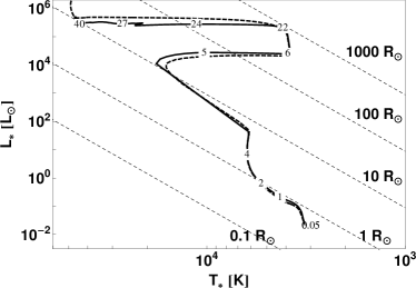
Figure 1: Hertzsprung-Russell diagram for the protostellar evolution in the collapse scenario “RHD+SE A” (solid line). The dashed stellar evolutionary track denotes the evolution of the protostar in a comparison run assuming a constant accretion rate of $2\times 10^{-3}\mbox{ M}_{\odot}\mbox{ yr}^{-1}$. The diagonal dashed lines denote lines of constant stellar radii as labeled. The small numbers along the stellar evolutionary track mark the protostellar mass.

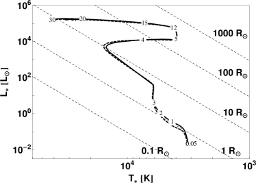
Figure 2: Hertzsprung-Russell diagram for the protostellar evolution in the collapse scenario “RHD+SE B”. The dashed stellar evolutionary track denotes the evolution of the protostar in a comparison run assuming a constant accretion rate of $9\times 10^{-4}\mbox{ M}_{\odot}\mbox{ yr}^{-1}$. Otherwise, symbols and numbers are as in Fig. 1.

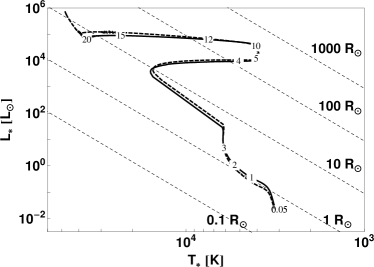
Figure 3: Hertzsprung-Russell diagram for the protostellar evolution in the collapse scenario “RHD+SE C”. The dashed stellar evolutionary track denotes the evolution of the protostar in a comparison run assuming a constant accretion rate of $7\times 10^{-4}\mbox{ M}_{\odot}\mbox{ yr}^{-1}$. Otherwise, symbols and numbers are as in Fig. 1.

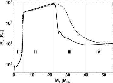
Figure 4: Evolution of the protostellar radius as a function of the protostellar mass in the collapse scenario “RHD+SE A” (solid line). The circle (at 22$\mbox{ M}_{\odot}$) denotes the onset of the formation of the circumstellar disk in the computational domain. The four phases: (I) pre-bloating, (II) bloating, (III) Kelvin-Helmholtz contraction, and (IV) main sequence evolution are as indicated. The dashed line denotes the evolution of the comparison run “SE A” assuming a constant accretion rate of $2\times 10^{-3}\mbox{ M}_{\odot}\mbox{ yr}^{-1}$.

Figure 5: Evolution of the protostellar radius as a function of the protostellar mass in the collapse scenario “RHD+SE B”; the four phases of evolution are as indicated. The circle (at 7$\mbox{ M}_{\odot}$) denotes the onset of the formation of the circumstellar disk in the computational domain. The dashed line denotes the evolution of the comparison run “SE B” assuming a constant accretion rate of $9\times 10^{-4}\mbox{ M}_{\odot}\mbox{ yr}^{-1}$.

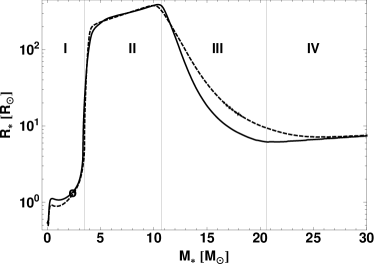
Figure 6: Evolution of the protostellar radius as a function of the protostellar mass in the collapse scenario “RHD+SE C”; the four phases of evolution are as indicated. The circle (at 2.4$\mbox{ M}_{\odot}$) denotes the onset of the formation of the circumstellar disk in the computational domain. The dashed line denotes the evolution of the comparison run “SE C” assuming a constant accretion rate of $7\times 10^{-4}\mbox{ M}_{\odot}\mbox{ yr}^{-1}$.

The effects of protostellar feedback on the pre-stellar core evolution in the three scenarios is most clearly shown by the evolution of the accretion rate onto the protostar in Figs. 7 to 9. In general, the interdependence of protostellar and the pre-stellar core evolution results in bursts of accretion and/or a non-constant, time-varying accretion rate. The formation of a circumstellar disk is accompanied by a sudden drop in the accretion rate followed by a short phase of enhanced accretion, although this effect is barely noticeable for case “RHD+SE B” (see Fig. 8), as the disk forms during phase (II).

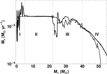
Figure 7: Evolution of the accretion rate as a function of the protostellar mass in the collapse scenario “RHD+SE A” (solid line); the four phases of evolution are as indicated. The dashed line denotes the evolution of the accretion rate in a comparison run (“RHD A”) using an a priori computed stellar evolutionary track. The circle (at 22$\mbox{ M}_{\odot}$) denotes the onset of the formation of the circumstellar disk in the computational domain.

Figure 8: Evolution of the accretion rate as a function of the protostellar mass in the collapse scenario “RHD+SE B”; the four phases of evolution are as indicated. The dashed line denotes the evolution of the accretion rate in a comparison run (“RHD B”) using an a priori computed stellar evolutionary track. The circle (at 7$\mbox{ M}_{\odot}$) denotes the onset of the formation of the circumstellar disk in the computational domain.

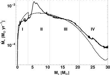
Figure 9: Evolution of the accretion rate as a function of the protostellar mass in the collapse scenario “RHD+SE C”; the four phases of evolution are as indicated. The dashed line denotes the evolution of the accretion rate in a comparison run (“RHD C”) using an a priori computed stellar evolutionary track. The circle (at 2.4$\mbox{ M}_{\odot}$) denotes the onset of the formation of the circumstellar disk in the computational domain.

5 Discussion

The results presented in the previous section demonstrate the interdependency of protostellar evolution and the evolution of its host molecular core. The three collapse scenarios considered differ in their density slopes and rotational to gravitational energy ratios, see Table 1. The differing initial angular momentum distributions result in circumstellar disk formation at different phases of the protostellar evolution. In run “A” the circumstellar disk forms at the end of protostellar bloating and the start of phase (III). In run “B” the circumstellar disk forms during the protostellar bloating phase (II). In run “C” the circumstellar disk forms prior to the protostellar bloating during phase (I).

5.1 Phase I: Before the bloating

One characteristic of the first phase is the domination of accretion luminosity over the intrinsic stellar luminosity, even for the collapse scenario “C” with the lowest initial accretion rate, see Fig. 10.

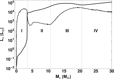
Figure 10: Accretion luminosity (dashed line) and protostellar luminosity (solid line) as a function of the protostellar mass in the collapse scenario “RHD+SE C”.

This dominant role of the accretion luminosity extends throughout phase I, which ends when the protostellar radius dramatically increases, lowering the specific energy of the material $\eta GM_{*}/R_{*}$ being accreted. Prior to bloating the radiative feedback of the centrally forming protostar onto the accretion flow depends strongly on the protostellar radius $R_{*}$ and the accretion rate $\dot{M}_{*}$ itself, see eq. (1). This yields a negative feedback mechanism with a time delay and results in quasi-periodic oscillations of the accretion rate: An increase of accretion at the surface of the star leads to a higher accretion luminosity, which in turn heats the nearby (dusty) protostellar environment. Radiative acceleration on the infalling dusty gas slows the accretion flow, resulting in a decrease of the accretion rate. After a delay given by the length of time the material needs to flow from the dust sublimation radius onto the surface of the star, the accretion luminosity decreases. This in turn reduced the radiative acceleration and allows the accretion rate to increase again. Altogether, this negative feedback coupling leads to a variability of the accretion rate in all three collapse scenarios investigated. In run “RHS+SE C”, this general behavior is modified by the early formation of the circumstellar disk, which lowers the direct interdependence between accretion rate and accretion luminosity. The material to be accreted by the star now has to pass through the circumstellar disk. Variations in the rate that the disk accretes material does not necessarily translate into analogous variations of the rate that the disk transports material to the stellar surface. The result is lower variability of accretion luminosity and accretion rate and a smoother transition into the bloating phase.

5.2 Phase II: Protostellar bloating phase

In all cases considered, accreting protostars pass through the “bloating phase” (II). The maximum stellar radius of the protostar strongly depends on the accretion history of the protostar; it ranges from $389\mbox{ R}_{\odot}$ (run “RHD+SE C”) up to $885\mbox{ R}_{\odot}$ (run “RHD+SE A”). Similar values are obtained at constant average accretion rates of $7\times 10^{-4}\mbox{ M}_{\odot}\mbox{ yr}^{-1}$ (run “SE C”) to $2\times 10^{-3}\mbox{ M}_{\odot}\mbox{ yr}^{-1}$ (run “SE A”), respectively.

During the bloating phase there is little interdependency between the stellar and core evolution. The large stellar radius implies a significant decrease of the Kelvin-Helmholtz contraction timescale of the protostar; in fact it is even smaller than the accretion timescale and the protostar’s evolution is not significantly affected by small variations of the accretion rate. Moreover, the stellar luminosity is shifted to the infrared during the bloating phase, which decreases the radiative interaction with the (nearby) accretion flow and the molecular core’s evolution is less dependent on the evolution of the protostar. As a result, the simulation run “RHD+SE B”, in which the circumstellar disk forms during the bloating phase, shows the smallest differences when compared to run “RHD B”. Furthermore, the independence of the stellar evolution on the accretion rate during the bloating phase yields a very good agreement of the accretion rate during the bloating phase in run “RHD+SE A” and its comparison run “RHD A”. In run “RHD+SE C”, this general behavior is superimposed by the prior formation of the circumstellar disk during the “phase I”. The lower accretion rate from the disk to the star at the end of “phase I” yields an accumulation of the mass in the accretion disk, which is liberated during the bloating phase (“phase II”) due to the decrease in the accretion luminosity feedback.

5.3 Phase III: From the bloating phase to the zero-age-main-sequence

After the bloating phase, the high mass of the protostar yields a stellar luminosity, which continues to dominate over the accretion luminosity, even for collapse scenario “A” with the highest accretion rates. This transitional phase is defined by the decrease of the stellar radius from the largest stellar radius at the end of the bloating phase to a local minimum, which denotes the zero-age-main-sequence. In this phase, the strongest interdependency of the stellar and the core evolution is observed in run “RHD+SE A”. The reason is that in the collapse scenario “A” the circumstellar disk forms directly at the end of the protostellar bloating phase. The disk formation yields a decrease of the accretion rate. Due to the diminished supply of accreting gas mass, the protostar contracts much faster (factor of two) than in the comparison stellar evolution run (“SE A”) at constant accretion. The strong decrease in the protostellar radius yields a rapid shift of the stellar spectrum towards the EUV regime, see Fig. 11. The exerted radiation pressure of this event results in a strong decrease in the accretion rate with respect to the core evolution comparison run “RHD A”. Ultimately, the protostar reaches the ZAMS at $40\mbox{ M}_{\odot}$.

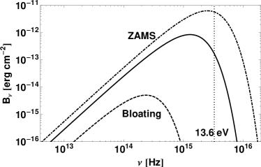
Figure 11: Planck spectra of the protostellar effective surface temperature at the end of the bloating phase (dashed line), after the initial stellar contraction and disk formation (solid line), and at the beginning of the ZAMS (dot-dashed line) in the collapse scenario “RHD+SE A”. The vertical dotted line denotes the hydrogen ionization threshold of 13.6 eV.

Furthermore, the rapid shift of the stellar spectrum depicts a sudden onset of ionization. In the radiation-hydrodynamics evolution of the stellar environment, the effect of ionization is not considered here. For the effects of ionization feedback during the pre-main-sequence evolution of massive stars and implications on observations of H II region variability, we refer the interested reader to recent studies by Peters et al. (2010a, b), and Klassen et al. (2012).

5.4 Phase IV: Main sequence evolution

In the various collapse scenarios, the protostars reach the ZAMS at $21\mbox{ M}_{\odot}$, $30\mbox{ M}_{\odot}$, and $40\mbox{ M}_{\odot}$, respectively. The high stellar masses correspond to lower Kelvin-Helmholtz contraction timescales, leading in general to a decreased dependency of the stellar evolution on the accretion rate. After reaching the ZAMS, the protostellar radius grows along the ZAMS as its mass increases. We stopped the simulation runs shortly after the (proto)star has reached the ZAMS.

6 Aims and limitations

The stellar evolutionary tracks shown here are in reasonably good agreement with previous studies on the evolution of massive protostars including the effect of accretion by Hosokawa & Omukai (2009) and Hosokawa et al. (2010). The initial dominant role of the accretion luminosity, the bloating phase of the protostar, and a smooth transition from the bloating phase towards the ZAMS are robust features in all these studies. However, since the evolution of the protostar will – in general – depend on the initial starting model, we find some differences in the early evolution to the published results by Hosokawa et al. (2010). As an example, the maximum stellar radius during the bloating phase computed here more closely resembles the result by Hosokawa et al. (2010) for their initial condition of a shallower initial entropy distribution (compare Fig. 9 in Hosokawa et al. (2010)), although they assume a much larger initial stellar radius for their starting models. Moreover, the evolution of the protostar depends on the outer boundary condition as well. The outer boundary condition of the stellar evolutionary model is determined by the detailed geometry of the accretion flow onto the stellar surface and how much heat is deposited into the outer stellar layers. In this study, the so-called “cold disk accretion” boundary condition is used, in which the kinetic energy from accretion is assumed to be radiated away without significantly penetrating the stellar atmosphere.

In detail, the protostellar evolution depends on the actual physics of this accretion layer. As an example, we have additionally computed the protostellar evolution for an accretion rate of $\dot{M}=2\times 10^{-3}\mbox{ M}_{\odot}\mbox{ yr}^{-1}$ for cases, in which a fraction of the kinetic accretion energy is absorbed by the protostellar atmospheric layer. In fact, we have studied the limiting and intermediate cases of cold disk accretion ($\eta=0$, the preset model for the previous RHD+SE and SE runs), minor energy absorption ($\eta=10^{-6}$), significant energy absorption ($\eta=0.1$), and full energy absorption ($\eta=1$). The corresponding evolution of the stellar radii and luminosities for these accretion layer scenarios are shown in Fig. 12.

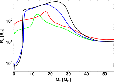
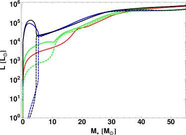
Figure 12: Protostellar radius (upper panel) and luminosities (lower panel) as function of stellar mass for different absorption efficiencies $\eta$ of the accretion energy. The black lines denote the limiting case of $\eta=0$, a so-called cold disk accretion model, in which the kinetic energy from accretion is assumed to be radiated away without significantly penetrating the stellar atmosphere. The blue lines denote the case of $\eta=10^{-6}$. The green lines denote the case of $\eta=0.1$. The red lines denote the limiting case of $\eta=1$, in which the total luminosity of the accreting protostar is just given by its intrinsic stellar luminosity and the accretion energy is fully deposited into the protostellar atmosphere. In the lower panel, solid lines denote the total luminosity including the accretion luminosity and dashed lines denote the intrinsic stellar luminosity only.

In this case of an extremely high accretion rate, the maximum radius of the bloated protostar depends quite strongly on the absorption efficiency $\eta$. While the run of minor energy absorption ($\eta=10^{-6}$) closely resembles the case of cold disk accretion ($\eta=0$), the models for significant ($\eta=0.1$) and full deposition of the accretion energy ($\eta=1$) yield significantly larger radii during the pre-bloated phase and smaller radii during the bloated phase. Eventually, the models merge when the protostar reaches the zero age main sequence.

Our particular choice of the initial model and boundary conditions for the stellar evolution code were not made specifically to quantitatively reproduce any particular previous stellar evolution result. The main goal of this study is to illuminate the interdependencies of protostellar evolution and the evolution of the host molecular core. Thus, to allow comparisons between our self-consistent protostellar evolutionary tracks presented here in three different collapse scenarios, we do not vary the stellar evolution parameters, leaving this type of parameter study for a future investigation. Regarding the hydrodynamical evolution of the proto-stellar environment, we point out that in these axially symmetric studies fragmentation of the forming accretion disk is neglected.

7 Observing bloated massive protostars

Apart from their long distance, observations of massive protostars in general suffer from the fact that the protostars are – especially at these early time in evolution – deeply embedded into their natal environment. On the other hand, due to their high luminosity in combination with a low surface temperature during the bloating phase these massive protostars will have unique signatures. First signs of a strongly bloated, relatively cool central object were reported in an interferometry measurement by Linz et al. (2009). However, this represents an indirect detection due to the fact that the conclusion of a bloated cool object was obtained via a best fit model to the observed data. A second candidate for a massive protostar close to the end of its bloating phase is discussed in (Bik et al. 2012).

To alleviate the extinction problem the best observational chances are given for cases, in which e.g. a protostellar outflow has formed bipolar cavities of low density, which are aligned close to the line of sight. If we assume that the outflow launching is connected to the existence of an accretion disk, this corresponds to an early disk formation scenario such as the collapse scenario “C” herein. The luminosity of the protostar can then be determined by its far infrared spectrum. Measuring the stellar surface temperature is potentially achievable via very high signal to noise ratio K-band spectroscopy. The stellar absorption lines will be heavily veiled by the emission of the circumstellar disk and envelope. These bloated stars will look like red super giants and absorption lines of Mg I and Na I and CO will be observable (Rayner et al. 2009). Another concern arises, if we have in mind that the hot inner rim of the accretion disk can have temperatures comparable to the one of the bloated protostar. Disentangling both temperatures by rotational signatures of the disk material is mostly ruled out due to the fact that we assume to observe the protostar face-on through a low density cavity, forming perpendicular to the accretion disk.

An alternative technique to the one described above is to measure the scattered light in the cavity walls, in case they are not aligned with the line of sight (Testi et al. 2010).

8 Summary and Outlook

We have studied the simultaneous evolution of massive protostars within their evolving host molecular cores. The evolution of the stellar environment is computed with a radiation hydrodynamics code that includes self-gravity and thermal and radiative acceleration feedback. The evolution of the protostar is computed with a stellar evolution code that includes the effects of accretion. The interdependencies of the evolving protostar and molecular core emerge in a variety of phenomena and are studied in three examples of different collapse scenarios: The circumstellar accretion disk forms either prior (collapse scenario “C”), during (collapse scenario “B”), or at the end (collapse scenario “A”) of the protostellar bloating phase.

The protostellar evolutionary tracks calculated here show the robust features of massive protostellar evolution at high accretion rates: Initially, the accretion luminosity dominates over the stellar luminosity. The importance of accretion luminosity decreases with the onset of the bloating phase; the protostar’s radius approaches values up to several $100~{}\mbox{R}_{\odot}$, depending on the accretion rate. After the bloating phase, the protostellar radius decreases until the protostar reaches the ZAMS.

The formation of a circumstellar disk strongly influences the early evolution of the central massive protostar by acting as a “valve” and “low pass filter” for accretion onto the protostar. The disk’s impact strongly depends on the order of events, in particular when the disk is formed with respect to the bloating phase of the star, which itself depends on the initial angular momentum distribution of the local environment. The highest impact on the protostellar evolution occurs, if the disk forms at the end of the bloating phase. The impact is minimal, if the disk forms during the bloating phase.

Approximate evolutionary tracks can provide a reasonable estimate of the protostar’s influence on the molecular environment, if the mean accretion rate onto the protostar is known. In the early phases of evolution this influence is principally the radiation pressure exerted by the new-born protostar. Later, when the massive protostar reaches the ZAMS, the ionizing flux will ionize and heat the surroundings and can ultimately destroy the accretion disk through photoevaporation (Zinnecker & Yorke 2007). Prior to reaching the main sequence, ionization of the surroundings is efficiently suppressed.

It is likely that a number of effects not considered here will contribute to the variability of the accretion rate onto the protostar. We have adopted an “$\alpha$” formalism for angular momentum transfer in the disk (Shakura & Sunyaev 1973). A more precise treatment would necessarily include magnetic fields and the details of their coupling to circumstellar material in a fully three dimensional radiation-magneto-hydrodynamics code. The effects of turbulence, outflows, fragmentation, tidal forces, changes in the abundances of various chemical species and their charged state, gas and dust opacities, and clumpy accretion onto the disk could all lead to increased variability, and some of these processes could both influence and be influenced by protostellar evolution. In this sense, this study should be considered a first step in understanding some of the basic feedback effects of accretion and early protostellar evolution. Further work is needed and will be the subject of future studies.

Finally, with respect to observations, the collapse scenario “C” depicts the most promising example case. The early formation of a circumstellar accretion disk will potentially lead to the launching of a protostellar outflow, which in turn will lead to the formation of low density bipolar cavities. Observations along such cavities (or observations of scattered light at the cavity walls) could lead to the first direct detection of a massive bloated protostar.

Appendix A Additional visualizations

For completeness, we additionally visualize the evolution of the important variables ($R(t),\dot{M}(t)$, and L(t)) with time in Figs. 13 to 21.

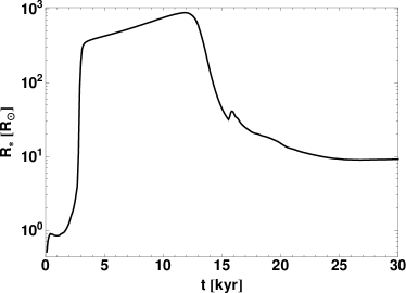
Figure 13: Evolution of the protostellar radius as a function of time in the collapse scenario “RHD+SE A” (solid line).

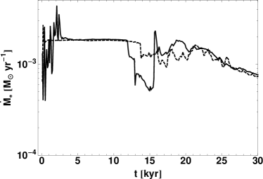
Figure 14: Evolution of the accretion rate as a function of time in the collapse scenario “RHD+SE A” (solid line). The dashed line denotes the evolution of the accretion rate in a comparison run (“RHD A”) using an a priori computed stellar evolutionary track.

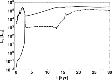
Figure 15: Accretion luminosity (dashed line) and protostellar luminosity (solid line) as a function of time in the collapse scenario “RHD+SE A”.

Figure 16: Evolution of the protostellar radius as a function of time in the collapse scenario “RHD+SE B” (solid line).

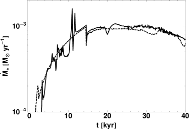
Figure 17: Evolution of the accretion rate as a function of time in the collapse scenario “RHD+SE B” (solid line). The dashed line denotes the evolution of the accretion rate in a comparison run (“RHD B”) using an a priori computed stellar evolutionary track.

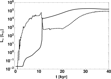
Figure 18: Accretion luminosity (dashed line) and protostellar luminosity (solid line) as a function of time in the collapse scenario “RHD+SE B”.

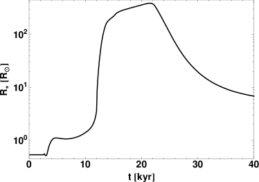
Figure 19: Evolution of the protostellar radius as a function of time in the collapse scenario “RHD+SE C” (solid line).

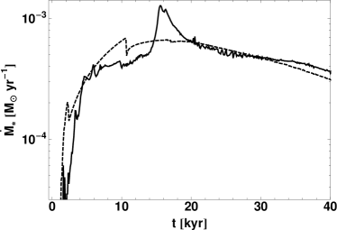
Figure 20: Evolution of the accretion rate as a function of time in the collapse scenario “RHD+SE C” (solid line). The dashed line denotes the evolution of the accretion rate in a comparison run (“RHD C”) using an a priori computed stellar evolutionary track.

Figure 21: Accretion luminosity (dashed line) and protostellar luminosity (solid line) as a function of time in the collapse scenario “RHD+SE C”.

References

- Behrend & Maeder (2001) Behrend, R., & Maeder, A. 2001, A&A, 373, 190
- Beltran et al. (2006) Beltran, M. T., Girart, J. M., & Estalella, R. 2006, A&A, 457, 865
- Beuther et al. (2007) Beuther, H., Churchwell, E. B., McKee, C. F., & Tan, J. C. 2007, in: Protostars and Planets V, ed. B. Reipurth, D. Jewitt, & K. Keil (Tucson, AZ: Univ. Arizona Press), 165
- Beuther et al. (2010) Beuther, H., Linz, H., Bik, A., Goto, M., & Henning, T. 2010, A&A, 512, 29
- Beuther et al. (2002a) Beuther, H., Schilke, P., Gueth, F., McCaughrean, M. J., Andersen, M., Sridharan, T. K., & Menten, K. M. 2002a, A&A, 387, 931
- Beuther et al. (2002b) Beuther, H., Schilke, P., Sridharan, T. K., Menten, K. M., Walmsley, C. M., & Wyrowski, F. 2002b, A&A, 383, 892
- Beuther & Walsh (2008) Beuther, H., & Walsh, A. J. 2008, ApJ, 673, L55
- Beuther et al. (2009) Beuther, H., Walsh, A. J., & Longmore, S. 2009, ApJS, 184, 366
- Beuther et al. (2005) Beuther, H., Zhang, Q., Sridharan, T. K., & Chen, Y. 2005, ApJ, 628, 800
- Bik et al. (2012) Bik, A., Henning, T., Stolte, A., Brandner, W., Gouliermis, D. A., Gennaro, M., Pasquali, A., Rochau, B., Beuther, H., Ageorges, N., Seifert, W., Wang, Y., & Kudryavtseva, N. 2012, ApJ, 744, 87
- Bik et al. (2008) Bik, A., Lenorzer, A., Thi, W. F., Antolin, E. P., Waters, L. B. F. M., Kaper, L., & Martin-Hernández, N. L. 2008, in: Massive Star Formation: Observations Confront Theory, 387, 78
- Bik & Thi (2004) Bik, A., & Thi, W. F. 2004, A&A, 427, L13
- Bodenheimer et al. (2007) Bodenheimer, P., Laughlin, G. P., Rozyczka, M., & Yorke, H. W. 2007, Numerical Methods in Astrophysics: An Introduction. Part of the Series in Astronomy and Astrophysics. Edited by Peter Bodenheimer
- Brooks et al. (2007) Brooks, K. J., Garay, G., Voronkov, M. A., & Rodriguez, L. F. 2007, ApJ, 669, 459
- Cesaroni et al. (1999) Cesaroni, R., Felli, M., Jenness, T., Neri, R., Olmi, L., Robberto, M., Testi, L., & Walmsley, C. M. 1999, A&A, 345, 949
- Cesaroni et al. (1997) Cesaroni, R., Felli, M., Testi, L., Walmsley, C. M., & Olmi, L. 1997, A&A, 325, 725
- Cesaroni et al. (2007) Cesaroni, R., Galli, D., Lodato, G., Walmsley, C. M., & Zhang, Q. 2007, in: Protostars and Planets V, ed. B. Reipurth, D. Jewitt, & K. Keil (Tucson, AZ: Univ. Arizona Press), 197
- Cesaroni et al. (2005) Cesaroni, R., Neri, R., Olmi, L., Testi, L., Walmsley, C. M., & Hofner, P. 2005, A&A, 434, 1039
- Chini et al. (1991) Chini, R. S., Henning, T., & Pfau, W. 1991, A&A, 247, 157
- Chini et al. (2006) Chini, R. S., Hoffmeister, V. H., Nielbock, M., Scheyda, C. M., Steinacker, J., Siebenmorgen, R., & Nürnberger, D. E. A. 2006, ApJ, 645, L61
- Cunningham et al. (2011) Cunningham, A. J., Klein, R. I., Krumholz, M. R., & McKee, C. F. 2011, ApJ, 740, 107
- Dale & Bonnell (2011) Dale, J. E., & Bonnell, I. 2011, MNRAS, 414, 321
- Davis et al. (1998) Davis, C. J., Moriarty-Schieven, G., Eislöffel, J., Hoare, M. G., & Ray, T. P. 1998, ApJ, 115, 1118
- Fallscheer et al. (2009) Fallscheer, C., Beuther, H., Zhang, Q., Keto, E. R., & Sridharan, T. K. 2009, A&A, 504, 127
- Furuya et al. (2008) Furuya, R. S., Cesaroni, R., Takahashi, S., Codella, C., Momose, M., & Beltran, M. T. 2008, ApJ, 673, 363
- Gómez et al. (2003) Gómez, Y., Rodriguez, L. F., Girart, J. M., Garay, G., & Martí, J. 2003, ApJ, 597, 414
- Guzmán et al. (2012) Guzmán, A. E., Garay, G., Brooks, K. J., & Voronkov, M. A. 2012, ApJ, 753, 51
- Harvey et al. (1979) Harvey, P. M., Campbell, M. F., Hoffmann, W. F., Thronson, H. A., & Gatley, I. 1979, ApJ, 229, 990
- Hofner et al. (1999) Hofner, P., Cesaroni, R., Rodriguez, L. F., & Martí, J. 1999, A&A, 345, L43
- Hosokawa & Omukai (2009) Hosokawa, T., & Omukai, K. 2009, ApJ, 691, 823
- Hosokawa et al. (2010) Hosokawa, T., Yorke, H. W., & Omukai, K. 2010, ApJ, 721, 478
- Klassen et al. (2012) Klassen, M., Peters, T., & Pudritz, R. E. 2012, ApJ, 758, 137
- Kraus et al. (2010) Kraus, S., Hofmann, K.-H., Menten, K. M., Schertl, D., Weigelt, G., Wyrowski, F., Meilland, A., Perraut, K., Petrov, R., Robbe-Dubois, S., Schilke, P., & Testi, L. 2010, Nat, 466, 339
- Krumholz et al. (2007) Krumholz, M. R., Klein, R. I., & McKee, C. F. 2007, ApJ, 656, 959
- Krumholz et al. (2009) Krumholz, M. R., Klein, R. I., McKee, C. F., Offner, S. S. R., & Cunningham, A. J. 2009, Science, 323, 754
- Kuiper et al. (2010a) Kuiper, R., Klahr, H., Beuther, H., & Henning, T. 2010a, ApJ, 722, 1556
- Kuiper et al. (2011) —. 2011, ApJ, 732, 20
- Kuiper et al. (2012) —. 2012, A&A, 537, 122
- Kuiper et al. (2010b) Kuiper, R., Klahr, H., Dullemond, C. P., Kley, W., & Henning, T. 2010b, A&A, 511, 81
- Kuiper & Klessen (2013) Kuiper, R., & Klessen, R. S. 2013, eprint arXiv, 1305, 2197
- Leurini et al. (2011) Leurini, S., Codella, C., Zapata, L. A., Beltran, M. T., Schilke, P., & Cesaroni, R. 2011, A&A, 530, 12
- Linz et al. (2009) Linz, H., Henning, T., Feldt, M., Pascucci, I., van Boekel, R., Men’shchikov, A., Stecklum, B., Chesneau, O., Ratzka, T., Quanz, S. P., Leinert, C., Waters, L. B. F. M., & Zinnecker, H. 2009, A&A, 505, 655
- Lyder et al. (1998) Lyder, D. A., Belton, D. S., & Gower, A. C. 1998, ApJ, 116, 840
- Mac Low & Klessen (2004) Mac Low, M.-M., & Klessen, R. S. 2004, Reviews of Modern Physics, 76, 125
- McKee & Ostriker (2007) McKee, C. F., & Ostriker, E. C. 2007, ARA&A, 45, 565
- McKee & Tan (2003) McKee, C. F., & Tan, J. C. 2003, ApJ, 585, 850
- Mignone et al. (2007) Mignone, A., Bodo, G., Massaglia, S., Matsakos, T., Tesileanu, O., Zanni, C., & Ferrari, A. 2007, ApJS, 170, 228
- Nielbock et al. (2007) Nielbock, M., Chini, R. S., Hoffmeister, V. H., Scheyda, C. M., Steinacker, J., Nürnberger, D. E. A., & Siebenmorgen, R. 2007, ApJ, 656, L81
- Palla & Stahler (1991) Palla, F., & Stahler, S. W. 1991, ApJ, 375, 288
- Palla & Stahler (1992) —. 1992, ApJ, 392, 667
- Patel et al. (2005) Patel, N. A., Curiel, S., Sridharan, T. K., Zhang, Q., Hunter, T. R., Ho, P. T. P., Torrelles, J. M., Moran, J. M., Gómez, J. F., & Anglada, G. 2005, Nat, 437, 109
- Peters et al. (2011) Peters, T., Banerjee, R., Klessen, R. S., & Low, M.-M. M. 2011, ApJ, 729, 72
- Peters et al. (2010a) Peters, T., Banerjee, R., Klessen, R. S., Low, M.-M. M., Galvan-Madrid, R., & Keto, E. R. 2010a, ApJ, 711, 1017
- Peters et al. (2010b) Peters, T., Low, M.-M. M., Banerjee, R., Klessen, R. S., & Dullemond, C. P. 2010b, ApJ, 719, 831
- Preibisch et al. (2011) Preibisch, T., Ratzka, T., Gehring, T., Ohlendorf, H., Zinnecker, H., King, R. R., McCaughrean, M. J., & Lewis, J. R. 2011, A&A, 530, 40
- Quanz et al. (2010) Quanz, S. P., Beuther, H., Steinacker, J., Linz, H., Birkmann, S. M., Krause, O., Henning, T., & Zhang, Q. 2010, ApJ, 717, 693
- Rayner et al. (2009) Rayner, J. T., Cushing, M. C., & Vacca, W. D. 2009, ApJS, 185, 289
- Schreyer et al. (2002) Schreyer, K., Henning, T., van der Tak, F. F. S., Boonman, A. M. S., & van Dishoeck, E. F. 2002, A&A, 394, 561
- Schreyer et al. (2006) Schreyer, K., Semenov, D., Henning, T., & Forbrich, J. 2006, ApJ, 637, L129
- Shakura & Sunyaev (1973) Shakura, N. I., & Sunyaev, R. A. 1973, A&A, 24, 337
- Shepherd & Churchwell (1996) Shepherd, D., & Churchwell, E. B. 1996, ApJ, 472, 225
- Sridharan et al. (2005) Sridharan, T. K., Williams, S. J., & Fuller, G. A. 2005, ApJ, 631, L73
- Stahler et al. (1980) Stahler, S. W., Shu, F. H., & Taam, R. E. 1980, ApJ, 242, 226
- Testi et al. (2010) Testi, L., Tan, J. C., & Palla, F. 2010, A&A, 522, 44
- Torrelles et al. (1986) Torrelles, J. M., Ho, P. T. P., Moran, J. M., Rodriguez, L. F., & Canto, J. 1986, ApJ, 307, 787
- Wang et al. (2011) Wang, Y., Beuther, H., Bik, A., Vasyunina, T., Jiang, Z., Puga, E., Linz, H., Rodón, J. A., Henning, T., & Tamura, M. 2011, A&A, 527, 32
- Wheelwright et al. (2012) Wheelwright, H. E., de Wit, W. J., Oudmaijer, R. D., Hoare, M. G., Lumsden, S. L., Fujiyoshi, T., & Close, J. L. 2012, A&A, 540, 89
- Wilking et al. (1989) Wilking, B. A., Blackwell, J. H., Mundy, L. G., & Howe, J. E. 1989, ApJ, 345, 257
- Yorke & Bodenheimer (2008) Yorke, H. W., & Bodenheimer, P. 2008, in: Massive Star Formation: Observations Confront Theory, 387, 189
- Yorke & Sonnhalter (2002) Yorke, H. W., & Sonnhalter, C. 2002, ApJ, 569, 846
- Zhang (2005) Zhang, Q. 2005, in: IAU Symp. Proc. 227, Massive star birth: A crossroads of Astrophysics, ed. R. Cesaroni, M. Felli, E. Churchwell, & C. M. Walmsley (Cambridge: Cambridge Univ. Press), 227, 135
- Zhang et al. (2007) Zhang, Q., Hunter, T. R., Beuther, H., Sridharan, T. K., Liu, S.-Y., Su, Y.-N., Chen, H.-R., & Chen, Y. 2007, ApJ, 658, 1152
- Zhang et al. (2001) Zhang, Q., Hunter, T. R., Brand, J., Sridharan, T. K., Molinari, S., Kramer, M. A., & Cesaroni, R. 2001, ApJ, 552, L167
- Zhang et al. (1998) Zhang, Q., Hunter, T. R., & Sridharan, T. K. 1998, ApJ, 505, L151
- Zinnecker & Yorke (2007) Zinnecker, H., & Yorke, H. W. 2007, ARA&A, 45, 481