Twisted space-time reduced model of large N QCD with two adjoint Wilson fermions

Abstract

The space-time reduced model of large N QCD with two adjoint Wilson fermions is constructed by applying the symmetric twist boundary conditions with non-vanishing flux $k$. For large but finite $N=L^{2}$, the model should behave as the large N version of the ordinary lattice gauge model on a $V=L^{4}$ space-time volume. We perform a comparison of the $N$ dependence of several quantities in this model and in the $k$=0 model (corresponding to periodic boundary conditions). Although the Z⁴(N) symmetry seems unbroken in all cases, the N-dependence analysis favours the use of the same values of $k$ and $L$ for which the symmetry is also unbroken in the pure gauge case. In particular, the $k=0$ model, studied recently by several authors, shows a large and irregular dependence on $N$ within our region of parameters. This makes this reduced model very impractical for extracting physical information about the large N lattice theory. On the contrary, the model for $N=289=17^{2}$ and large enough $k$ gives consistent results, even for extended observables as Wilson loops $W(R,T)$ up to $R,T$=8, matching the expected behaviour for the lattice model with a $17^{4}$ space-time volume.

HUPD-1303
                                                                                   IFT-UAM/CSIC-13-050
                                                                                   FTUAM-13-8

Space-time reduction is one of the most remarkable properties of large N QCD. Eguchi and Kawai (EK) showed[1] that the Schwinger Dyson equations obeyed by Wilson loops in the large N lattice gauge theory are equivalent to those of the theory defined on one-site, provided that the global Z⁴(N) symmetry of the one-site model is not broken. Soon after, it was realized that the Z⁴(N) symmetry is spontaneously broken in the weak coupling region[2]. To cure this problem, two modified models were proposed. One is the quenched EK model[2] which, however, has recently been shown not to work due to the hidden correlation between quenched phases [3]. The other model is the twisted Eguchi-Kawai (TEK) model[4] proposed by the present authors. The original EK model can be thought as the lattice theory defined on one site with periodic boundary conditions. On the other hand, the TEK model corresponds to a one-site model with ‘t Hooft twisted boundary conditions. Choosing the twist tensor appropriately, one can ensure that the ground state of the model respects enough symmetry to guarantee reduction to work at weak coupling. A particularly attractive choice is to take $N$ to be the square of an integer ($N=L^{2}$), and a twist tensor that maintains the symmetry among the 4 space-time directions. This is called symmetric twist and depends on an integer $k$, which characterizes the flux through each plane. In Ref. [4] we restricted our numerical results to the simplest non-zero value $k=1$. A few years ago, several authors reported signals of symmetry breaking for this version of the model at the intermediate coupling region and for $N>100$ [5, 6, 7]. The interpretation for this phenomenon is that the higher entropy of the Z⁴(N)-breaking vacuum configuration overtakes the energy gap with the Z⁴(N)-symmetric ground state, making the former dominate the path integral. In a recent paper [8] we observed that the problem can be solved by tuning $k$ to be proportional to $L$, as the latter is taken to infinity. This makes the energy gap proportional to $N^{2}$ and can even turn the non-symmetric vacuum unstable. Indeed, all the results obtained with this prescription show no signs of symmetry breaking, despite having reached values of $N$ which are one order of magnitude larger than before. Furthermore, we have recently performed a detailed analysis, based on Wilson loops, of the reduced model and of the gauge theory model on a $32^{4}$ lattice and several values of $N$. Our results show an spectacular agreement for several observables, including the string tension, between the values obtained from the reduced model and the infinite $N$ extrapolation of the lattice gauge theory values [9, 10].

One of the important properties of the twisted reduced model is that it gives information about the size and physical interpretation of the finite $N$ corrections. Studying the $N=L^{2}$ model in perturbation theory, one obtains that the gluon propagator becomes identical to that of the ordinary lattice gauge theory formulated on a finite lattice with volume $V=L^{4}$ [4]. This is the main N-dependence but not the only one. In addition, the structure constants of the group appear as momentum dependent phases. These phases cancel out in planar diagrams. For non-planar diagrams, the phases oscillate very quickly for typical momentum values, since they are proportional to $\bar{k}L$, producing a strong suppression. The integer $\bar{k}$ is defined by the relation $k\bar{k}=1\mod L$. To diminish corrections from this source for low momentum modes, we proposed that the large $N$ limit should be taken with both $k$ and $\bar{k}$ proportional to $L$. A recent analysis carried on for the 2+1 dimensional gauge theory [11, 12] shows that this prescription avoids also instabilities associated to the vacuum polarization (See Ref. [13] for numerical results related to this phenomenon).

Recently, space-time reduced models of large N QCD with adjoint fermions have attracted much attention[14, 15, 16, 17, 18, 19]. It is claimed that, in the presence of adjoint fermions, the Z⁴(N) symmetry of the one-site model is not broken even in the periodic boundary conditions case. However, for reduced models with periodic boundary conditions, there is not such a clear connection between the finite $N$ corrections and the finite volume corrections of the ordinary lattice model. This makes it harder to determine what observables are most affected by finite N corrections, and what is the typical size of these corrections.

The purpose of the present letter is to construct the twisted space-time reduced model of large N QCD with two adjoint Wilson fermions and make a study of its finite $N$ behavior. The perturbative arguments relating the finite $N=L^{2}$ reduced model with the lattice model on an $L^{4}$ volume, extend to the case of non-zero flavours of quarks in the adjoint representation. Our results show that the $N$ dependence of various observables of the model with periodic boundary conditions ($k=0$) is large and even irregular. On the contrary, those obtained for our preferred values of $k$ show a mild dependence. In particular, for $N=289=17^{2}$ and $k=3,5$, it is possible to calculate the Wilson loop $W(R,T)$ up to size $R,T=$8, and the results are consistent with what is expected for the large N theory on a $17^{4}$ lattice.

We start from the lattice action of the SU(N) gauge theory coupled with $N_{f}$ flavours of adjoint Wilson fermions, given by

$$S= -bN\sum_{n}\sum_{\mu\neq\nu=1}^{4}{\rm Tr}\left[V_{n,\mu}V_{n+\mu,\nu}V_{n+\nu,\mu}^{\dagger}V_{n,\nu}^{\dagger}\right]-\sum_{j=1}^{N_{f}}\sum_{n}{\rm Tr}\left[\right.{\bar{\Psi}}_{n}^{j}\Psi_{n}^{j}-$$ (1)

$$\kappa\sum_{\mu=1}^{4}\{{\bar{\Psi}}_{n}^{j}(1-\gamma_{\mu})V_{n,\mu}\Psi_{n+\mu}^{j}V_{n,\mu}^{\dagger}+{\bar{\Psi}}_{n}^{j}(1+\gamma_{\mu})V_{n-\mu,\mu}^{\dagger}\Psi_{n-\mu}^{j}V_{n-\mu,\mu}\}\left.\right]$$

where $b$ is the inverse ’t Hooft coupling on the lattice ($b=1/g^{2}N$). $V_{n,\mu}$ are SU(N) matrices, where $n$ runs over the points of a 4-dimensional lattice and $\mu$ over the directions. The fermionic fields $\Psi_{n}^{j}$ are Grassman-valued $N\times N$ matrices, and transforming by adjoint action of the SU(N) group. The label $j$ runs over the $N_{f}$=2 flavour indices. In addition, these fields have spinor indices which are not explicitly shown.

In Ref. [4] we gave the prescription to construct the twisted reduced model for theories in which the different fields transform in the adjoint representation of the group, which includes the present model. The twisted reduced model can be obtained by applying the following replacement rules:

$$V_{n,\nu} \rightarrow V_{\nu}$$

$$V_{n+\mu,\nu} \rightarrow \Gamma_{\mu}V_{\nu}\Gamma_{\mu}^{\dagger}$$

$$V_{n-\mu,\nu} \rightarrow \Gamma_{\mu}^{\dagger}V_{\nu}\Gamma_{\mu}$$

$$\Psi_{n}^{j} \rightarrow \Psi^{j}$$ (2)

$$\Psi_{n+\mu}^{j} \rightarrow \Gamma_{\mu}\Psi^{j}\Gamma_{\mu}^{\dagger}$$

$$\Psi_{n-\mu}^{j} \rightarrow \Gamma_{\mu}^{\dagger}\Psi^{j}\Gamma_{\mu}.$$

where the four twist matrices $\Gamma_{\mu}$ were first introduced in ref.[4] and satisfy the following algebra:

$$\Gamma_{\nu}\Gamma_{\mu}=z_{\mu\nu}\Gamma_{\mu}\Gamma_{\nu}.$$ (3)

For the symmetric twist case, employed in this letter, we take $N=L^{2}$ with $L$ a positive integer, and

$$z_{\mu\nu}=\exp\left(k\frac{2\pi i}{L}\right),\ \ \ z_{\nu\mu}=z_{\mu\nu}^{*},\ \ \ \mu>\nu$$ (4)

The integer $k$ represents the flux through each plane. To preserve enough symmetry in the weak coupling limit, $k$ and $L$ should be co-prime. We recall that our prescription to preserve the symmetry at intermediate couplings for the pure gauge model [8], is to take both $k$ and $\bar{k}$ (defined earlier) large enough.

After twisted reduction, there remain only four SU(N) matrices $V_{\nu}$ and two adjoint fermionic matrix fields $\Psi^{j}$. Applying the rules (2) to the action (1), we obtain

$$S=\ -bN\sum_{\mu\neq\nu=1}^{4}{\rm Tr}\left[V_{\mu}\Gamma_{\mu}V_{\nu}\Gamma_{\mu}^{\dagger}\Gamma_{\nu}V_{\mu}^{\dagger}\Gamma_{\nu}^{\dagger}V_{\nu}^{\dagger}\right]-\sum_{j=1}^{N_{f}}{\rm Tr}\left[\right.{\bar{\Psi}}^{j}\Psi^{j}$$

$$- \kappa\sum_{\mu=1}^{4}\left\{{\bar{\Psi}}^{j}(1-\gamma_{\mu})V_{\mu}\Gamma_{\mu}\Psi^{j}\Gamma_{\mu}^{\dagger}V_{\mu}^{\dagger}+{\bar{\Psi}}^{j}(1+\gamma_{\mu})\Gamma_{\mu}^{\dagger}V_{\mu}^{\dagger}\Psi^{j}V_{\mu}\Gamma_{\mu}\right\}\left.\right].$$ (5)

Finally, applying the change of variables

$$U_{\mu}=V_{\mu}\Gamma_{\mu}$$ (6)

and using (3), we arrive at

$$S=\ -bN\sum_{\mu\neq\nu=1}^{4}{\rm Tr}\left[z_{\mu\nu}U_{\mu}U_{\nu}U_{\mu}^{\dagger}U_{\nu}^{\dagger}\right]-\sum_{j=1}^{N_{f}}{\rm Tr}\left[\right.{\bar{\Psi}}^{j}\Psi^{j}$$ (7)

$$-\kappa\sum_{\mu=1}^{4}\left\{{\bar{\Psi}}^{j}(1-\gamma_{\mu})U_{\mu}\Psi^{j}U_{\mu}^{\dagger}+{\bar{\Psi}}^{j}(1+\gamma_{\mu})U_{\mu}^{\dagger}\Psi^{j}U_{\mu}\right\}\left.\right]$$

$$\equiv\ -bN\sum_{\mu\neq\nu=1}^{4}{\rm Tr}\left[z_{\mu\nu}U_{\mu}U_{\nu}U_{\mu}^{\dagger}U_{\nu}^{\dagger}\right]-\sum_{j=1}^{N_{f}}{\rm Tr}\left[{\bar{\Psi}}^{j}D_{W}\Psi^{j}\right].$$

in which the twist matrices $\Gamma_{\mu}$ have disappeared completely, and there only remains a $z_{\mu\nu}$ factor in the gauge part of the action.

The action (7) is the final form of the twisted reduced model. Notice that for $k=0$ it becomes identical to the reduced model with periodic boundary conditions ($\Gamma_{\mu}$=I for all $\mu$). The action is invariant under the Z⁴(N) global symmetry $U_{\mu}\rightarrow z_{\mu}U_{\mu}$, with $z_{\mu}\in$Z(N). However, to preserve the equivalence of the reduced model with the original lattice model, it is necessary to ensure that a sufficiently large subgroup of the full group remains unbroken spontaneously. In the pure gauge case the symmetric twist boundary conditions are designed to preserve invariance under the subgroup Z⁴(L) in the weak-coupling limit. To monitor that this subgroup remains unbroken, we always calculate the expectation value of ${\rm Tr}(U_{\mu}^{\ell}$), for $1\leq l\leq(L-1)$, which are the order parameters of the Z⁴(L) symmetry. Indeed, we confirm that, in all the simulations presented here, the quantities $<{\rm Tr}(U_{\mu}^{\ell})>$ are compatible with zero within statistical errors.

In this work we have simulated the previous model for various values of $b$, $\kappa$, $k$ and $N$ using the Hybrid Monte Carlo method. Introducing momenta $P_{\mu}$ conjugate to the link variables $U_{\mu}$ and the pseudofermion field $\phi$, the HMC Hamiltonian reads

$$H=\frac{1}{2}\sum_{\mu}{\rm Tr}(P_{\mu}^{2})-bN\sum_{\mu\neq\nu=1}^{4}{\rm Tr}\left(z_{\mu\nu}U_{\mu}U_{\nu}U_{\mu}^{\dagger}U_{\nu}^{\dagger}\right)+{\rm Tr}(\phi^{\dagger}Q^{-2}\phi)$$ (8)

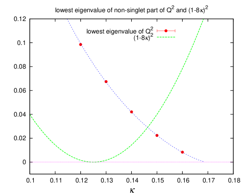
Figure 1: $\kappa$ dependence of the lowest color non-singlet eigenvalue of $Q^{2}$ at $b$=0.35 and $k$=1.

where $Q=D_{W}\gamma_{5}=Q^{\dagger}$ is the hermitian Wilson Dirac matrix and $P_{\mu}$ are traceless $N\times N$ hermitian matrices. $\phi$ is a complex $N\times N$ matrix with implicit Dirac and colour indices (having $4N^{2}$ components). $Q^{2}$ has $4N^{2}$ real and positive eigenvalues. Among them, four degenerate eigenvalues $(1-8\kappa)^{2}$ are related to the unnecessary color singlet component of the $N\otimes{\bar{N}}$ representation. In fig. 1, we plot the lowest color non-singlet eigenvalue of $Q^{2}$ together with $(1-8\kappa)^{2}$ at $b$=0.35 and $k$=1 for several values of $\kappa$. It has been claimed[17] that by imposing ${\rm Tr}\phi$=0, we can reduce the number of CG iterations. This is true if $(1-8\kappa)^{2}$ is smaller than the lowest non-singlet eigenvalues of $Q^{2}$. Otherwise, the color singlet part of $N\otimes{\bar{N}}$ has practically no effect at all. Since our ultimate goal is to study the small quark mass region at large values of $\kappa$, we do not impose the constraint ${\rm Tr}\phi$=0 in our simulations.

We invert $Q^{2}$ using the conjugate gradient (CG) algorithm. Our stopping condition is as follows. Let $r=s-Q^{2}x$ be the residue with $s$ the source. Then we require $|r|^{2}/|s|^{2}<10^{-7}$ during the molecular dynamics evolutions, and $|r|^{2}/|s|^{2}<10^{-15}$ at the global reject-accept step. We always start from $x_{0}$=0 for the initial value of a solution vector to guarantee the reversibility of the trajectories. We use trajectories with unit length, so that the step size $\Delta\tau$ in the molecular dynamics evolution and the number of time steps NMD within one trajectory are inversely connected, $\Delta\tau=$1/NMD. We measure observables every 10 trajectories.

Simulations have been done on Hitachi SR16000 super computer with one node having 32-cores IBM power7 and peak speed of 980 GFlops. Our codes are highly optimized for SR16000 and the sustained speed is 300-600 GFlops depending on the values of $N$ and $\kappa$. The use of this high speed supercomputer enables us to simulate the model up to $N$=289, whereas previous simulations for $k=0$ went only up to $N<50$[15, 17].

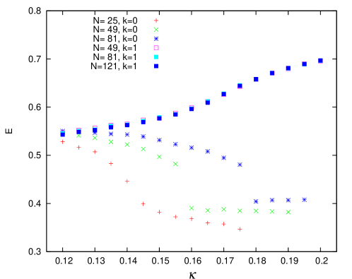
Figure 2: $\kappa$ dependence of the plaquette expectation value $E$ for several values of $N$ at $b$=0.35 and $k$=0 and 1.

Our first analysis focuses on the expectation value of the plaquette
$E=<z_{\mu\nu}\mathrm{Tr}(U_{\mu}U_{\nu}U_{\mu}^{\dagger}U_{\nu}^{\dagger})>$ and its dependence on $\kappa$ and $N$. We first made a rapid scan of the system at $b$=0.35. In fig. 2, we plot the $\kappa$ dependence of the plaquette value $E$ both for $k$=0 and 1 with various values of $N$. For each $N$ and $k$, we start from $\kappa$=0.12 and increase $\kappa$ in steps of 0.005. At each $\kappa$, we run 500 trajectories and make averages using the last 300 trajectories.

For the periodic boundary conditions case $k$=0, the results of our simulations performed at $N$=25, 49 and 81, show that as $\kappa$ increases $E$ decreases, which is quite unnatural. One usually expects to have larger dynamical quark effects as $\kappa$ increases (quark mass decreases). Since the dynamical quark effects tend to order the system, we usually expect to have larger plaquette value $E$ with larger $\kappa$. Notice also that there exists an abrupt change of $E$ at an intermediate value of $\kappa$. The value at which this jump takes place increases by a sizable amount as $N$ grows. Hence, it is clear that this feature should be a finite $N$ artifact. The reason for this behaviour is unclear, but we know that it is not associated to any breaking of the Z⁴(L) symmetry since, as stated earlier, there is no evidence of breaking in all the simulations presented in this paper.

In contrast the $E$ dependence of the twisted $k=1$ model looks very different. In this case the plaquette expectation value $E$ grows with $\kappa$ as expected. Furthermore, the $N$ dependence is much smaller and difficult to see in this rough scale. Notice also that the $k=0$ curves seem to approach the $k=1$ result as $N$ increases. Thus, it is a priori possible that for asymptotic values of $N$ all the curves match.

To understand if this is indeed the case, we made a precise study of the $N$ dependence of the plaquette expectation value $E$ at three fixed values of the parameters ($b$ and $\kappa$) of the action. We chose ($b$, $\kappa$)=(0.35, 0.12), (0.36, 0.12) and (0.35, 0.14). The corresponding results are compiled in tables 1-3. For each run, we use 4000 trajectories, discarding at least the initial 1000 trajectories for thermalization. Errors are estimated by the jack-knife method, splitting up the 4000 trajectories in 10 bins. We choose NMD so as to make the global acceptance ratio larger than 0.5, except for two runs at $b$=0.35 and $\kappa$=0.14. After we started these simulations, we realized that the low acceptance ratio is not due to the small value of NMD, but rather due to the weaker stopping condition $|r|^{2}/|s|^{2}<10^{-7}$. Although a low acceptance ratio does not introduce any systematic error since HMC algorithm is exact, it is desirable to have configuration sets with short autocorrelations. Hence, in the future simulations, needed for the computation of the string tension, we will be able to get higher values of the acceptance ratio.

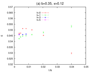
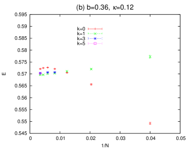
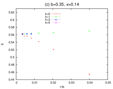
Figure 3: $1/N$ dependence of $E$ for various $k$.

Let us now examine our results. We begin by those obtained at $b$=0.35 and $\kappa$=0.12, presented in table 1 and displayed in fig. 3(a). The results obtained for large $N$ and $k=3$ and $k=5$ are consistent with each other and give a value of $E=$0.5460(2). On the other hand, the results obtained for $k=0$ (periodic boundary conditions) and $k=1$ show an irregular behaviour. For the $k=0$ case, there is first a growth and then a decrease as a function of $N$. Given that $\kappa$ is small, this might be related to the instability of the vacuum for the pure gauge theory. For $k=1$ the instability of the pure gauge theory sets in at $N>100$ [5, 6, 7] and this might also explain the apparent change of tendency present in the data. Indeed, the two smallest values of $N$ for the $k=1$ fall into the line $0.5460+4.47/N^{2}$. However, for larger values of $N$ the value of $E$ does not show signs of stabilizing close to our preferred result. For $k=3$, symmetry breaking for the pure gauge theory sets in at $N>784$, and, if our conjecture is correct, there could be a similar behaviour to be expected at those values of $N$, which are beyond the reach of our computational power. For $k=5$ no breaking has been seen in the pure gauge theory, but according to our arguments of Ref. [8] it should appear for $N>2200$.

In any case, our conclusion is that it is wise to use the same criteria for the model with adjoint fermions as for the pure gauge case since it comes with no additional cost. Namely one has to take $k$ and $L$ coprime, $k/L>0.1$ and with ${\bar{k}}/L$ large enough. Our $k=$3 and 5 results satisfy these criteria.

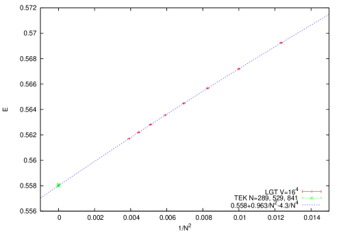
Figure 4: Plaquette expectation value $E$ for the pure gauge case as a function of $1/N^{2}$. The data for $N\leq 16$ are obtained for ordinary lattice gauge theory on a $16^{4}$ lattice. The continuous line shows the result of a fit, which allows the extrapolation to infinite N. On the same plot we also display the value of $E$ obtained for the TEK model at N=841, 529 and 289.

It is interesting to explore what happens at the other values of $b$ and $\kappa$. The results of $(b,\kappa)=(0.36,0.12)$ are collected in table 2 and fig. 3(b), and those of $(b,\kappa)=(0.35,0.14)$ in table 3 and fig. 3(c). At these larger values of $b$ and $\kappa$ things seem to improve for the $k=1$ twisted case and get somewhat worse for the $k=0$ one. For example, if we apply the same criteria to the data at $b=0.36$ as before, the correct result for the plaquette expectation value would be $E=0.5702(1)$. This is essentially the result for $k=5$, while the data of $k=3$ can be fitted to $E=0.5702(1)+9(2)/N^{2}$. If we fit the $k=1$ data for $N<200$ we get $0.5700(2)+4.17/N^{2}$ with a chi square per degree of freedom equal to 1. Indeed, the two largest values of $N$ give a slightly lower value of $0.5696(1)$, probably due to the same problem observed before. On the contrary the $k=0$ has a very strange behaviour. For small $N$, the finite $N$ corrections are huge compared to the twisted case, but then seems to settle at a value of 0.5725(3), although there might be hints that it is starting to decrease. The small difference of $0.002$ in the plaquette value for periodic and twisted boundary conditions might seem worrisome. Our confidence in the level of precision of the twisted result is based on the analysis of the pure gauge case. It is then possible to compare the plaquette expectation value obtained for the twisted Eguchi-Kawai model at b=0.36 with the result of extrapolating the plaquette expectation value for ordinary lattice gauge theory on a $16^{4}$ box (with periodic boundary conditions) and different values of $N$. Indeed, we obtained data for all values of $N$ in the range 9-16 (8 values) with sufficient statistics to achieve a precision of around 0.00002 in all cases. Then we fitted the results to a second degree polynomial in $1/N^{2}$ (3 parameters). The fit is very good with a chi square per degree of freedom of order 1. The best fit gives $E=0.55800(2)+0.963(6)/N^{2}-4.3(4)/N^{4}$. The extrapolated result matches the value obtained for the TEK model for $N=841$ and $k=9$, given by 0.557998(5). Compatible results with larger errors were obtained for $N=$289 with $k=5$ ($E=$0.557991(18)), and 529 with $k=7$ ($E=$0.557989(13)). All the mentioned data and the best fit function are displayed in fig. 4. Statistical errors, also displayed, are too small to be seen on the scale of the figure.

Of course, all the previous information affects the pure gauge model, but there is no reason why the presence of fermions in the adjoint representation should spoil this agreement, but just the opposite.

The data at $b=0.35$, $\kappa=0.14$ confirms the picture. The $k=5$ value is 0.56235(1), the $1/N^{2}$ fit to $k=3$ gives 0.56234(2), and a 3 parameter fit (second degree polynomial in $1/N^{2}$) to the 4 smallest N values of $k=1$ gives 0.5626(3) as large N predictions for the plaquette value. Again the larger values of $N$ for $k=1$ give slightly lower values for the plaquette. The data of $k=0$ shows a very strong and irregular N-dependence, with a similar growth for small N, followed by apparent stabilization and a second growth.

Let us now explore the behaviour of larger Wilson loops. A priori one expects that the finite $N$ corrections grow with the loop size. For the twisted model, as mentioned previously, perturbation theory (and other considerations) relate the finite $N=L^{2}$ theory with the lattice gauge theory at finite volume $L^{4}$. Hence, we expect the corrections to become fairly large when the size of the loop is of the order of $L/2$. If the size is smaller one could obtain reasonably good approximations to the expectation values. For the periodic boundary conditions case $k=0$ it is unclear how these affect the observables with a characteristic lattice scale. In what follows we will present our results which should explore these matters.

In the twisted reduced model, the Wilson loop $W(R,T)$ with size $R\times T$ is calculated from the four link variables $U_{\mu}$ as

$$W(R,T)=z_{\mu\nu}^{RT}<\mathrm{Tr}(U_{\mu}^{R}U_{\nu}^{T}U_{\mu}^{R\dagger}U_{\nu}^{T\dagger})>.$$ (9)

However, Wilson loops are divergent quantities in the continuum limit. One can eliminate constant and perimeter divergences by forming Creutz ratios defined as

$$\chi(R+1/2,T+1/2)=-\log{\frac{W(R+1,T+1)W(R,T)}{W(R+1,T)W(R,T+1)}}.$$ (10)

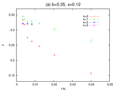
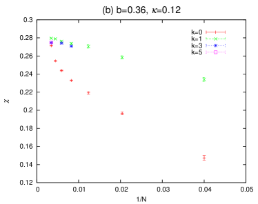
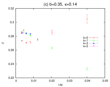
Figure 5: $1/N$ dependence of $\chi$ for various $k$.

Creutz ratios are therefore very important observables, from which one can extract continuum limit quantities, such as the string tension and other continuum functions (See Ref. [9, 10]). Thus, we will start by presenting the $N$ dependence observed in our study for the smallest ratio $\chi(3/2,3/2)$, focusing on the three $(b,\kappa)$ used before for the plaquette. The numerical values appear in the last column of the same tables (1-3) used before. The data is also plotted in fig. 5 to allow for a visual comparison.

The results are in line with our previous findings for the plaquette. The data for $k=3$ and $k=5$ and the various $N$ agree among themselves. For the other values of $k$ the initial trend is towards approaching, but at higher values of $N$ differences are clearly present. The behaviour becomes particularly irregular for $k=0$ and $\kappa=0.14$ for which there is a sudden jump at $N$=225. This strange result might suggest that there are different phases and the system might flip from one to other at different $N$ values.

To study even larger size Wilson loops one has to face the problem that the errors tend to increase considerably. To reduce the fluctuations we will make use of the well-known smearing technique. Here we use the conventional Ape smearing[20]

$$U_{\mu}^{smeared}={\rm Proj}_{N}\left[U_{\mu}+c\sum_{\nu\neq\mu}(z_{\nu\mu}U_{\nu}U_{\mu}U_{\nu}^{\dagger}+z_{\mu\nu}U_{\nu}^{\dagger}U_{\mu}U_{\nu})\right]$$ (11)

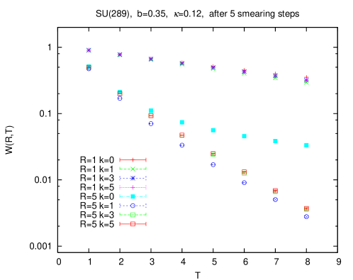
Figure 6: Wilson loop for various values of $k$ after 5 smearing steps.

where ${\rm Proj}_{N}$ stands for the projection operator onto SU(N) matrices. In fig. 6, we show the $k$ dependence of the Wilson loops at $N$=289, $k$=5, $b$=0.35 and $\kappa$=0.12 after 5 smearing steps with the smearing parameter $c$=0.1. For $R$=1, the Wilson loops $W(R=1,T)$ seem to coincide for all $k$ (0, 1, 3 and 5) within such rough scale. For $R$=5, the Wilson loops $W(R=5,T)$ calculated with $k$=3 and 5 agree with each other. According to our previous arguments, they are indeed the correct values of the large N theory. It is amazing that the Wilson loops calculated with the periodic boundary condition ($k$=0) for $T\geq 4$ are so different from those with $k$= 3 and 5 even at $N$=289. The results with $k$=1 are also smaller than those of $k$= 3 and 5.

Finally, we discuss the quark potential defined by

$$V(R,T)=-\log{\frac{W(R,T)}{W(R,T-1)}},$$ (12)

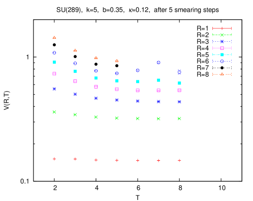
Figure 7: Quark potential $V(R,T)$ after 5 smearing steps.

which is also important from the phenomenological point of view. We expect that for large $T$, $V(R,T)$ tends to $V(R)$, representing the $q{\bar{q}}$ potential at separation $R$. In fig. 7, we show the result of $V(R,T)$ at $N$=289, $k$=5, $b$=0.35, $\kappa$=0.12 after 5 smearing steps. We clearly observe a plateau for large $T$ up to $T$=8 with $R=1\sim 6$. For $R$=7 and 8, we cannot calculate $V(R,T)$ for $T\geq 6$ due to the large noises, but this problem is not specific of the reduced model, since it also appears in ordinary lattice gauge theory. Thus, our results show that, indeed, the reduced model behaves as the large N lattice theory with lattice size $17^{4}$.

In conclusion, in this work we have presented and analyzed the twisted reduced model of large N QCD with two adjoint Wilson fermions. In particular, we focused in studying the $k$ and $N$ dependence of various quantities. Our results show that it is advisable to apply the same criteria in selecting the flux value $k$ as advocated for the pure gauge theory. All the results obtained for that case are perfectly stable with $N$ and behave as expected. For instance, the results for $N$=289 and $k=5$ show that indeed one can compute Wilson loops $W(R,T)$ up to $R,T$=8, in accordance with the association of finite $N$ effects with finite volume effects on a $17^{4}$ lattice. The capacity to explore large loops enables one to estimate the string tension for this theory. Some preliminary results obtained by us have already been reported [21].

The situation for other values of $k$, including periodic boundary conditions, is unclear. Although no symmetry breaking is observed for the range of parameter values explored in this paper, they show large N dependences and anomalous or irregular behaviour for large $N$. The situation is particularly severe for the $k=0$ case. At present, the interpretation is unclear. A recent work [22] suggests that, at least for large values of $b$, the $k=0$ reduced model might fail to match the large N infinite volume theory except for strictly zero mass. It is interesting to point that these problems do not apply for the twisted version with $k\neq 0$. On the contrary, the large $b$ analysis shows that the distribution of eigenvalues is flat, as it should. Our work shows that, even if large N reduction of the $k=0$ model indeed takes place for the region of parameters analyzed in this work, the large N dependences and irregularities presented here seriously limit the applicability of the untwisted version of the reduced model.

Acknowledgements

The authors benefited from interesting conversations with Margarita Garcia Perez, Ken-Ichi Ishikawa, Liam Keegan and Mateusz Koren.

A.G-A is supported from Spanish grants FPA2009-08785, FPA2009-09017, CSD2007-00042, HEPHACOS S2009/ESP-1473, PITN-GA-2009-238353 (ITN STRONGnet), CPAN CSD2007-00042. and the Spanish MINECO Centro de excelencia Severo Ochoa Program under grant SEV-2012-0249. M.O is supported in part by Grants-in-Aid for Scientific Research from the Ministry of Education, Culture, Sports, Science and Technology (No 23540310).

The calculation has been done on Hitachi SR16000-M1 computer at High Energy Accelerator Research Organization (KEK) supported by the Large Scale Simulation Program No.12/13-01 (FY2012-13). The authors thank the Hitachi system engineers for their help in highly optimizing the present simulation code.

$k$	$N$	NMD	acceptance	NCGH	NCGF	$E$	$\chi$
	25	200	0.966	77	44.7	0.52954(73)	0.1572(33)
	49	200	0.919	77	43.7	0.54529(29)	0.2176(15)
	81	200	0.849	75	42.5	0.54966(18)	0.2460(11)
0	121	200	0.725	74	41.6	0.55117(22)	0.2624(7)
	169	200	0.516	73	40.3	0.55122(10)	0.2749(8)
	225	400	0.649	71	36.1	0.54726(11)	0.3175(6)
	289	400	0.544	71	29.9	0.54716(12)	0.3336(4)
	25	200	0.982	54	32.6	0.55319(99)	0.2640(54)
	49	200	0.937	58	34.3	0.54789(61)	0.3023(19)
	81	200	0.871	60	34.9	0.54559(46)	0.3222(18)
1	121	200	0.744	60	34.9	0.54509(23)	0.3286(16)
	169	200	0.542	61	34.0	0.54469(15)	0.3277(11)
	225	400	0.695	62	30.7	0.54392(11)	0.3346(6)
	289	400	0.562	63	25.3	0.54242(12)	0.3452(7)
	121	200	0.742	60	34.8	0.54612(18)	0.3195(10)
3	169	200	0.557	60	33.6	0.54602(15)	0.3209(10)
	289	400	0.567	60	24.0	0.54603(10)	0.3209(4)
5	289	600	0.638	60	24.0	0.54601(10)	0.3215(4)

Table 1: We show several run parameters and observables for the simulations at $b$=0.35 and $\kappa$=0.12. The last two columns list the value of the plaquette $E$ and the Creutz ratio $\chi\equiv\chi(3/2,3/2)$. NMD is the number of time steps within one trajectory and acceptance stands for the global acceptance ratio at reject-accept step. NCGH is the number of CG iterations at global reject-accept step and NCGF is the number of CG iterations during the molecular dynamics evolutions.

$k$	$N$	NMD	acceptance	NCGH	NCGF	$E$	$\chi$
	25	200	0.965	80	46.3	0.54842(63)	0.1473(26)
	49	200	0.917	80	45.3	0.56536(30)	0.1967(16)
	81	200	0.839	79	44.0	0.57046(28)	0.2192(13)
0	121	200	0.720	77	43.2	0.57229(13)	0.2329(6)
	169	200	0.529	76	42.0	0.57268(10)	0.2439(5)
	225	400	0.641	75	38.4	0.57250(10)	0.2546(5)
	289	400	0.520	75	32.2	0.57211(9)	0.2714(5)
	25	200	0.975	55	33.0	0.57666(43)	0.2341(22)
	49	200	0.940	60	35.1	0.57184(35)	0.2584(18)
	81	200	0.862	62	36.0	0.57110(29)	0.2706(19)
1	121	200	0.737	63	36.2	0.57040(15)	0.2738(9)
	169	200	0.540	63	35.5	0.57006(15)	0.2762(8)
	225	400	0.671	64	32.1	0.56964(9)	0.2789(3)
	289	400	0.541	65	26.7	0.56961(9)	0.2796(5)
	121	200	0.731	62	35.9	0.57084(19)	0.2709(5)
3	169	200	0.521	63	34.8	0.57065(15)	0.2742(6)
	289	400	0.535	63	25.4	0.57035(7)	0.2747(4)
5	289	600	0.635	63	25.4	0.57024(5)	0.2749(3)

Table 2: The parameters of the run, the average value of the plaquette $E$ and the Creutz ratio $\chi$ for the simulations at $b$=0.36 and $\kappa$=0.12. The meaning of the headings is the same as in Table 1.

$k$	$N$	NMD	acceptance	NCGH	NCGF	$E$	$\chi$
	25	100	0.928	96	45.6	0.45516(153)	0.3048(64)
	49	100	0.763	110	46.4	0.52043(43)	0.2858(30)
	81	200	0.798	112	44.4	0.54153(38)	0.2755(9)
0	121	300	0.746	111	43.1	0.55135(5)	0.2713(11)
	169	300	0.613	110	41.7	0.55615(10)	0.2705(5)
	225	400	0.532	108	40.1	0.55627(8)	0.2889(4)
	289	500	0.427	108	39.5	0.56059(6)	0.2735(3)
	25	100	0.939	68	35.9	0.56960(82)	0.2330(25)
	49	100	0.796	76	38.4	0.56600(30)	0.2630(16)
	81	100	0.512	80	39.4	0.56420(26)	0.2747(9)
1	121	200	0.667	82	39.6	0.56315(29)	0.2811(7)
	169	300	0.627	83	38.9	0.56206(14)	0.2838(7)
	225	400	0.549	84	37.2	0.56181(11)	0.2857(4)
	289	500	0.468	86	34.9	0.56184(11)	0.2866(4)
	121	200	0.666	81	39.2	0.56260(19)	0.2833(9)
3	169	300	0.629	82	38.6	0.56244(19)	0.2843(4)
	289	500	0.454	82	34.8	0.56239(11)	0.2845(4)
5	289	800	0.500	82	34.8	0.56235(7)	0.2851(4)

Table 3: Run parameters, plaquette value $E$ and Creutz ratio $\chi$ at $b$=0.35 and $\kappa$=0.14. The meaning of run parameters is the same as in Table 1.

References

- [1] T. Eguchi and H. Kawai, Phys. Rev. Lett. 48 (1982) 1004.
- [2] G. Bhanot, U. M. Heller and H. Neuberger, Phys. Lett. B113 (1982) 47.
- [3] B. Bringoltz and S. R. Sharpe, Phys. Rev. D78 (2008) 034507.
- [4] A. Gonzalez-Arroyo and M. Okawa, Phys. Rev. D27 (1983) 2397.
- [5] T. Ishikawa and M. Okawa, talk given at the Annual Meeting of the Physical Society of Japan, March 28-31, Sendai, Japan (2003).
- [6] M. Teper and H. Vairinhos, Phys. Lett. B652 (2007) 359.
- [7] T. Azeyanagi, M. Hanada, T. Hirata and T. Ishikawa, JHEP 0801 (2008) 025.
- [8] A. Gonzalez-Arroyo and M. Okawa, JHEP 1007 (2010) 043.
- [9] A. Gonzalez-Arroyo and M. Okawa, PoS Lattice 2012 (2012) 221.
- [10] A. Gonzalez-Arroyo and M. Okawa, Phys. Lett. B718(2013)1524.
- [11] M. Garcia Perez, A. Gonzalez-Arroyo and M. Okawa, PoS Lattice 2012 (2012) 219.
- [12] M. Garcia Perez, A. Gonzalez-Arroyo and M. Okawa, to appear.
- [13] W. Bietenholz, J. Nishimura, Y. Susaki and J. Volkholz, JHEP 0610 (2006) 042.
- [14] P. Kovtun, M. Unsal, L. G. Yaffe, JHEP 0706 019 (2007) 019.
- [15] T. Azeyanagi, M. Hanada, M. Unsal, R. Yacoby, Phys. Rev. D82 (2010) 125013.
- [16] B. Bringoltz and S. R. Sharpe, Phys. Rev. D80 (2009) 065031.
- [17] B. Bringoltz, M. Koren, S. R. Sharpe, Phys. Rev. D85 (2012) 094504.
- [18] A. Hietanen and R. Narayanan, JHEP 1001 (2010) 079.
- [19] A. Hietanen and R. Narayanan, Phys. Lett. B698 (2011) 171.
- [20] M. Albanese et al. (APE Collaboration), Phys. Lett. B192(1987)163.
- [21] A. Gonzalez-Arroyo and M. Okawa, PoS Lattice 2012 (2012) 046.
- [22] R. Lohmayer and R. Narayanan, arXiv:1305.1279.