Optimal rates of convergence for persistence diagrams in Topological Data Analysis

Abstract

Computational topology has recently known an important development toward data analysis, giving birth to the field of topological data analysis. Topological persistence, or persistent homology, appears as a fundamental tool in this field. In this paper, we study topological persistence in general metric spaces, with a statistical approach. We show that the use of persistent homology can be naturally considered in general statistical frameworks and persistence diagrams can be used as statistics with interesting convergence properties. Some numerical experiments are performed in various contexts to illustrate our results.

1 Introduction

Motivations.

During the last decades, the wide availability of measurement devices and simulation tools has led to an explosion in the amount of available data in almost all domains of Science, industry, economy and even everyday life. Often these data come as point clouds sampled in possibly high (or infinite) dimensional spaces. They are usually not uniformly distributed in the embedding space but carry some geometric structure (manifold or more general stratified space) which reflects important properties of the “systems” from which they have been generated. Moreover, in many cases data are not embedded in Euclidean spaces and come as (finite) sets of points with pairwise distance information. This often happens, for example, with social network or sensor network data where each observation comes with a measure of its distance to the other observations: e.g., in a sensor network distributed in some domain, each sensor may not know its own position, but thanks to the strength of the signal received from the other sensors it may evaluate its distance from them. In such cases data are just given as matrices of pairwise distances between the observations, i.e. as (discrete) metric spaces. Again, although they come as abstract spaces, these data often carry specific topological and geometric structures.

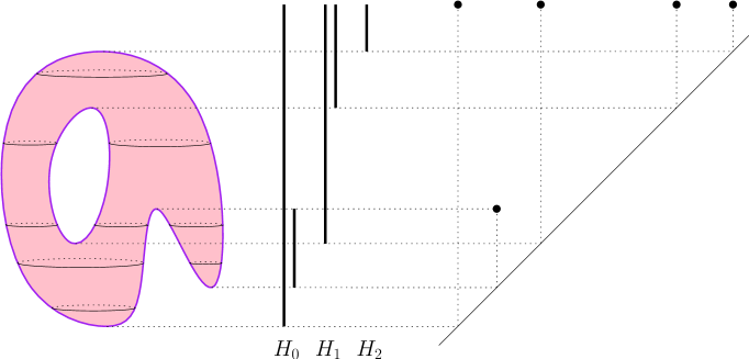
Figure 3: A torus $\mathbb{T}$ filtered by its $z$-coordinate: $\operatorname{\mathrm{Filt}}_{\alpha}=\{P\in\mathbb{T}|P_{z}\leq\alpha\}$, its persistence barcode, and its persistence diagram.

A large amount of research has been done on dimensionality reduction, manifold learning and geometric inference for data embedded in, possibly high dimensional, Euclidean spaces and assumed to be concentrated around low dimensional manifolds; see for instance [42, 44, 31] and the references therein for recent results in this direction. However, the assumption of data lying on a manifold may fail in many applications. In addition, the strategy of representing data by points in Euclidean spaces may introduce large metric distortions as the data may lie in highly curved spaces, instead of in flat Euclidean spaces, raising many difficulties in the analysis of metric data. With the emergence of new geometric inference and algebraic topology tools, computational topology [28] has recently known an important development toward data analysis, giving birth to the field of Topological Data Analysis (TDA) [9] whose aim is to infer multiscale qualitative and quantitative relevant topological structures directly from the data. Topological persistence, more precisely persistent homology appears as a fundamental tool for TDA. Roughly, homology (with coefficient in a field such as, e.g., $\mathbb{Z}/2\mathbb{Z}$) associates to any topological space $\mathbb{M}$, a family of vector spaces (the so-called homology groups) $H_{k}(\mathbb{M})$, $k=0,1,\cdots$, each of them encoding $k$-dimensional features of $\mathbb{M}$. The $k^{th}$ Betti number of $\mathbb{M}$, denoted $\beta_{k}$, is the dimension of $H_{k}(\mathbb{M})$ and measures the number of $k$-dimensional features of $\mathbb{M}$: for example, $\beta_{0}$ is the number of connected components of $\mathbb{M}$, $\beta_{1}$ the number of independent cycles or “tunnels”, $\beta_{2}$ the number of “voids”, etc…; see [32] for a formal introduction to homology. Persistent homology provides a framework [27, 46, 15] and efficient algorithms to encode the evolution of the homology of families of nested topological spaces indexed by a set of real numbers that can often be seen as scale parameters, such as, e.g., the sublevel sets of a function, union of growing balls, etc… The obtained multiscale topological information is then represented in a simple way as a barcode or persistence diagram; see Figure 3 and Section 2.2.
In TDA, persistent homology has found applications in many fields, including neuroscience [41], bioinformatics [33], shape classification [12], clustering [16] and sensor networks [22], to cite just a few. It is usually computed for a filtered simplicial complex built on top of the available data, i.e. a nested family of simplicial complexes whose vertex set is the data set (see Section 2.2). The obtained persistence diagrams are then used as “topological signatures” to exhibit the topological structure underlying the data; see Figure 1. The space of persistence diagrams is endowed with a metric, the so-called bottleneck distance, that allows to compare the obtained signatures and thus to compare the topological structure underlying different data sets. The relevance of this approach relies on stability results ensuring that close data sets, with respect to the so-called Gromov or Gromov-Hausdorff distance, have close persistence diagrams [17, 11, 15, 13]. However these results mainly remain deterministic and thus often restrict to heuristic or exploratory uses in data analysis.

The goal of this paper is to show that, thanks to recent results [15, 13], the use of persistent homology in TDA can be naturally considered in general statistical frameworks and persistence diagrams can be used as statistics with interesting convergence properties.

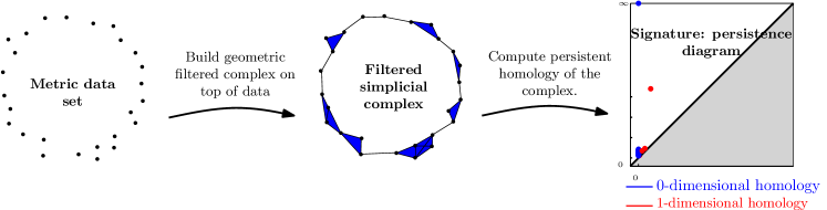
Figure 1: A usual use of persistence in TDA.

Contribution.

In this paper we assume that the available data is the realization of a probability distribution supported on an unknown compact metric space. We consider the persistent homology of different filtered simplicial complexes built on top of the data and we study the rate of convergence of the associated persistence diagrams to some well-defined persistence diagram associated to the support of the probability distribution, with a minimax approach.

More precisely, we assume that we observe a set of $n$ points $\widehat{\mathbb{X}}_{n}=\{X_{1}\dots,X_{n}\}$ in a metric space $(\mathbb{M},\rho)$, drawn i.i.d. from some unknown measure $\mu$ whose support is a compact set denoted $\mathbb{X}_{\mu}\subseteq\mathbb{M}$. We then consider the persistent homology of the filtered simplicial complexes $\operatorname{\mathrm{Filt}}(\mathbb{X}_{\mu})$ and $\operatorname{\mathrm{Filt}}(\widehat{\mathbb{X}})$ built on top of $\mathbb{X}_{\mu}$ and $\widehat{\mathbb{X}}_{n}$ respectively and we establish convergence rates of the bottleneck distance between their persistence diagrams, $\mathrm{d_{b}}\left(\mathsf{dgm}(\operatorname{\mathrm{Filt}}(\mathbb{X}_{\mu})),\mathsf{dgm}(\operatorname{\mathrm{Filt}}(\widehat{\mathbb{X}}))\right)$; see Section 3 for explicit results. It is important to notice that $\mathsf{dgm}(\operatorname{\mathrm{Filt}}(\mathbb{X}_{\mu}))$ encodes topological properties of the support $\mu$ but not of the measure itself. As a consequence, to obtain explicit convergence rates we assume that $\mu$ satisfies the so-called $(a,b)$-standard assumption for some constants $a,b>0$: for any $x\in\mathbb{X}_{\mu}$ and any $r>0$, $\mu(B(x,r))\geq\min(ar^{b},1)$. The following theorem illustrates the kind of results we obtain under such assumption.

Theorem (3.6 in Section 3): Let $(\mathbb{M},\rho)$, $a>0$ and $b>0$ as above. Then for any measure $\mu$ satisfying the $(a,b)$-standard assumption

$$\mathbb{E}\left[\mathrm{d_{b}}(\mathsf{dgm}(\operatorname{\mathrm{Filt}}(\mathbb{X}_{\mu})),\mathsf{dgm}(\operatorname{\mathrm{Filt}}(\widehat{\mathbb{X}}_{n})))\right]\leq C\left(\frac{\ln n}{n}\right)^{1/b}$$

where the constant $C$ only depends on $a$ and $b$ (not on $\mathbb{M}$). Assume moreover that there exists a non isolated point $x$ in $\mathbb{M}$ and consider any sequence $(x_{n})\in\left(\mathbb{M}\setminus\{x\}\right)^{\mathbb{N}}$ such that $\rho(x,x_{n})\leq(an)^{-1/b}$. Then for any estimator $\widehat{\mathsf{dgm}}_{n}$ of $\mathsf{dgm}(\operatorname{\mathrm{Filt}}(\mathbb{X}_{\mu}))$:

$$\liminf_{n\rightarrow\infty}\rho(x,x_{n})^{-1}\mathbb{E}\left[\mathrm{d_{b}}(\mathsf{dgm}(\operatorname{\mathrm{Filt}}(\mathbb{X}_{\mu})),\widehat{\mathsf{dgm}}_{n})\right]\geq C^{\prime}$$

where $C^{\prime}$ is an absolute constant.

Our approach relies on the general theory of persistence modules and our results follow from two recently proven properties of persistence diagrams [13, 11, 15].
First, as $\mathbb{X}_{\mu}$ can be any compact metric space (possibly infinite), the filtered complex $\operatorname{\mathrm{Filt}}(\mathbb{X}_{\mu})$ is usually not finite or even countable and the existence of its persistence diagram cannot be established from the “classical” persistence theory [46, 27]. In our setting, the existence of $\mathsf{dgm}(\operatorname{\mathrm{Filt}}(\mathbb{X}_{\mu}))$ follows from the general persistence framework introduced in [11, 15]. Notice that although this framework is rather abstract and theoretical it does not have any practical drawback as only persistence diagrams of complexes built on top of finite data are computed.
Second, a fundamental property of the persistence diagrams we are considering is their stability proven in [13]: the bottleneck distance between $\mathsf{dgm}(\operatorname{\mathrm{Filt}}(\mathbb{X}_{\mu}))$ and $\mathsf{dgm}(\operatorname{\mathrm{Filt}}(\widehat{\mathbb{X}}_{n}))$ is upper bounded by twice the Gromov-Hausdorff distance between $\mathbb{X}_{\mu}$ and $\widehat{\mathbb{X}}_{n}$. This result establishes a strong connection between our persistence estimation problem and support estimation problems. Upper bounds on the rate of convergence of persistence diagrams are then easily obtained using the same arguments as the ones usually used to obtain convergence results for support estimation with respect to the Hausdorff metric. We take advantage of this general remark to find rates of convergence of persistence diagrams in general metric spaces (Section 3) and also in the more classical case where the measure is supported in $\mathbb{R}^{d}$ (Section 4). Using Le Cam’s lemma, we also compute the corresponding lower bounds to check that the rates of convergence are optimal in the minimax sense.

Related works.

Although it is attracting more and more interest, the use of persistent homology in data analysis remains widely heuristic. There are relatively few papers establishing connections between persistence and statistics and, despite a few promising results, the statistical analysis of homology, persistent homology and more general topological and geometric features of data is still in its infancy.

One of the first statistical results about persistent homology has been given in a parametric setting, by Bubenik and Kim in [6]. They show for instance that for data sampled on an hypersphere according to a von-Mise Fisher distribution (among other distributions), the Betti numbers can be estimated with the parametric rate $n^{-1/2}$. However assuming that both the support and the parametric family of the distribution are known are strong assumptions which are hardly met in practice.

Closely related to our approach, statistical analysis of homology and of persistent homology has also been proposed very recently in [3] and [2] in the specific context of manifolds, i.e. when the geometric structure underlying the data is assumed to be a smooth submanifold of a Euclidean space. In the first paper, the authors exhibit minimax rates of convergence for the estimation of the Betti numbers of the underlying manifold under different models of noise. This approach is also strongly connected to manifold estimation results obtained in [31]. Our results are in the same spirit as [3] but extend to persistent homology and allow to deal with general compact metric spaces. In the second paper, the authors develop several methods to find confidence sets for persistence diagrams using subsampling methods and kernel estimators among other approaches. Although they tackle a different problem, it has some connections with the problem considered in the present paper that we briefly mention in Section 3.4.

Both [2] and our work start from the observation that persistence diagram inference is strongly connected to the better known problem of support estimation. As far as we know, only few results about support estimation in general metric spaces have been given in the past. An interesting framework is proposed in [23]: in this paper the support estimation problem is tackled using kernel methods. On the other hand, a large amount of literature is available for measure support estimation in $\mathbb{R}^{d}$; see for instance the review in [19] for more details. Note that many results on this topic are given with respect to the volume of symmetric set difference - see for instance [4] and references therein - while in our topological estimation setting we need convergence results for support estimation in Hausdorff metric.

The estimator $\widehat{\mathbb{X}}_{n}=\{X_{1},\dots X_{n}\}$ and the Devroye and Wise estimator [24], $\hat{S}_{n}=\bigcup_{i=1}^{n}\bar{B}(X_{i},\varepsilon_{n})$, where $\bar{B}(x,\varepsilon)$ denotes the closed ball centered at $x$ with radius $\varepsilon$, are both natural estimators of the support. The use of $\hat{S}_{n}$ is particularly relevant when the convergence of the measure of the symmetric set difference is considered but does not provide better results than $\widehat{\mathbb{X}}_{n}$ in our Hausdorff distance setting. The convergence rate of $\widehat{\mathbb{X}}_{n}$ to the support of the measure with respect to the Hausdorff distance is given in [21] in $\mathbb{R}^{d}$. Support estimation in $\mathbb{R}^{d}$ has also been studied under various additional assumptions such as, e.g., convexity assumptions [25, 10, 18] or through boundary fragments estimation [35, 34] just to name a few. Another classical assumption is that the measure has a density with respect to the Lebesgue measure. In this context, plug-in methods based on non parametric estimators of the density have been proposed by [20] and [43]. We consider persistence diagram estimation in the density framework of [40] in Section 4 and show in this particular context that $\widehat{\mathbb{X}}_{n}$ allows us to define a persistence diagram estimator that reaches optimal rates of convergence in the minimax sense.

A few other different methods have also been proposed for topology estimation in non deterministic frameworks such as the ones based upon deconvolution approaches [8, 39]. Several recent attempts have also been made, with completely different approaches, to study statistical persistence diagrams from a statistical point of view, such as [37] that studies probability measures on the space of persistence diagrams or [5] that introduces a functional representation of persistence diagrams, the so-called persistence landscapes, allowing to define means and variance of persistence diagrams. Notice that our results should easily extend to persistence landscapes.

The paper is organized as follows. Background notions and results on metric spaces, filtered simplicial complexes, and persistent homology that are necessary to follow the paper are presented in Section 2. The rates of convergence for the estimation of persistence diagrams in general metric spaces are established in Section 3. We also study these convergence rates in $\mathbb{R}^{d}$ for a few classical problems in Section 4. Some numerical experiments illustrating our results are given in Section 5. All the technical proofs are given in Appendix.

2 Background

2.1 Measured metric spaces

Recall that a metric space is a pair $(\mathbb{M},\rho)$ where $\mathbb{M}$ is a set and $\rho:\mathbb{M}\times\mathbb{M}\to\mathbb{R}$ is a nonnegative map such that for any $x,y,z\in\mathbb{M}$, $\rho(x,y)=0$ if and only if $x=y$, $\rho(x,y)=\rho(y,x)$ and $\rho(x,z)\leq\rho(x,y)+\rho(y,z)$. We denote by $\mathcal{K}(\mathbb{M})$ the set of all the compact subsets of $\mathbb{M}$. For a point $x\in\mathbb{M}$ and a subset $C\in\mathcal{K}(\mathbb{M})$, the distance $d(x,C)$ of $x$ to $C$ is the minimum over all $y\in C$ of $d(x,y)$. The Hausdorff distance $\mathrm{d_{\textrm{\tiny H}}}(C_{1},C_{2})$ between two subsets $C_{1},C_{2}\in\mathcal{K}(\mathbb{M})$ is the maximum over all points in $C_{1}$ of their distance to $C_{2}$ and over all points in $C_{2}$ of their distance to $C_{1}$ :

$$\mathrm{d_{\textrm{\tiny H}}}(C_{1},C_{2})=\max\{\,\sup_{x\in C_{1}}d(x,C_{2}),\,\sup_{y\in C_{2}}d(y,C_{1})\,\}.$$

Note that $(\mathcal{K}(\mathbb{M}),\mathrm{d_{\textrm{\tiny H}}})$ is a metric space and can be endowed with its Borel $\sigma$-algebra.

Two compact metric spaces $(\mathbb{M}_{1},\rho_{1})$ and $(\mathbb{M}_{2},\rho_{2})$ are isometric if there exists a bijection $\Phi:\mathbb{M}_{1}\to\mathbb{M}_{2}$ that preserves distances, namely: $\forall x,y\in\mathbb{M}_{1}$, $\rho_{2}(\Phi(x),\Phi(y))=\rho_{1}(x,y)$. Such a map $\Phi$ is called an isometry. One way to compare two metric spaces is to measure how far these two metric spaces are from being isometric. The corresponding distance is called the Gromov-Hausdorff distance (see for instance [7]). Intuitively, it is the infimum of their Hausdorff distance over all possible isometric embeddings of these two spaces into a common metric space.

Definition 2.1.

Let $(\mathbb{M}_{1},\rho_{1})$ and $(\mathbb{M}_{2},\rho_{2})$ be two compact metric spaces. The Gromov-Hausdorff distance $\mathrm{d_{\textrm{\tiny GH}}}\left((\mathbb{M}_{1},\rho_{1})\,,\,(\mathbb{M}_{2},\rho_{2})\right)$ is the infimum of the real numbers $r\geq 0$ such that there exist a metric space $(\mathbb{M},\rho)$ and subspaces $C_{1}$ and $C_{2}$ in $\mathcal{K}(\mathbb{M})$ which are isometric to $\mathbb{M}_{1}$ and $\mathbb{M}_{2}$ respectively and such that $\mathrm{d_{\textrm{\tiny H}}}(C_{1},C_{2})<r$. The Gromov-Hausdorff distance $\mathrm{d_{\textrm{\tiny GH}}}$ defines a metric on the space $\mathcal{K}$ of isometry classes of compact metric spaces (see Theorem 7.3.30 in [7]).

Notice that when $\mathbb{M}_{1}$ and $\mathbb{M}_{2}$ are subspaces of a same metric space $(\mathbb{M},\rho)$ then $\mathrm{d_{\textrm{\tiny GH}}}(\mathbb{M}_{1},\mathbb{M}_{2})\leq\mathrm{d_{\textrm{\tiny H}}}(\mathbb{M}_{1},\mathbb{M}_{2})$.

Measure.

Let $\mu$ be a probability measure on $(\mathbb{M},\rho)$ equipped with its Borel algebra. Let $\mathbb{X}_{\mu}$ denote the support of the measure $\mu$, namely the smallest closed set with probability one. In the following of the paper, we will assume that $\mathbb{X}_{\mu}$ is compact and thus $\mathbb{X}_{\mu}\in\mathcal{K}(\mathbb{M})$. Also note that $(\mathbb{X}_{\mu},\rho)\in\mathcal{K}$.

The main assumption we will need in the following of the paper provides a lower bound on the measure $\mu$. We say that $\mu$ satisfies the standard assumption if there exist $a^{\prime}>0$, $r_{0}>0$ and $b>0$ such that

$$\forall x\in\mathbb{X}_{\mu},\ \forall r\in(0,r_{0}),\ \mu(B(x,r))\geq a^{\prime}r^{b}$$ (2.2)

where $B(x,r)$ denotes the open ball of center $x$ and radius $r$ in $\mathbb{M}$. This assumption is popular in the literature about set estimation (see for instance [19]) but it has generally been considered with $b=d$ in $\mathbb{R}^{d}$. Since $\mathbb{X}_{\mu}$ is compact, reducing the constant $a^{\prime}$ to a smaller constant $a$ if necessary, we easily check that assumption (2.2) is equivalent to

$$\forall x\in\mathbb{X}_{\mu},\ \forall r>0,\ \mu(B(x,r))\geq 1\wedge ar^{b}$$ (2.3)

where $x\wedge y$ denotes the minimum between $x$ and $y$. We then say that $\mu$ satisfies the $(a,b)$-standard assumption.

2.2 Simplicial complexes on metric spaces

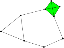
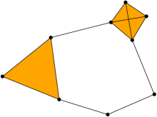
Figure 2: From left to right: the $\alpha$ sublevelset of the distance function to a point set $\mathbb{X}$ in $\mathbb{R}^{2}$, the $\alpha$-complex, $\operatorname{\mathrm{Cech}}_{\alpha}(\mathbb{X})$ and $\operatorname{\mathrm{Rips}}_{2\alpha}(\mathbb{X})$. The last two include a tetrahedron.

Geometric complexes.

The geometric complexes we consider in this paper are built on top of metric spaces and come as nested families depending on a real parameter. Topological persistence is used to infer and encode the evolution of the topology of theses families as the parameter grows. For a complete definition of these geometric filtered complexes built on top of metric spaces and their use in TDA, we refer to [13], Section 4.2. We only give here a brief reminder and refer to Figure 2 for illustrations. A simplicial complex $\mathcal{C}$ is a set of simplexes (points, segments, triangles, etc) such that any face from a simplex in $\mathcal{C}$ is also in $\mathcal{C}$ and the intersection of any two simplices of $\mathcal{C}$ is a (possibly empty) face of these simplices. Notice that we do not assume such simplicial complexes to be finite. The complexes we consider in this paper can be seen as a generalization of neighborhood graphs in dimension larger than $1$.

Given a metric space $\mathbb{X}$ which will also serve as the vertex set, the Vietoris-Rips complex $\operatorname{\mathrm{Rips}}_{\alpha}(\mathbb{X})$ is the set of simplices $[x_{0},\ldots,x_{k}]$ such that $d_{\mathbb{X}}(x_{i},x_{j})\leq\alpha$ for all $(i,j)$. The Čech complex $\operatorname{\mathrm{Cech}}_{\alpha}(\mathbb{X})$ is similarly defined as the set of simplices $[x_{0},\ldots,x_{k}]$ such that the $k+1$ closed balls $B(x_{i},\alpha)$ have a non-empty intersection. Note that these two complexes are related by $\operatorname{\mathrm{Rips}}_{\alpha}(\mathbb{X})\subseteq\operatorname{\mathrm{Cech}}_{\alpha}(\mathbb{X})\subseteq\operatorname{\mathrm{Rips}}_{2\alpha}(\mathbb{X})$. Note also that these two families of complexes only depend on the pairwise distances between the points of $\mathbb{X}$.

When $\mathbb{X}$ is embedded in some larger metric space $\mathbb{M}$, we can extend the definition of the Čech complex to the set of simplices $[x_{0},\ldots,x_{k}]$ such that the $k+1$ closed balls $B(x_{i},\alpha)$ have a non-empty intersection in $\mathbb{M}$ (not just in $\mathbb{X}$). We can also define the alpha-complex or $\alpha$-complex as the set of simplices $[x_{0},\ldots,x_{k}]$ such that, for some $\beta\leq\alpha$ that depends on the simplex, the $k+1$ closed balls $B(x_{i},\beta)$ and the complement of all the other balls $B(x,\beta)$ for $x\in\mathbb{X}$ have a non-empty intersection in $\mathbb{M}$. In the particular case where $\mathbb{M}=\mathbb{R}^{d}$, those two complexes have the same homotopy type (they are equivalent for our purposes) as the union of the balls $B(x,\alpha)$ for $x\in\mathbb{X}$, as in Figure 2, and the $\alpha$-complex only contains simplices of dimension at most $d$. Note that the union of the balls $B(x,\alpha)$ is also the $\alpha$-sublevel set of the distance to $\mathbb{X}$ function $d(.,\mathbb{X})$, and as a consequence, those filtrations thus provide a convenient way to study the evolution of the topology of union of growing balls or sublevel sets of $d(.,\mathbb{X})$ (see Figure 2 and Section 5 for more examples).

There are several other families that we could also have considered, most notably witness complexes [13]. Extending our results to them is straightforward and yields very similar results, so we will restrict to the families defined above in the rest of the paper.

All these families of complexes have the fundamental property that they are non-decreasing with $\alpha$; for any $\alpha\leq\beta$, there is an inclusion of $\operatorname{\mathrm{Rips}}_{\alpha}(\mathbb{X})$ in $\operatorname{\mathrm{Rips}}_{\beta}(\mathbb{X})$, and similarly for the Čech, and Alpha complexes. They are thus called filtrations. In the following, the notation $\operatorname{\mathrm{Filt}}(\mathbb{X}):=(\operatorname{\mathrm{Filt}}_{\alpha}(\mathbb{X}))_{\alpha\in\mathcal{A}}$ denotes one of the filtrations defined above.

Persistence diagrams.

An extensive presentation of persistence diagrams is available in [15]. We recall a few definitions and results that are needed in this paper.

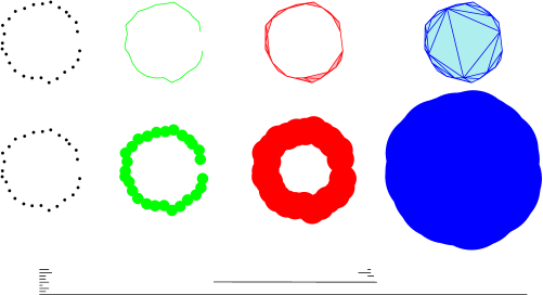
Figure 4: An $\alpha$-complex filtration, the sublevelset filtration of the distance function, and their common persistence barcode (they are homotopy equivalent).

We first give the intuition behind persistence. Given a filtration as above, the topology of $\operatorname{\mathrm{Filt}}_{\alpha}(\mathbb{X})$ changes as $\alpha$ increases: new connected components can appear, existing connected components can merge, cycles and cavities can appear and can be filled, etc. Persistent homology is a tool that tracks these changes, identifies features and associates a lifetime to them. For instance, a connected component is a feature that is born at the smallest $\alpha$ such that the component is present in $\operatorname{\mathrm{Filt}}_{\alpha}(\mathbb{X})$, and dies when it merges with an older connected component. Intuitively, the longer a feature persists, the more relevant it is.

We now formalize the presentation a bit. Given a filtration as above, we can apply the $\mathbb{Z}_{2}$-homology functor and get a sequence of vector spaces $(H(\operatorname{\mathrm{Filt}}_{\alpha}(\mathbb{X})))_{\alpha\in\mathcal{A}}$, where the inclusions $\operatorname{\mathrm{Filt}}_{\alpha}(\mathbb{X})\subseteq\operatorname{\mathrm{Filt}}_{\beta}(\mathbb{X})$ induce linear maps $H(\operatorname{\mathrm{Filt}}_{\alpha}(\mathbb{X}))\rightarrow H(\operatorname{\mathrm{Filt}}_{\beta}(\mathbb{X}))$. In many cases, this sequence can be decomposed as a direct sum of intervals, where an interval is a sequence of the form

$$0\rightarrow\ldots\rightarrow 0\rightarrow\mathbb{Z}_{2}\rightarrow\ldots\rightarrow\mathbb{Z}_{2}\rightarrow 0\rightarrow\ldots\rightarrow 0$$

(the linear maps $\mathbb{Z}_{2}\rightarrow\mathbb{Z}_{2}$ are all the identity). These intervals can be interpreted as features of the (filtered) complex, such as a connected component or a loop, that appear at parameter $\alpha_{\textrm{birth}}$ in the filtration and disappear at parameter $\alpha_{\textrm{death}}$. An interval is determined uniquely by these two parameters. It can be represented as a segment whose extremities have abscissae $\alpha_{\textrm{birth}}$ and $\alpha_{\textrm{death}}$; the set of these segments is called the barcode of $\operatorname{\mathrm{Filt}}(\mathbb{X})$. An interval can also be represented as a point in the plane, where the $x$-coordinate indicates the birth time and the $y$-coordinate the death time. The set of points (with multiplicity) representing the intervals is called the persistence diagram $\mathsf{dgm}(\operatorname{\mathrm{Filt}}(\mathbb{X}))$. Note that the diagram is entirely contained in the half-plane above the diagonal $\Delta$ defined by $y=x$, since death always occurs after birth. [15] shows that this diagram is still well defined even in cases where the sequence might not be decomposable as a finite sum of intervals, and in particular $\mathsf{dgm}(\operatorname{\mathrm{Filt}}(\mathbb{X}))$ is well defined for any compact metric space $\mathbb{X}$ [13]. Note that for technical reasons, the points of the diagonal $\Delta$ are considered as part of every persistence diagram, with infinite multiplicity. The most persistent features (supposedly the most important) are those represented by the longest bars in the barcode, i.e. the points furthest from the diagonal in the diagram, whereas points close to the diagonal can be interpreted as noise.

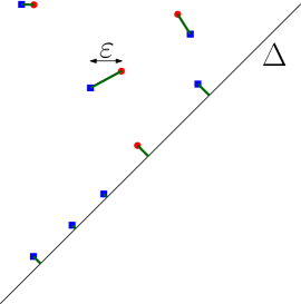
Figure 5: Two diagrams at bottleneck distance $\varepsilon$.

The space of persistence diagrams is endowed with a metric called the bottleneck distance $\mathrm{d_{b}}$. Given two persistence diagrams, it is defined as the infimum, over all perfect matchings of their points, of the largest $L^{\infty}$-distance between two matched points, see Figure 5. The presence of the diagonal in all diagrams means we can consider partial matchings of the off-diagonal points, and the remaining points are matched to the diagonal. With more details, given two diagrams $\mathsf{dgm}_{1}$ and $\mathsf{dgm}_{2}$, we can define a matching $m$ as a subset of $\mathsf{dgm}_{1}\times\mathsf{dgm}_{2}$ such that every point of $\mathsf{dgm}_{1}\setminus\Delta$ and $\mathsf{dgm}_{2}\setminus\Delta$ appears exactly once in $m$. The bottleneck distance is then:

$$\mathrm{d_{b}}(\mathsf{dgm}_{1},\mathsf{dgm}_{2})=\inf_{\textrm{matching }m}\ \max_{(p,q)\in m}\ ||q-p||_{\infty}.$$

Note that points close to the diagonal $\Delta$ are easily matched to the diagonal, which fits with their interpretation as irrelevant noise.

A fundamental property of persistence diagrams, proved in [15], is their stability. If $\mathbb{X}$ and $\tilde{\mathbb{X}}$ are two compact metric spaces then one has

$$\mathrm{d_{b}}\left(\mathsf{dgm}(\operatorname{\mathrm{Filt}}(\mathbb{X})),\mathsf{dgm}(\operatorname{\mathrm{Filt}}(\tilde{\mathbb{X}}))\right)\leq 2\mathrm{d_{\textrm{\tiny GH}}}\left(\mathbb{X},\tilde{\mathbb{X}}\right).$$ (2.4)

Moreover, if $\mathbb{X}$ and $\tilde{\mathbb{X}}$ are embedded in the same metric space $(\mathbb{M},\rho)$ then one has

$$\mathrm{d_{b}}\left(\mathsf{dgm}(\operatorname{\mathrm{Filt}}(\mathbb{X})),\mathsf{dgm}(\operatorname{\mathrm{Filt}}(\tilde{\mathbb{X}}))\right)\leq 2\mathrm{d_{\textrm{\tiny GH}}}\left(\mathbb{X},\tilde{\mathbb{X}}\right)\leq 2\mathrm{d_{\textrm{\tiny H}}}\left(\mathbb{X},\tilde{\mathbb{X}}\right).$$ (2.5)

Notice that these properties are only metric properties: they do not involve here any probability measure on $\mathbb{X}$ and $\tilde{\mathbb{X}}$.

3 Persistence diagrams estimation in metric spaces

Let $(\mathbb{M},\rho)$ be a metric space. Assume that we observe $n$ points $X_{1}\dots,X_{n}$ in $\mathbb{M}$ drawn i.i.d. from some unknown measure $\mu$ whose support is a compact set denoted $\mathbb{X}_{\mu}$.

3.1 From support estimation to persistence diagram estimation

The Gromov-Hausdorff distance allows to compare $\mathbb{X}_{\mu}$ with compact metric spaces not necessarily embedded in $\mathbb{M}$. We thus consider $(\mathbb{X}_{\mu},\rho)$ as an element of $\mathcal{K}$ (rather than an element of $\mathcal{K}(\mathbb{M})$). In the following, an estimator $\widehat{\mathbb{X}}$ of $\mathbb{X}_{\mu}$ is thus a function of $X_{1}\dots,X_{n}$ which takes its values in $\mathcal{K}$ and which is measurable for the Borel algebra induced by $\mathrm{d_{\textrm{\tiny GH}}}$.

Let $\operatorname{\mathrm{Filt}}(\mathbb{X}_{\mu})$ and $\operatorname{\mathrm{Filt}}(\widehat{\mathbb{X}})$ be two filtrations defined on $\mathbb{X}_{\mu}$ and $\widehat{\mathbb{X}}$. The statistical analysis of persistence diagrams proposed in the sequel starts from the following key fact: according to (2.4), for any $\varepsilon>0$:

$$\mathbb{P}\left(\mathrm{d_{b}}\left(\mathsf{dgm}(\operatorname{\mathrm{Filt}}(\mathbb{X}_{\mu})),\mathsf{dgm}(\operatorname{\mathrm{Filt}}(\widehat{\mathbb{X}}))\right)>\varepsilon\right)\leq\mathbb{P}\left(\mathrm{d_{\textrm{\tiny GH}}}(\mathbb{X}_{\mu},\widehat{\mathbb{X}})>2\varepsilon\right)$$ (3.1)

where the probability corresponds to the product measure $\mu^{\otimes n}$. Our strategy then consists in finding an estimator of the support which is close for the $\mathrm{d_{\textrm{\tiny GH}}}$ distance. Note that this general strategy of estimating $\mathbb{X}_{\mu}$ in $\mathcal{K}$ is not only of theoretical interest. Indeed as mentioned in the introduction, in some cases the space $\mathbb{M}$ is unknown and the observations $X_{1}\dots,X_{n}$ are just known through their matrix of pairwise distances $\rho(X_{i},X_{j})$, $i,j=1,\cdots,n$. The use of the Gromov-Hausdorff distance then allows to consider this set of observations as an abstract metric space of cardinality $n$ without taking care of the way it is embedded in $\mathbb{M}$.

This general framework embraces the more standard approach consisting in estimating the support by restraining the values of $\widehat{\mathbb{X}}$ to $\mathcal{K}(\mathbb{M})$. According to (2.5), in this case, for any $\varepsilon>0$:

$$\mathbb{P}\left(\mathrm{d_{b}}\left(\mathsf{dgm}(\operatorname{\mathrm{Filt}}(\mathbb{X}_{\mu})),\mathsf{dgm}(\operatorname{\mathrm{Filt}}(\widehat{\mathbb{X}}))\right)>\varepsilon\right)\leq\mathbb{P}\left(\mathrm{d_{\textrm{\tiny H}}}(\mathbb{X}_{\mu},\widehat{\mathbb{X}})>2\varepsilon\right).$$ (3.2)

Thanks to equations (3.1) and (3.2) the problem of persistence diagrams estimation boils down to the better known problem of estimating the support of a measure.

Let $\widehat{\mathbb{X}}_{n}:=\{X_{1},\dots,X_{n}\}$ be a set of independent observations sampled according to $\mu$ endowed with the restriction of the distance $\rho$. This finite metric space is a natural estimator of the support $\mathbb{X}_{\mu}$. In several contexts discussed in the following, $\widehat{\mathbb{X}}_{n}$ shows optimal rates of convergence for the estimation of $\mathbb{X}_{\mu}$ with respect to the Hausdorff and Gromov-Hausdorff distance. From (3.2) we will then obtain upper bounds on the rate of convergence of $\operatorname{\mathrm{Filt}}(\widehat{\mathbb{X}}_{n})$, and we will need to find the corresponding lower bounds to prove the optimality for topological inference issue.

In the next subsection, we tackle persistence diagram estimation in the general framework of abstract metric spaces. We will consider more particular contexts later in the paper.

3.2 Convergence of persistence diagrams

Cuevas and Rodríguez-Casal give in [21] the rate of convergence in Hausdorff distance of $\widehat{\mathbb{X}}_{n}$ for some probability measure $\mu$ satisfying an $(a,d)$-standard assumption on $\mathbb{R}^{d}$. In this section, we consider the more general context where $\mu$ is a probability measure satisfying an $(a,b)$-standard assumption on a metric space $(\mathbb{M},\rho)$, with $b>0$. We give below the rate of convergence of $\widehat{\mathbb{X}}_{n}$ in this context. The proof follows the lines of the proof of Theorem 3 in [21].

Theorem 3.3.

Assume that a probability measure $\mu$ on $\mathbb{M}$ satisfies the $(a,b)$-standard assumption. Then, for any $\varepsilon>0$:

$$\mathbb{P}\left(\mathrm{d_{\textrm{\tiny H}}}(\mathbb{X}_{\mu},\widehat{\mathbb{X}}_{n})>2\varepsilon\right)\leq\frac{2^{b}}{a\varepsilon^{b}}\exp(-na\varepsilon^{b})\wedge 1.$$

Moreover, there exist two constants $C_{1}$ and $C_{2}$ only depending on $a$ and $b$ such that

$$\limsup_{n\rightarrow\infty}\;\left(\frac{n}{\log n}\right)^{1/b}\mathrm{d_{\textrm{\tiny H}}}(\mathbb{X}_{\mu},\widehat{\mathbb{X}}_{n})\leq C_{1}\hskip 14.22636pt\textrm{ almost surely},$$

and

$$\lim_{n\rightarrow\infty}\;\mathbb{P}\left(\mathrm{d_{\textrm{\tiny H}}}(\mathbb{X}_{\mu},\widehat{\mathbb{X}}_{n})\leq C_{2}\left(\frac{\log n}{n}\right)^{1/b}\right)=1.$$

Since $\mathrm{d_{\textrm{\tiny GH}}}(\mathbb{X}_{\mu},\widehat{\mathbb{X}}_{n})\leq\mathrm{d_{\textrm{\tiny H}}}(\mathbb{X}_{\mu},\widehat{\mathbb{X}}_{n})$ the above theorem also holds when the Gromov distance is replaced by the Gromov-Hausdorff distance. In practice this allows to consider $\widehat{\mathbb{X}}_{n}$ as an abstract metric space without taking care of the way it is embedded in the, possibly unknown, metric space $\mathbb{M}$.

Using (3.1) and (2.5), we then derive from the previous result the following corollary for the convergence rate of the persistence diagram $\operatorname{\mathrm{Filt}}(\widehat{\mathbb{X}}_{n})$ toward $\operatorname{\mathrm{Filt}}(\mathbb{X}_{\mu})$.

Corollary 3.4.

Assume that the probability measure $\mu$ on $\mathbb{M}$ satisfies the $(a,b)$-standard assumption, then for any $\varepsilon>0$:

$$\mathbb{P}\left(\mathrm{d_{b}}\left(\mathsf{dgm}(\operatorname{\mathrm{Filt}}(\mathbb{X}_{\mu})),\mathsf{dgm}(\operatorname{\mathrm{Filt}}(\widehat{\mathbb{X}}_{n}))\right)>\varepsilon\right)\leq\frac{2^{b}}{a\varepsilon^{b}}\exp(-na\varepsilon^{b})\wedge 1.$$ (3.5)

Moreover,

$$\limsup_{n\rightarrow\infty}\;\left(\frac{n}{\log n}\right)^{1/b}\mathrm{d_{b}}\left(\mathsf{dgm}(\operatorname{\mathrm{Filt}}(\mathbb{X}_{\mu})),\mathsf{dgm}(\operatorname{\mathrm{Filt}}(\widehat{\mathbb{X}}_{n}))\right)\leq C_{1}\hskip 14.22636pt\textrm{ almost surely},$$

and

$$\lim_{n\rightarrow\infty}\;\mathbb{P}\left(\mathrm{d_{b}}\left(\mathsf{dgm}(\operatorname{\mathrm{Filt}}(\mathbb{X}_{\mu})),\mathsf{dgm}(\operatorname{\mathrm{Filt}}(\widehat{\mathbb{X}}_{n}))\right)\leq C_{2}\left(\frac{\log n}{n}\right)^{1/b}\right)=1.$$

where $C_{1}$ and $C_{2}$ are the same constants as in Theorem 3.3.

3.3 Optimal rate of convergence

Let $\mathcal{P}(a,b,\mathbb{M})$ be the set of all the probability measures on the metric space $(\mathbb{M},\rho)$ satisfying the $(a,b)$-standard assumption on $\mathbb{M}$.

$$\mathcal{P}(a,b,\mathbb{M}):=\left\{\mu\textrm{ on }\mathbb{M}\>|\>\mathbb{X}_{\mu}\textrm{ is compact and }\forall x\in\mathbb{X}_{\mu},\,\forall r>0,\,\mu\left(B(x,r)\right)\geq 1\wedge ar^{b}\right\}.$$

The next theorem gives upper and lower bounds for the rate of convergence of persistence diagrams. The upper bound comes as a consequence of Corollary 3.4, while the lower bound is established using the so-called Le Cam’s lemma (see Lemma A.1 in Appendix).

Theorem 3.6.

Let $(\mathbb{M},\rho)$ be a metric space and let $a>0$ and $b>0$. Then:

$$\sup_{\mu\in\mathcal{P}(a,b,\mathbb{M})}\mathbb{E}\left[\mathrm{d_{b}}(\mathsf{dgm}(\operatorname{\mathrm{Filt}}(\mathbb{X}_{\mu})),\mathsf{dgm}(\operatorname{\mathrm{Filt}}(\widehat{\mathbb{X}}_{n})))\right]\leq C\left(\frac{\ln n}{n}\right)^{1/b}$$ (3.7)

where the constant $C$ only depends on $a$ and $b$ (not on $\mathbb{M}$). Assume moreover that there exists a non isolated point $x$ in $\mathbb{M}$ and consider any sequence $(x_{n})\in\left(\mathbb{M}\setminus\{x\}\right)^{\mathbb{N}}$ such that $\rho(x,x_{n})\leq(an)^{-1/b}$. Then for any estimator $\widehat{\mathsf{dgm}}_{n}$ of $\mathsf{dgm}(\operatorname{\mathrm{Filt}}(\mathbb{X}_{\mu}))$:

$$\liminf_{n\rightarrow\infty}\rho(x,x_{n})^{-1}\sup_{\mu\in\mathcal{P}(a,b,\mathbb{M})}\,\mathbb{E}\left[\mathrm{d_{b}}(\mathsf{dgm}(\operatorname{\mathrm{Filt}}(\mathbb{X}_{\mu})),\widehat{\mathsf{dgm}}_{n})\right]\geq C^{\prime}$$

where $C^{\prime}$ is an absolute constant.

Consequently, the estimator $\mathsf{dgm}(\operatorname{\mathrm{Filt}}(\widehat{\mathbb{X}}_{n}))$ is minimax optimal on the space $\mathcal{P}(a,b,\mathbb{M})$ up to a logarithmic term as soon as we can find a non-isolated point in $\mathbb{M}$ and a sequence $(x_{n})$ in $\mathbb{M}$ such that $\rho(x_{n},x)\sim(an)^{-1/b}$. This is obviously the case for the Euclidean space $\mathbb{R}^{d}$.

3.4 Confidence sets for persistence diagrams

Corollary 3.4 can also be used to find confidence sets for persistence diagrams. Assume that $a$ and $b$ are known and let $\Psi:\eta\rightarrow\exp(-\eta)/\eta$. Then for $\alpha\in(0,1)$,

$$B_{d_{b}}\left(\mathsf{dgm}(\operatorname{\mathrm{Filt}}(\mathbb{X}_{\mu})),\left[\frac{1}{na}\Psi^{-1}\left(\frac{\alpha}{n2^{b}}\right)\right]^{1/b}\right)$$

is a confidence region for $\mathsf{dgm}\left(\operatorname{\mathrm{Rips}}(\mu(K)\right))$ of level $1-\alpha$. Nevertheless, in practice the coefficients $a$ and $b$ can be unknown. In $\mathbb{R}^{d}$, the coefficient $b$ can be taken equal to the ambient dimension $d$ in many situations. Finding lower bounds on the coefficient $a$ is a tricky problem that is out of the scope of the paper. Alternative solutions have been proposed recently in [2] and we refer the reader to this paper for more details.

4 Persistence diagram estimation in $\boldsymbol{\mathbb{R}^{d}}$

In this section, we study the convergence rates of persistence diagram estimators for data embedded in $\mathbb{R}^{d}$. In particular we study two situations of interest proposed respectively in [40] and [31] in the context of measure support estimation. In the first situation the measure has a density with respect to the Lebesgue measure on $\mathbb{R}^{d}$ whose behavior is controlled near the boundary of its support. In the second case, the measure is supported on a manifold. These two frameworks are complementary and provide realistic frameworks for topological inference in $\mathbb{R}^{d}$.

4.1 Optimal persistence diagram estimation for nonsingular measures on $\mathbb{R}^{d}$

Paper [40] is a significant breakthrough for level set estimation through density estimation. It presents a fully data-driven procedure, in the spirit of Lepski’s method, that is adaptive to unknown local density regularity and achieves a Hausdorff error control that is minimax optimal for a class of level sets with very general shapes. In particular, the assumptions of [40] describe the smoothness of the density near the boundary of the support.

In this section, we propose to study persistence diagram inference in the framework of [40] since this framework is very intuitive and natural. Nevertheless, we do not use the estimator of [40] for this task since we only consider here the support estimation problem (and not the more general level set issue as in [40]). Indeed, we will see that the estimator $\hat{\mathbb{X}}_{n}$ has the optimal rate of convergence for estimating the support according to $\mathrm{d_{\textrm{\tiny H}}}$, as well as for estimating the persistence diagram. We now recall the framework of [40, Section 4.3] corresponding to support set estimation.

Let $X_{1},\dots,X_{n}$ be i.i.d. observations drawn from an unknown probability measure $\mu$ having density $f$ with respect to the Lebesgue measure and defined on a compact set $\chi\subset\mathbb{R}^{d}$. Let $\mathbb{X}_{f}$ denote the support of $\mu$, and let $G_{0}:=\{x\in\chi\>:\>f(x)>0\}$. The boundary of a set $G$ is denoted $\partial G$ and for any $\varepsilon>0$, $I_{\varepsilon}(G):=\bigcup_{x\;|\;B(x,\varepsilon)\subset G}B(x,\varepsilon)$ is the $\varepsilon$-inner of $G$. The two main assumptions of [40] are the following:

$[A]$ : the density $f$ is upper bounded by $f_{\textrm{max}}>0$ and there exist constants $\alpha$, $C_{a}$, $\delta_{a}>0$ such that for all $x\in G_{0}$ with $f(x)\leq\delta_{a}$, $f(x)\geq C_{a}\,d(x,\partial G_{0})^{\alpha}.$

$[B]$ : there exist constants $\varepsilon_{0}>0$ and $C_{b}>0$ such that for all $\varepsilon\leq\varepsilon_{0}$, $I_{\varepsilon}(G_{0})\neq\emptyset$ and $d(x,I_{\varepsilon}(G_{0}))\leq C_{b}\,\varepsilon$ for all $x\in\partial G_{0}$.

We denote by $\mathcal{F}(\alpha)$ the set composed of all the densities on $\chi$ satisfying assumptions $[A]$ and $[B]$, for a fixed set of positive constants $C_{a}$, $C_{b}$, $\delta_{a}$, $\varepsilon_{0}$, $f_{\textrm{max}}$, $p$ and $\alpha$.

Assumption $[A]$ describes how fast the density increases in the neighborhood of the boundary of the support: the smaller $\alpha$, the easier the support may be possible to detect. Assumption $[B]$ prevents the boundary from having arbitrarily small features (as for cusps). We refer to [40] for more details and discussions about these two assumptions and their connections with assumptions in other works.

For persistence diagram estimation, we are interested in estimating the support $\mathbb{X}_{f}$ whereas the assumptions $[A]$ and $[B]$ involve the set $G_{0}$. However, as stated in Lemma B.4 (given in Appendix B.3), these two sets are here almost identical in the sense that $\mathrm{d_{\textrm{\tiny H}}}(G_{0},\mathbb{X}_{f})=0$. Moreover, it can be proved that under assumptions $[A]$ and $[B]$, the measure $\mu$ also satisfies the standard assumption with $b=\alpha+d$ (see Lemma B.4). According to Proposition 3.6, the estimator $\mathsf{dgm}(\operatorname{\mathrm{Filt}}(\widehat{\mathbb{X}}_{n}))$ thus converges in expectation towards $\mathsf{dgm}(\operatorname{\mathrm{Filt}}(\mathbb{X}_{f}))$ with a rate upper bounded by $(\log n/n)^{1/(d+\alpha)}$. We also show that this rate is minimax over the sets $\mathcal{F}(\alpha)$ by adapting the ideas of the proof given in [40] for the Hausdorff lower bound.

Proposition 4.1.

1. For all $n\geq 1$,

   $$sup_{f\in\mathcal{F}(\alpha)}\mathbb{E}\left[\mathrm{d_{b}}(\mathsf{dgm}(\operatorname{\mathrm{Filt}}(\mathbb{X}_{f})),\mathsf{dgm}(\operatorname{\mathrm{Filt}}(\widehat{\mathbb{X}}_{n}))\right]\leq C\left(\frac{n}{\log n}\right)^{-1/(d+\alpha)}$$

   where $C$ is a constant depending only on $C_{a}$, $C_{b}$, $\delta_{a}$, $\varepsilon_{0}$, $f_{\textrm{max}}$, $p$ and $\alpha$.

2. There exists $c>0$ such that

   $$\inf_{\widehat{\mathsf{dgm}}_{n}}\sup_{f\in\mathcal{F}(\alpha)}\mathbb{E}\left[\mathrm{d_{b}}(\mathsf{dgm}(\operatorname{\mathrm{Filt}}(\mathbb{X}_{f})),\widehat{\mathsf{dgm}}_{n})\right]\geq cn^{-1/(d+\alpha)}$$

   for $n$ large enough. The infimum is taken over all possible estimators $\widehat{\mathsf{dgm}}_{n}$ of $\mathsf{dgm}(\operatorname{\mathrm{Filt}}(\mathbb{X}_{f}))$ based on $n$ observations.

Remark.

Paper [40] is more generally about adaptive level set estimation. For this problem, Singh et al. define an histogram based estimator. Let $\mathcal{A}_{j}$ denote the collection of cells, in a regular partition of $\chi=[0,1]^{d}$ into hypercubes of dyadic side length $2^{-j}$. Their estimator $\hat{f}$ is the histogram $\hat{f}(A)=\hat{P}(A)/\mu(A)$, where $\hat{P}(A)=\sum_{i=1\dots n}1_{X_{i}\in A}$. For estimating the level set $G_{\gamma}:=\{x|f(x)\geq\gamma\}$, they consider the estimator

$$\hat{G}_{\gamma,j}=\bigcup_{A\in\mathcal{A}_{j}\;|\;\hat{f}(A)>\gamma}A.$$

It is proved in [40] that $\hat{G}_{\gamma,\hat{j}}$ achieves optimal rates of convergence for estimating the level sets, with $\hat{j}$ chosen in a data driven way. Concerning support estimation, they also show that $\hat{G}_{0,j}$ achieves optimal rates of convergence for estimating $G_{0}$. We have seen that in this context it is also the case for the estimator $\mathbb{X}_{n}$. Since no knowledge of $\alpha$ is required for this last estimator, we thus prefer to use this simpler estimator in this context.

4.2 Optimal rates of convergence of persistence diagram estimation for singular measures in $\mathbb{R}^{D}$

In this subsection, we consider the estimation of the support of a singular measure embedded in $\mathbb{R}^{D}$. A classical assumption in this context is to suppose that the support of the singular measure is a Riemannian manifold. As far as we know, rates of convergence for manifold estimation, namely for the estimation of the support of a singular probability measure supported on a Riemannian manifold of $\mathbb{R}^{D}$, have only been studied recently in [31] and [30]. These papers assume several noise models, which all could be considered in this context of persistence diagram estimation. However, for the sake of simplicity, we only study here the problem where no additional noise is observed, which is referred as the noiseless model in the first of these two papers. As before, upper bounds given in [31] on the rates of convergence for the support estimation in Hausdorff distance directly provide upper bounds on the rates of convergence of the persistence diagram of the support. Before giving the rates of convergence we first recall and discuss the assumptions of [31].

For any $r>0$ and any set $A\subset\mathbb{R}^{d}$, let $A\oplus\varepsilon:=\bigcup_{a\in A}B(a,r)$. Let $\Delta(\mathbb{X}_{\mu})$ be the largest $r$ such that each point in $\mathbb{X}_{\mu}\oplus r$ has a unique projection onto $\mathbb{X}_{\mu}$, this quantity has been introduced by Federer in [29], it is called reach or condition number in the literature.

For a fixed positive integer $d<D$, for some fixed positive constants $b$, $B$, $\kappa$ and for a fixed compact domain $\chi$ in $\mathbb{R}^{p}$, [31] defines the set of probability measures $\mathcal{H}:=\mathcal{H}(d,A,B,\kappa,\chi)$ on $\chi$ satisfying the two following assumptions:

• $[H_{1}]$ The support of the measure $\mu$ is a compact Riemannian manifold $\mathbb{X}_{\mu}$ (included in $\chi$) of dimension $d$ whose reach satisfies

  $$\Delta(\mathbb{X}_{\mu})\geq\kappa.$$ (4.2)

• $[H_{2}]$ The measure $\mu$ is assumed to have a density $g$ with respect to $d$-dimensional volume measure $vol_{d}$ on $\mathbb{X}_{\mu}$, such that

  $$0<A\leq\inf_{y\in\mathbb{X}_{\mu}}g(y)\leq\sup_{y\in\mathbb{X}_{\mu}}g(y)\leq B<\infty.$$ (4.3)

These two assumptions can be easily connected to the standard assumption. Indeed, according to [38] and using $[H_{1}]$, for all $r\leq\kappa$ there exists some constant $C>0$ such that for any $x\in\mathbb{X}_{\mu}$, we have

$$vol_{d}\left(B(x,r)\cap\mathbb{X}_{\mu}\right) \geq C\left(1-\frac{r^{2}}{4\kappa^{2}}\right)^{d/2}r^{d}$$

$$\geq C^{\prime}r^{d}$$

and the same holds for $\mu$ according to $[H_{2}]$. Thus, if we take $\hat{\mathbb{X}}_{n}$ for estimating the support $\mathbb{X}_{\mu}$ in this context, we then obtain the rate of convergence $(\frac{\log n}{n})^{1/d}$ according to Theorem 3.3. Nevertheless, this rate is not minimax optimal on the spaces $\mathcal{H}$ as shown by Theorem 2 in [31]. Indeed the correct rate is $n^{-2/d}$. For proving this result, [31] proposes some “theoretical” estimator that can not be computed in practice. As far as we know, no usable and optimal estimator has been proposed in the literature for this issue. In consequence, the situation is the same for the estimation of persistence diagrams in this context. The following proposition shows that the optimal rates of convergence for support estimation are the same as for the persistence diagram estimation in this context.

Proposition 4.4.

Assume that we observe an $n$-sample under the previous assumptions, then there exist two constants $C$ and $C^{\prime}$ depending only on $\mathcal{H}$ such that

$$Cn^{-2/d}\leq\inf_{\widehat{\mathsf{dgm}}_{n}}\sup_{\mu\in\mathcal{H}}\mathbb{E}\left[\mathrm{d_{b}}(\mathsf{dgm}(\operatorname{\mathrm{Filt}}(\mathbb{X}_{\mu})),\widehat{\mathsf{dgm}}_{n})\right]\leq C^{\prime}n^{-2/d}$$ (4.5)

where the infimum is taken over all the estimators of the persistence diagram.

Of course this result is only of theoretical interest since it is not based on estimators which are usable in practice.

5 Experiments

A series of experiments were conducted in order to illustrate the behavior of the persistence diagrams under sampling of metric spaces endowed with a probability measure and to compare the convergence performance obtained in practice with the theoretical results obtained in the previous sections.

Spaces and data.

We consider four different metric spaces, denoted $\mathbb{M}_{1}$, $\mathbb{M}_{2}$, $\mathbb{M}_{3}$ and $\mathbb{M}_{4}$ hereafter, that are described below.

• (Lissajous curve in $\mathbb{R}^{2}$): the planar curve with the parametric equations $x(t)=\sin(3t+\pi/2)$, $y(t)=\sin(2t)$, $t\in[0,2\pi]$ (see Figure 6, left). Its metric is the restriction of the Euclidean metric in $\mathbb{R}^{2}$ and it is endowed with the push forward by the parametrization of the uniform measure on the interval $[0,2\pi]$.

• (sphere in $\mathbb{R}^{3}$): the unit sphere in $\mathbb{R}^{3}$ (see Figure 6, center). Its metric is the restriction of the Euclidean metric in $\mathbb{R}^{3}$ and it is endowed with the uniform area measure on the sphere.

• (torus in $\mathbb{R}^{3}$): the torus of revolution in $\mathbb{R}^{3}$ with the parametric equations $x(u,v)=(5+\cos(u))\cos(v)$, $y(u,v)=(5+\cos(u))\sin(v)$ and $z(u,v)=\sin(u)$, $(u,v)\in[0,2\pi]^{2}$ (see Figure 6, right). Its metric is the restriction of the Euclidean metric in $\mathbb{R}^{3}$ and it is endowed with the push forward by the parametrization of the uniform measure on the square $[0,2\pi]^{2}$.

• (rotating shape space): for this space we used a 3D character from the SCAPE database [1] and considered all the images of this character from a view rotating around it. We converted these images in gray color and resized these images to $300\times 400=120,000$ pixels (see Figure 7). Each is then identified with a point in $\mathbb{R}^{120,000}$ where the $i^{th}$ coordinate is the level of gray of the $i^{th}$ pixel. Moreover, we normalized these images by projecting them on the unit sphere in $\mathbb{R}^{120,000}$. The metric space $\mathbb{M}_{4}$ is the obtained subset of the unit sphere with the restriction of the Euclidean metric in $\mathbb{R}^{120,000}$. As it is parametrized by a circular set of views, it is endowed with the push forward of the uniform measure on the circle.

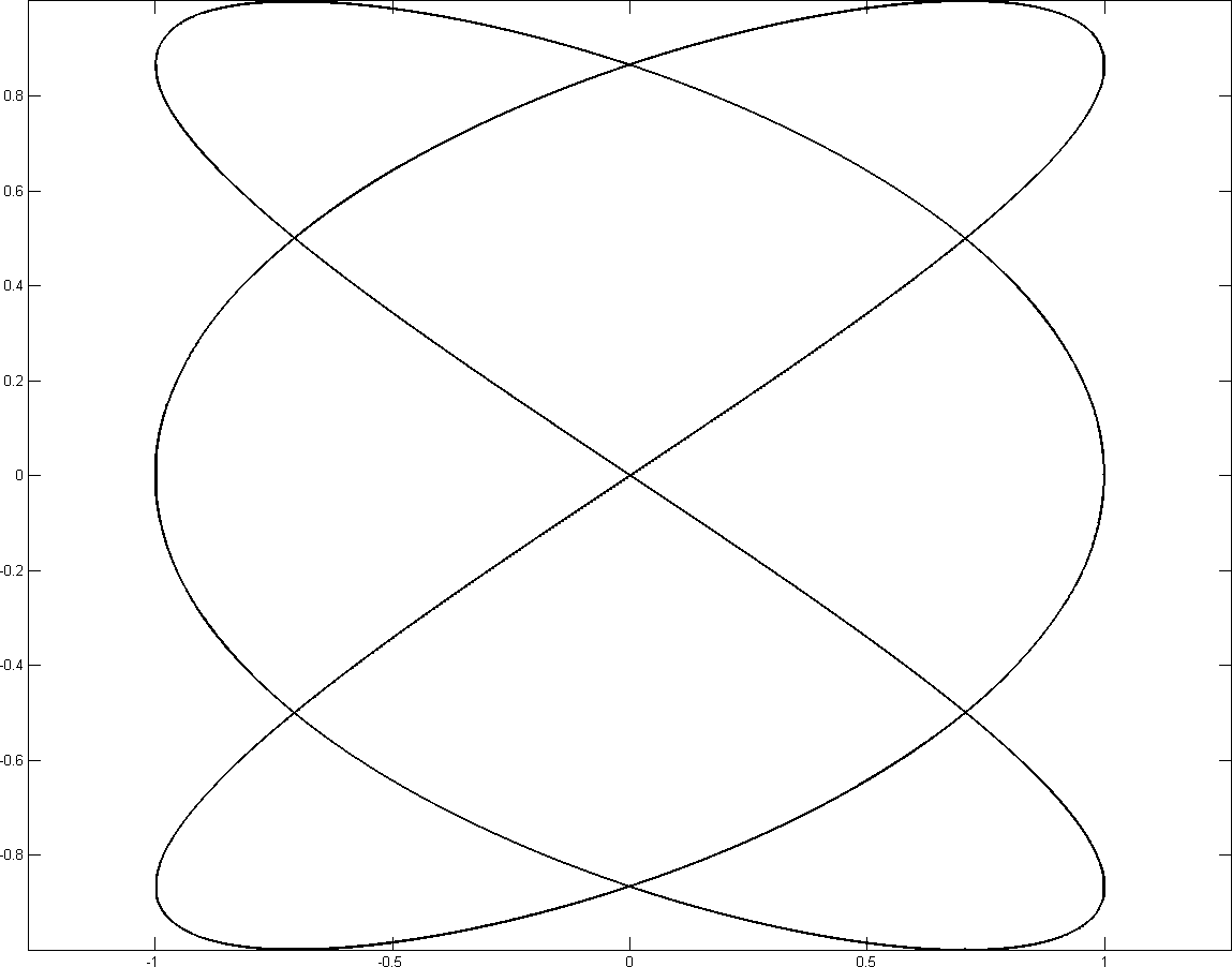
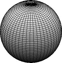
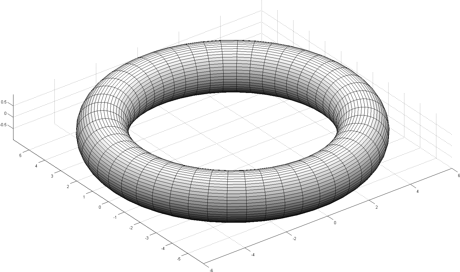
Figure 6: The spaces $\mathbb{M}_{1}$, $\mathbb{M}_{2}$ and $\mathbb{M}_{3}$.

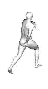
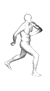
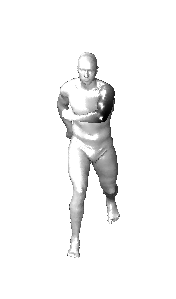
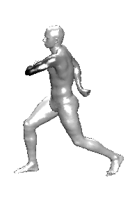
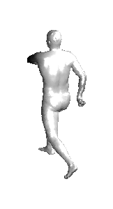
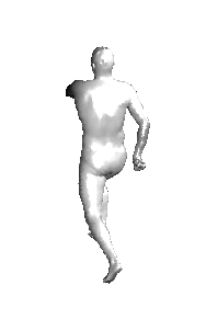
Figure 7: Images sampled from the space $\mathbb{M}_{4}$.

The experiments.

From each of the measured metric spaces $\mathbb{M}_{1}$, $\mathbb{M}_{2}$, $\mathbb{M}_{3}$ and $\mathbb{M}_{4}$ we sampled $k$ sets of $n$ points for different values of $n$ from which we computed persistence diagrams for different geometric complexes (see Table 1). For $\mathbb{M}_{1}$, $\mathbb{M}_{2}$ and $\mathbb{M}_{3}$ we have computed the persistence diagrams for the $1$ or $2$-dimensional homology of the $\alpha$-complex built on top of the sampled sets. As $\alpha$-complexes have the same homotopy type as the corresponding union of balls, these persistence diagrams are the ones of the distance function to the sampled point set [26]. So, for each $n$ we computed the average bottleneck distance between the obtained diagrams and the persistence diagram of the distance to the metric space from which the points were sampled. For $\mathbb{M}_{4}$, as it is embedded in a very high dimensional space, computing the $\alpha$-complex is practically out of reach. So we have computed the persistence diagrams for the $1$-dimensional homology of the Vietoris-Rips complex built on top of the sampled sets. The obtained results are described and discussed below.

• Results for $\mathbb{M}_{1}$: we approximated the $1$-dimensional homology persistence diagram of the distance function to the Lissajous curve $\mathsf{dgm}(\mathbb{M}_{1})$ by sampling $\mathbb{M}_{1}$ with $500,000$ points and computing the persistence diagram of the corresponding $\alpha$-complex. As the Hausdorff distance between our sample and $\mathbb{M}_{1}$ was of order $10^{-5}$ we obtained a sufficiently precise approximation of $\mathsf{dgm}(\mathbb{M}_{1})$ for our purpose. The diagram $\mathsf{dgm}(\mathbb{M}_{1})$ is represented in blue on the left of Figure 8. For each $n$, the average bottleneck distance between $\mathsf{dgm}(\mathbb{M}_{1})$ and the persistence diagrams obtained for the $k=300$ randomly sampled sets $\mathbb{X}_{n}$ of size $n$ has been used as an estimate $\hat{\mathbb{E}}$ of $\mathbb{E}\left[\mathrm{d_{b}}(\mathsf{dgm}(\operatorname{\mathrm{C}_{\alpha}}(\mathbb{M}_{1})),\mathsf{dgm}(\operatorname{\mathrm{C}_{\alpha}}(\widehat{\mathbb{X}}_{n})))\right]$ where $\operatorname{\mathrm{C}_{\alpha}}$ denotes the $\alpha$-complex filtration. $\log(\hat{\mathbb{E}})$ is plotted as a function of $\log(\log(n)/n)$ on Figure 8, right. As expected, since the Lissajous curve is $1$-dimensional, the points are close to a line of slope $1$.

• Results for $\mathbb{M}_{2}$ and $\mathbb{M}_{3}$: the persistence diagrams $\mathsf{dgm}(\mathbb{M}_{2})$ and $\mathsf{dgm}(\mathbb{M}_{2})$ of the distance functions to $\mathbb{M}_{2}$ and $\mathbb{M}_{3}$ are known exactly and are represented in blue on Figures 9 and 10, left, respectively. Notice that we considered the $2$-dimensional homology for $\mathbb{M}_{2}$ and $1$-dimensional homology for $\mathbb{M}_{3}$. For $i=2,3$ and for each $n$, the average bottleneck distance between $\mathsf{dgm}(\mathbb{M}_{i})$ and the persistence diagrams obtained for the $k=100$ randomly sampled sets $\mathbb{X}_{n}$ of size $n$ has been used as an estimate $\hat{\mathbb{E}}$ of $\mathbb{E}\left[\mathrm{d_{b}}(\mathsf{dgm}(\operatorname{\mathrm{C}_{\alpha}}(\mathbb{M}_{i})),\mathsf{dgm}(\operatorname{\mathrm{C}_{\alpha}}(\widehat{\mathbb{X}}_{n})))\right]$ where $\operatorname{\mathrm{C}_{\alpha}}$ denotes the $\alpha$-complex filtration. $\log(\hat{\mathbb{E}})$ is plotted as a function of $\log(\log(n)/n)$ on Figures 9 and 10, right. As expected, since the sphere and the torus are $2$-dimensional, the points are close to a line of slope $1/2$.

• Results for $\mathbb{M}_{4}$: As in that case we do not know the persistence diagram of the Vietoris-Rips filtration built on top of $\mathbb{M}_{4}$, we only computed the $1$-dimensional homology persistence diagrams of the Vietoris-Rips filtrations built on top of $20$ sets of $250$ points each, randomly sampled on $\mathbb{M}_{4}$. All these diagrams have been plotted on the same Figure 11, left. The right of Figure 11 represents a 2D embedding of one of the $250$ points sampled data set using the Multidimensional Scaling algorithm (MDS). Since $\mathbb{M}_{4}$ is a set of images taken according a rotating point of view, it carries a cycle structure. This structure is reflected in the persistence diagrams that all have one point which is clearly off the diagonal. Notice also a second point off the diagonal which is much closer to it and that probably corresponds to the pinching in $\mathbb{M}_{4}$ visible at the bottom left of the MDS projection.

Space	$k$ (sampled sets for each $n$)	$n$ range	Geometric complex
$\mathbb{M}_{1}$	300	$[2100:100:3000]$	$\alpha$-complex
$\mathbb{M}_{2}$	100	$[12000:1000:21000]$	$\alpha$-complex
$\mathbb{M}_{3}$	100	$[4000:500:8500]$	$\alpha$-complex
$\mathbb{M}_{4}$	20	250	Vietoris-Rips complex

Table 1: Sampling parameters and geometric complexes where $[n_{1}:h:n_{2}]$ denotes the set of integers $\{n_{1},n_{1}+h,n_{1}+2h,\cdots n_{2}\}$.

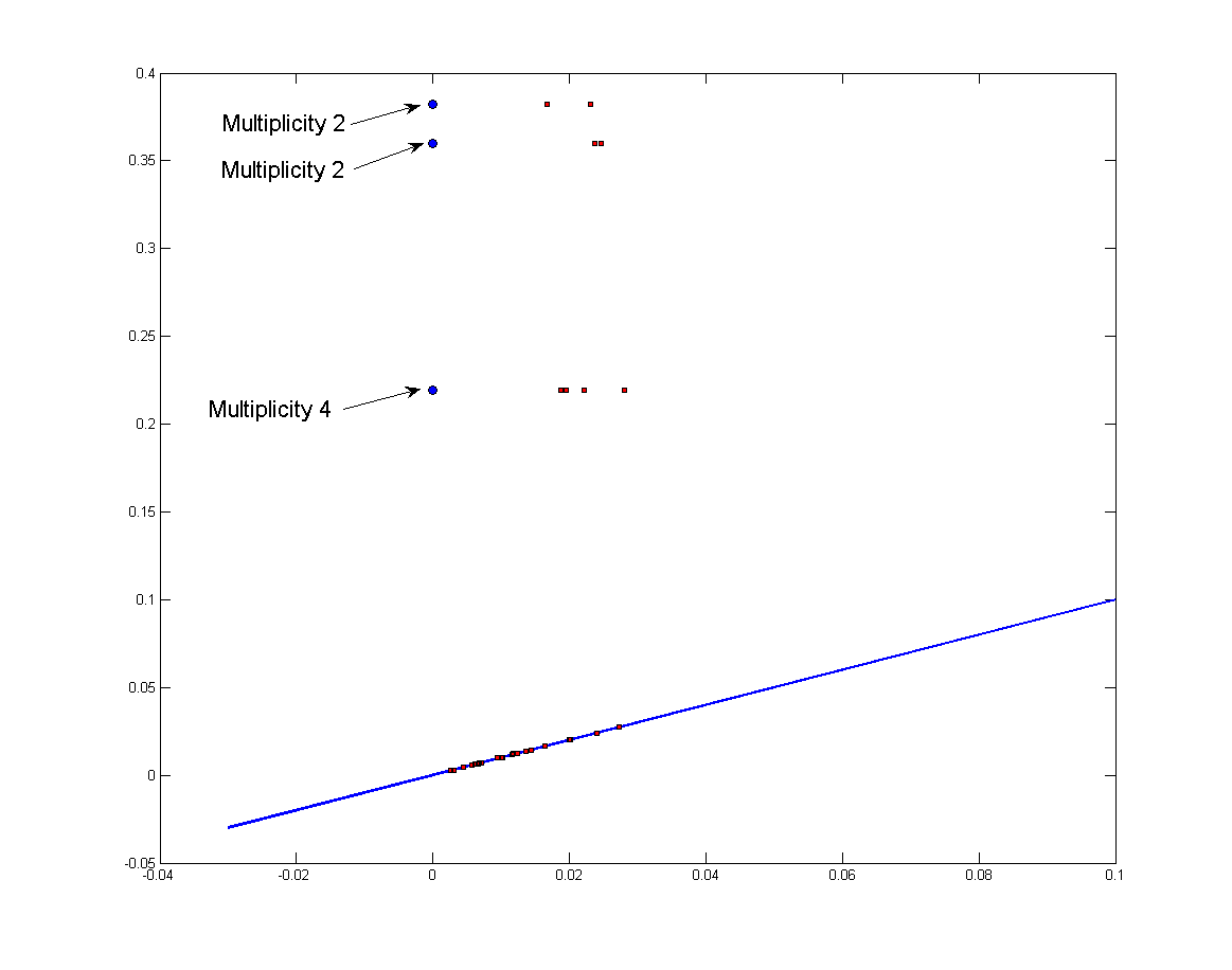
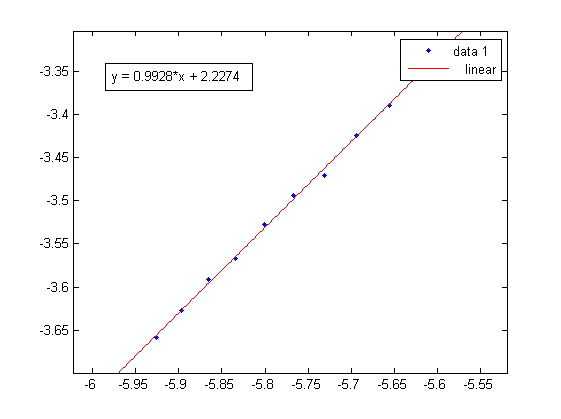
Figure 8: Convergence rate for the persistence diagram of the $\alpha$-filtration built on top of points sampled on $\mathbb{M}_{1}$. Left: in blue the persistence diagram $\mathsf{dgm}(\mathbb{M}_{1})$ of the distance to $\mathbb{M}_{1}$ ($1$-dimensional homology); in red a persistence diagram of the $\alpha$-filtration built on top of $n=2100$ points randomly sampled on $\mathbb{M}_{1}$. Right: the $x$-axis is $\log(\log(n)/n)$ where $n$ is the number of points sampled on $\mathbb{M}_{1}$. The $y$-axis is the $\log$ of the estimated expectation of the bottleneck distance between the diagram obtained from an $\alpha$-filtration built on top of $n$ points sampled on $\mathbb{M}_{1}$ and $\mathsf{dgm}(\mathbb{M}_{1})$.

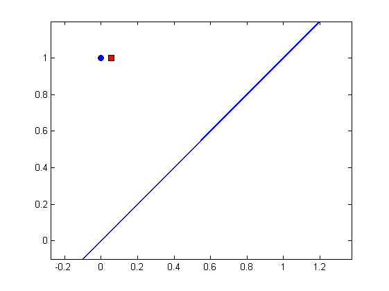
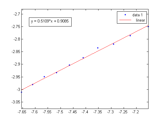
Figure 9: Convergence rate for the persistence diagram of the $\alpha$-filtration built on top of points sampled on $\mathbb{M}_{2}$. Left: in blue the persistence diagram $\mathsf{dgm}(\mathbb{M}_{2})$ of the distance to $\mathbb{M}_{2}$ ($2$-dimensional homology); in red a persistence diagram of the $\alpha$-filtration built on top of $n=12000$ points randomly sampled on $\mathbb{M}_{2}$. Right: the $x$-axis is $\log(\log(n)/n)$ where $n$ is the number of points sampled on $\mathbb{M}_{2}$. The $y$-axis is the $\log$ of the estimated expectation of the bottleneck distance between the diagram obtained from an $\alpha$-filtration built on top of $n$ points sampled on $\mathbb{M}_{2}$ and $\mathsf{dgm}(\mathbb{M}_{2})$.

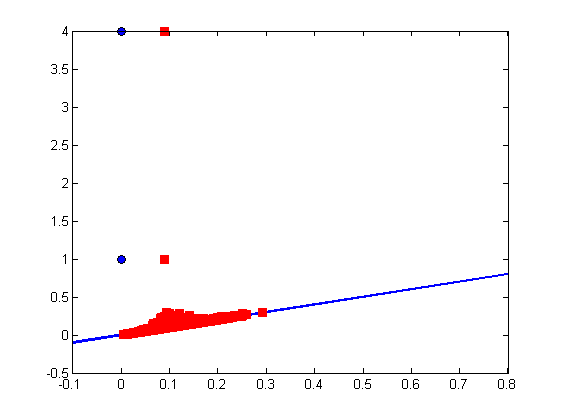
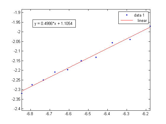
Figure 10: Convergence rate for the persistence diagram of the $\alpha$-filtration built on top of points sampled on $\mathbb{M}_{3}$. Left: in blue the persistence diagram $\mathsf{dgm}(\mathbb{M}_{3})$ of the distance to $\mathbb{M}_{3}$ ($1$-dimensional homology); in red a persistence diagram of the $\alpha$-filtration built on top of $n=14000$ points randomly sampled on $\mathbb{M}_{3}$. Right: the $x$-axis is $\log(\log(n)/n)$ where $n$ is the number of points sampled on $\mathbb{M}_{3}$. The $y$-axis is the $\log$ of the estimated expectation of the bottleneck distance between the diagram obtain from $\alpha$-filtration built on top of $n$ points sampled on $\mathbb{M}_{3}$ and $\mathsf{dgm}(\mathbb{M}_{3})$.

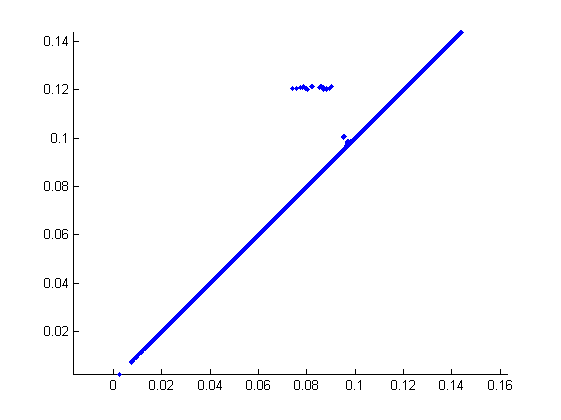
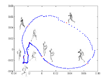
Figure 11: Left: on the same figure the $1$-dimensional homology persistence diagrams of the Vietoris-Rips filtration of $20$ sets of $250$ points sampled on $\mathbb{M}_{4}$. Right: the plot of the embedding of $\mathbb{M}_{4}$ in $\mathbb{R}^{2}$ using MDS.

6 Discussion and future works

In previous works, the use of persistent homology in TDA has been mainly considered with a deterministic approach. As a consequence persistence diagrams were usually used as exploratory tools to analyze the topological structure of data. In this paper, we propose a rigorous framework to study the statistical properties of persistent homology and more precisely we give a general approach to study the rates of convergence for the estimation of persistence diagrams. The results we obtain open the door to a rigorous use of persistence diagrams in statistical framework. Our approach, consisting in reducing persistence diagram estimation to another more classical estimation problem (here support estimation) is based upon recently proven stability results in persistence theory that are very general. As a consequence, our approach can be adapted to other frameworks. For example, the estimation of persistence diagrams of functions (e.g. densities) is strongly connected to the problem of the approximation of such functions with respect to the sup norm. In particular, building on ideas developed in [14] and [8], we intend to extend our results to persistence diagram estimation of distance-to-measure functions and topological inference from data corrupted by different kind of noise.

In another direction, an interesting representation of persistence diagrams as elements of a Hilbert space has recently been proposed in [5]. Our results easily extend to this representation of persistence diagrams called persistence landscapes. Following this promising point of view, we also intend to adapt classical kernel-based methods with kernels carrying topological information.

Appendix A Lecam’s Lemma

The version of Lecam’s Lemma given below is from [45] (see also [30]). Recall that the total variation distance between two distributions $P_{0}$ and $P_{1}$ on a measured space $(\mathcal{X},\mathcal{B})$ is defined by

$$\operatorname{TV}(P_{0},P_{1})=\sup_{B\in\mathcal{B}}|P_{0}(B)-P_{1}(B)|.$$

Moreover, if $P_{0}$ and $P_{1}$ have densities $p_{0}$ and $p_{1}$ for the same measure $\lambda$ on $\mathcal{X}$, then

$$\operatorname{TV}(P_{0},P_{1})=\frac{1}{2}\ell_{1}(p_{0},p_{1}):=\int_{\mathcal{X}}|p_{0}-p_{1}|d\lambda.$$

Lemma A.1.

Let $\mathcal{P}$ be a set of distributions. For $P\in\mathcal{P}$, let $\theta(P)$ take values in a metric space $(\mathbb{X},\rho)$. Let $P_{0}$ and $P_{1}$ in $\mathcal{P}$ be any pair of distributions. Let $X_{1},\dots,X_{n}$ be drawn i.i.d. from some $P\in\mathcal{P}$. Let $\hat{\theta}=\hat{\theta}(X_{1},\dots,X_{n})$ be any estimator of $\theta(P)$, then

$$\sup_{P\in\mathcal{P}}\mathbb{E}_{P^{n}}\rho(\theta,\hat{\theta})\geq\frac{1}{8}\rho\left(\theta(P_{0}),\theta(P_{1})\right)\left[1-\operatorname{TV}(P_{0},P_{1})\right]^{2n}.$$

Appendix B Proofs

B.1 Proof of Theorem 3.3

The proof follows the lines of the proof of Theorem 3 in [21] . The only point to be checked is that the covering number of $\mathbb{X}_{\mu}$ under the $(a,b)$-standard assumption can be controlled as when $b=d\in\mathbb{N}$, the rest of the proof being unchanged.

The covering number $\operatorname{cv}(\mathbb{X}_{\mu},r)$ of $\mathbb{X}_{\mu}$ is the minimum number of balls of radius $r$ that are necessary to cover $\mathbb{X}_{\mu}$:

$$\operatorname{cv}(\mathbb{X}_{\mu},r)=\min\left\{k\in\mathbb{N}^{*}\,:\,\exists(x_{1},\dots,x_{k})\in(\mathbb{X}_{\mu})^{k}\textrm{ such that }\mathbb{X}_{\mu}=\bigcup_{i=1}^{k}B(X_{i},r)\right\}.$$

The packing number $\operatorname{pk}(\mathbb{X}_{\mu},r)$ is the maximum number of balls of radius $r$ that can be packed in $\mathbb{X}_{\mu}$ without overlap:

$$\operatorname{pk}(\mathbb{X}_{\mu},r)=\max\left\{k\in\mathbb{N}^{*}\,:\,\exists(x_{1},\dots,x_{k})\in(\mathbb{X}_{\mu})^{k}\textrm{ such that }B(x_{i},r)\subset\mathbb{X}_{\mu}\textrm{ and }\forall i\not=j\,B(x_{i},r)\cap B(x_{j},r)=\emptyset\right\}$$

The covering and packing numbers are related by the following inequalities (see for instance [36] p.71):

$$\operatorname{pk}(\mathbb{X}_{\mu},2r)\leq\operatorname{cv}(\mathbb{X}_{\mu},2r)\leq\operatorname{pk}(\mathbb{X}_{\mu},r).$$ (B.1)

Lemma B.2.

Assume that the probability $\mu$ satisfies a standard $(a,b)$-assumption. Then for any $r>0$ we have

$$\operatorname{pk}(\mathbb{X}_{\mu},r)\leq\frac{1}{ar^{b}}\vee 1\ \mbox{\rm and}\ \operatorname{cv}(\mathbb{X}_{\mu},r)\leq\frac{2^{b}}{ar^{b}}\vee 1.$$

Proof.

The result is trivial for $r\geq a^{-1/b}$. Let $r<a^{-1/b}$ and let $p=\operatorname{pk}(\mathbb{X}_{\mu},r)$, we choose a maximal packing $B_{1}=B(x_{1},r),\cdots,B_{p}=B(x_{p},r)$ of $\mathbb{X}_{\mu}$. Since the balls of the packing are pairwise disjoint and $\mu$ is a probability measure we have $\sum_{i=1}^{p}\mu(B_{i})\leq 1$. Using that $\mu(B_{i})\geq ar^{b}$ we obtain that $par^{b}\leq\sum_{i=1}^{p}\mu(B_{i})\leq 1$ from which we get the upper bound on $\operatorname{pk}(\mathbb{X}_{\mu},r)$. Since from (B.1) we have $\operatorname{cv}(\mathbb{X}_{\mu},r)\leq\operatorname{pk}(\mathbb{X}_{\mu},r/2)$ we immediately deduce the upper bound on $\operatorname{cv}(\mathbb{X}_{\mu},r)$. ∎

B.2 Proof of Proposition 3.6

Upper bound

We first prove the upper bound. According to Corollary 3.4, thanks to Fubini we have

$$\mathbb{E}\left[\mathrm{d_{b}}(\mathsf{dgm}(\operatorname{\mathrm{Filt}}(\mathbb{X}_{\mu})),\mathsf{dgm}(\operatorname{\mathrm{Filt}}(\widehat{\mathbb{X}}_{n})))\right] \leq \int_{\varepsilon>0}\mathbb{P}\left[\mathrm{d_{b}}(\mathsf{dgm}(\operatorname{\mathrm{Filt}}(\mathbb{X}_{\mu})),\mathsf{dgm}(\operatorname{\mathrm{Filt}}(\widehat{\mathbb{X}}_{n})))>\varepsilon\right]d\varepsilon$$

Let $\varepsilon_{n}=4\left(\frac{\log n}{an}\right)^{1/b}$. By bounding the probability inside this integral by one on $[0,\varepsilon_{n}]$, we find that:

$$\mathbb{E}\left[\mathrm{d_{b}}(\mathsf{dgm}(\operatorname{\mathrm{Filt}}(\mathbb{X}_{\mu})),\mathsf{dgm}(\operatorname{\mathrm{Filt}}(\widehat{\mathbb{X}}_{n})))\right] \leq \varepsilon_{n}+\int_{\varepsilon>\varepsilon_{n}}\frac{8^{b}}{a}\varepsilon^{-b}\exp(-na\varepsilon^{b}/4^{b})d\varepsilon$$

$$\leq \varepsilon_{n}+\frac{4n2^{b}}{b}(na)^{-1/b}\int_{u\geq\log n}u^{1/b-2}\exp(-u)du.$$

Now, if $b\geq\frac{1}{2}$ then $u^{1/b-2}\leq(\log n)^{1/b-2}$ for any $u\geq\log n$ and then

$$\mathbb{E}\left[\mathrm{d_{b}}(\mathsf{dgm}(\operatorname{\mathrm{Filt}}(\mathbb{X}_{\mu})),\mathsf{dgm}(\operatorname{\mathrm{Filt}}(\widehat{\mathbb{X}}_{n})))\right] \leq \varepsilon_{n}+4\frac{2^{b}}{b}\left(\frac{\log n}{n}\right)^{1/b}(\log n)^{-2}$$ (B.3)

$$\leq C_{1}(a,b)\left(\frac{\log n}{n}\right)^{1/b}$$

where the constant $C_{1}(a,b)$ only depends on $a$ and $b$. If $0<b<\frac{1}{2}$, let $p:=\lfloor\frac{1}{b}\rfloor$ and then

$$\int_{u\geq u_{n}:=\log n}u^{1/b-2}\exp(-u)du = u_{n}^{1/b-2}\exp(u_{n})+(\frac{1}{b}-2)u_{n}^{1/b-3}\exp(u_{n})+\dots+$$

$$+\prod_{i=2}^{p}\left(\frac{1}{b}-i\right)u_{n}^{1/b-p}\exp(u_{n})+\int_{u\geq\log n}u^{1/b-p-1}\exp(-u)du$$

$$\leq C_{2}(a,b)\frac{(\log n)^{1/b-2}}{n}$$

where $C_{2}(a,b)$ only depends on $a$ and $b$. Thus (B.3) is also satisfied for $b<\frac{1}{2}$ and the upper bound is proved.

Lower bound

To prove the lower bound, it will be sufficient to consider two Dirac distributions. We take for $P_{0,n}=P_{x}$ the Dirac distribution on $\mathbb{X}_{0}:=\{x\}$ and it is clear that $P_{0}\in\mathcal{P}(a,b,\mathbb{M})$. Let $P_{1,n}$ be the distribution $\frac{1}{n}\delta_{x_{n}}+(1-\frac{1}{n})P_{0}$. The support of $P_{1,n}$ is denoted $\mathbb{X}_{1,n}:=\{x\}\cup\{x_{n}\}$. Note that for any $n\geq 2$ and any $r\leq\rho(x,x_{n})$:

$$P_{1,n}\left(B(x,r)\right)=1-\frac{1}{n}\geq\frac{1}{2}\geq\frac{1}{2\rho(x,x_{n})^{b}}r^{b}\geq ar^{b}$$

and

$$P_{1,n}\left(B(x_{n},r)\right)=\frac{1}{n}=\frac{1}{n\rho(x,x_{n})^{b}}r^{b}\geq ar^{b}.$$

Moreover, for $r>\rho(x,x_{n})$, $P_{1,n}\left(B(0,r)\right)=P_{1,n}\left(B(x_{n},r)\right)=1$. Thus for any $r>0$ and any $x\in\mathbb{X}_{1,n}$:

$$P_{1,n}\left(B(x,r)\right)\geq ar^{b}\wedge 1$$

and $P_{1,n}$ also belongs to $\mathcal{P}(a,b,\mathbb{M})$.

The probability measure $P_{0}$ is absolutely continuous with respect to $P_{1,n}$ and the density of $P_{0}$ with respect to $P_{1,n}$ is $p_{0,n}:=\frac{n}{n-1}\mathbbm{1}_{\{x\}}$. Then

$$TV(P_{0},P_{1,n}) = \int_{\mathbb{M}}|1-\frac{n}{n-1}\mathbbm{1}_{\{x\}}|\;dP_{1,n}$$

$$= \frac{2}{n}.$$

Next, $\left[1-TV(P_{0},P_{1,n})\right]^{2n}=(1-\frac{2}{n})^{2n}\rightarrow e^{-4}$ as $n$ tends to infinity. It remains to compute $\mathrm{d_{b}}(\mathsf{dgm}(\operatorname{\mathrm{Filt}}(\mathbb{X}_{0})),\mathsf{dgm}(\operatorname{\mathrm{Filt}}(\mathbb{X}_{1,n})))$. We only consider here the Rips case, the other filtrations can be treated in a similar way. The bar code of $\operatorname{\mathrm{Filt}}(\mathbb{X}_{0})$ is composed of only one segment $(0,+\infty)$ for the 0-cycles. The barcode of $\operatorname{\mathrm{Filt}}(\mathbb{X}_{1,n})$ is composed of the segment of $\operatorname{\mathrm{Filt}}(\mathbb{X}_{0})$ and one more 0-cycle : $(0,\rho(x,x_{n}))$. Thus we have:

$$\mathrm{d_{b}}(\mathsf{dgm}(\operatorname{\mathrm{Filt}}(\mathbb{X}_{0})),\mathsf{dgm}(\operatorname{\mathrm{Filt}}(\mathbb{X}_{1,n}))) = d_{\infty}\left(\Delta,(0,\rho(x,x_{n}))\right)$$

$$= \frac{\rho(x,x_{n})}{2}.$$

The proof is then complete using Lecam’s Lemma (Lemma A.1).

B.3 Proofs for Section 4.1

Lemma B.4.

1. Under assumption $[B]$, we have $\mathrm{d_{\textrm{\tiny H}}}(G_{0},\mathbb{X}_{f})=0$.

2. Under Assumptions $[A]$ and $[B]$, $\mu$ satisfies a standard assumption with $b=\alpha+d$ and with $a$ depending on $\mathcal{F}(\alpha)$.

Proof.

First, note that we always have

$$\overset{\circ}{G_{0}}\subset\mathbb{X}_{f}\subset\widebar{G_{0}}.$$ (B.5)

Indeed, if $\overset{\circ}{G_{0}}\cap(\chi\setminus\mathbb{X}_{f})$ is non empty, let $x$ be in the intersection. Then there exists $\varepsilon>0$ such that $B(x,\varepsilon)\subset G_{0}$ and $B(x,\varepsilon)\subset(\chi\setminus\mathbb{X}_{f})$ since $\mathbb{X}_{f}$ is assumed to be closed. The first inclusion then gives that $\mu(B(x,\varepsilon))>0$ whereas the second inclusion gives that $\mu(B(x,\varepsilon))=0$. Thus $\overset{\circ}{G_{0}}\cap(\chi\setminus\mathbb{X}_{f})$ is empty, the second inclusion in (B.5) is obvious since $\mathbb{X}_{f}$ is assumed to be closed.

Then,

$$\mathrm{d_{\textrm{\tiny H}}}(\mathbb{X}_{f},G_{0}) = \max(\sup_{x\in\mathbb{X}_{f}}d(x,G_{0}),\sup_{x\in G_{0}}d(x,\mathbb{X}_{f}))$$ (B.6)

$$= \max(\sup_{x\in\mathbb{X}_{f}}d(x,\widebar{G_{0}}),\sup_{x\in\widebar{G_{0}}}d(x,\mathbb{X}_{f}))$$

$$= \sup_{x\in\widebar{G_{0}}}d(x,\mathbb{X}_{f})$$

$$= \sup_{x\in\partial G_{0}}d(x,\mathbb{X}_{f})$$

where we use the continuity of the distance function for the second equality and (B.5) for the two last ones. It follows from assumption $[B]$ that for any $x\in\partial G_{0}$, $d(x,\overset{\circ}{G_{0}})=0$. Thus $d(x,\mathbb{X}_{f})=0$ according to (B.5) and we have proved that (B.6) is equal to zero.

We now prove the second point of the Lemma. Let $x\in\bar{G_{0}}$ and let $r>0$ such that

$$\frac{r}{2}\left(1\wedge\frac{1}{C_{b}}\right)<\varepsilon_{0}\wedge\left(\frac{\delta_{a}}{C_{a}}\right)^{1/\alpha}.$$ (B.7)

According to Assumption $[B]$, for $\varepsilon=\frac{r}{2}\left(1\wedge\frac{1}{C_{b}}\right)$, there exists $y\in I_{\varepsilon}(G_{0})$ such that $d(x,y)\leq\ C_{b}\varepsilon\leq\frac{r}{2}$. Then, there exists $z\in I_{\varepsilon}$ such that $y\in B(z,\varepsilon)\subset I_{\varepsilon}$. Since $\varepsilon\leq\frac{r}{2}$ we find that $B(z,\varepsilon)\subset B(x,r)\cap G_{0}$. Thus,

$$\mu\left(B(x,r)\right) \geq \int_{B(z,\varepsilon)}f(u)\ d\lambda(u)$$

$$\geq \int_{B(z,\varepsilon)}\delta_{a}\wedge C_{a}d(u,\partial G_{0})^{\alpha}\ d\lambda(u)$$

$$\geq C_{a}\int_{B(z,\varepsilon)}\left(\varepsilon-\|u-z\|\right)^{\alpha}\ d\lambda(u)$$

$$\geq C_{a}s_{d-1}\int_{0}^{\varepsilon}\left(\varepsilon-r\right)^{\alpha}r^{d-1}\ dr$$

where $s_{d-1}$ denotes the surface area of the unit $d-1$-sphere of $\mathbb{R}^{d}$, and where we have used Assumption $[A]$ for the second inequality and the fact $C_{a}\varepsilon^{\alpha}\leq\delta_{a}$ for the third one. Finally we find that for any $r$ satisfying (B.7):

$$\mu\left(B(x,r)\right) \geq \frac{C_{a}s_{d-1}(d-1)!}{(\alpha+1)\dots(\alpha+d)}\varepsilon^{\alpha+d}$$

$$\geq \frac{C_{a}s_{d-1}(d-1)!(1\wedge\frac{1}{C_{b}})^{\alpha+d}}{2^{\alpha+d}(\alpha+1)\dots(\alpha+d)}r^{\alpha+d}$$

and we obtain that $\mu$ satisfies that standard assumption with $b=\alpha+d$. ∎

Proof of Proposition  4.1

The first point of the proposition is an immediate consequence of Theorem 3 in [40] and Lemma B.4. We now prove the lower bound by adapting some ideas from the proof of Proposition 3 in [40] about the Hausdorff lower bound. At the price of loosing a logarithm term in the lower bound, we propose here a proof based on a two-alternative analysis.

The function $f_{0}$ is defined on $\chi$ as follows for $r_{0}>0$ small enough:

$$f_{0}=\left\{\begin{array}[]{ll}C_{a}\|x\|^{\alpha}&\mbox{if }\|x\|\leq r_{0}\\ C_{0}&\mbox{if }r_{0}\leq\|x\|\leq 2r_{0}\\ C_{a}(3r_{0}-\|x\|)^{\alpha}&\mbox{if }2r_{0}\leq\|x\|\leq 3r_{0}\\ 0&\mbox{elsewhere }\end{array}\right.$$

where

$$C_{0}=\frac{1-C_{a}s_{d-1}r_{0}^{d+\alpha}(\frac{1}{d+\alpha}+I_{\alpha})}{s_{d-1}r_{0}^{d}(2^{d}-1)/d}\hskip 28.45274pt\textrm{ with }I_{\alpha}=\int_{2}^{3}d^{d-1}(3-u)^{\alpha}du.$$

For $n\geq 1$ let $\varepsilon_{n}:=n^{-1/(d+\alpha)}$, the function $f_{1,n}$ is defined on $\chi$ by

$$f_{1,n}=\left\{\begin{array}[]{ll}\|x\|^{\alpha}&\mbox{if }\varepsilon_{n}\leq\|x\|\leq r_{0}\\ C_{1,n}&\mbox{if }r_{0}\leq\|x\|\leq 2r_{0}\\ C_{a}(3r_{0}-\|x\|)^{\alpha}&\mbox{if }2r_{0}\leq\|x\|\leq 3r_{0}\\ 0&\mbox{elsewhere }\end{array}\right.$$

where

$$C_{1,n} = \frac{1-C_{a}s_{d-1}\left\{r_{0}^{d+\alpha}(\frac{1}{d+\alpha}+I_{\alpha})-\frac{\varepsilon_{n}^{d+\alpha}}{d+\alpha}\right\}}{s_{d-1}r_{0}^{d}(2^{d}-1)/d}$$

$$= C_{0}+\frac{dC_{a}\varepsilon_{n}^{d+\alpha}}{(d+\alpha)r_{0}^{d}(2^{d}-1)}.$$

We assume that $\delta_{a}$ is small enough so that we can choose $r_{0}$ such that $\delta_{a}\leq C_{0}$ for $n$ large enough. Then $f_{0}$ and $f_{1,n}$ are both densities and they both belong to $\mathcal{F}(\alpha)$ for $n$ large enough. The support of $f_{0}d\lambda$ is equal to $\mathbb{X}_{0}:=\bar{B}(0,3r_{0})$ whereas the support of $f_{1,n}d\lambda$ is equal to $\mathbb{X}_{1,n}=\bar{B}(0,3r_{0})\setminus\bar{B}(0,\varepsilon_{n})$. Next,

$$\operatorname{TV}(f_{0}\,d\lambda,f_{1,n}\,d\lambda) = \int_{\chi}|f_{0}-f_{1,n}|dx$$

$$= s_{d-1}C_{a}\int_{0}^{\varepsilon_{n}}r^{\alpha+d-1}\,dr+s_{d-1}\int_{r_{0}}^{2r_{0}}(C_{1,n}-C_{0})r^{d-1}dr$$

$$= \frac{2s_{d-1}C_{a}}{d+\alpha}\varepsilon_{n}^{d+\alpha}$$

Note that $(1-\operatorname{TV}(f_{0}\,d\lambda,f_{1,n}\,d\lambda)]^{2n}\rightarrow\exp(-\frac{4s_{d-1}C_{a}}{d+\alpha})$ as $n$ tends to infinity. It remains to compute $\mathrm{d_{b}}(\mathsf{dgm}(\operatorname{\mathrm{Filt}}(\mathbb{X}_{0})),\mathsf{dgm}(\operatorname{\mathrm{Filt}}(\mathbb{X}_{1,n})))$. We only consider here the Rips case, the other filtrations can be treated in a similar way. The bar code of $\operatorname{\mathrm{Filt}}(\mathbb{X}_{0})$ is composed of only one segment $(0,+\infty)$ for the 0-cycles. The barcode of $\operatorname{\mathrm{Filt}}(\mathbb{X}_{1,n})$ is composed of the segment of $\operatorname{\mathrm{Filt}}(\mathbb{X}_{0})$ and one more 1-cycle : $(0,2\varepsilon_{n})$. Thus we have:

$$\mathrm{d_{b}}(\mathsf{dgm}(\operatorname{\mathrm{Filt}}(\mathbb{X}_{0})),\mathsf{dgm}(\operatorname{\mathrm{Filt}}(\mathbb{X}_{1,n}))) = d_{\infty}\left(\Delta,(0,\varepsilon)\right)$$

$$= \varepsilon_{n}.$$

We then finish the proof using Lecam’s Lemma.

B.4 Proof of Proposition  4.4

We only need to prove the lower bound since the upper bound is a direct corollary of Theorem 3 in [31]. To prove the lower bound, we may use the particular manifolds defined in [30] and also used by the same authors for the proof of Theorem 2 in [31]. Without loss of generality, we assume that $\chi=[-L,L]^{D}$ and that $\kappa<L/2$. For $\ell\leq L$, let $M$ and $M^{\prime}$ be the two manifolds of $\chi$ defined by

$$M=[-\ell,\ell]^{D}\cap\{x\in\chi\,|\,x_{d+1}=\dots=x_{D}=0\}\quad\textrm{ and }\quad M^{\prime}=2\kappa e_{d+1}+M$$

where $e_{d+1}$ is the $d+1$-th vector of the canonical basis in $\mathbb{R}^{D}$. We assume that $\ell$ is chosen so that $b<2(2\ell)^{-d}<B$. Let $\mu_{0}$ be the uniform measure on $\mathbb{X}_{0}:=M\cup M^{\prime}$ and then $\mu_{0}\in\mathcal{H}$.

According to Theorem 6 in [30], for $0<\gamma<\kappa$, we can define a manifold $M_{\gamma}$ which can be seen as a perturbation of $M$ such that:

• $\Delta(M_{\gamma})=\kappa$

• $\mathrm{d_{\textrm{\tiny H}}}(M_{\gamma},M)=\gamma$ and $\mathrm{d_{\textrm{\tiny H}}}(M_{\gamma},M^{\prime})=2\kappa-\gamma$

• If $A=\{x\in M_{\gamma}\,|\,x\notin M\}$ then $\mu_{1}(A)\leq C\gamma^{d/2}$ where $C>0$ and where $\mu_{1}$ is the uniform measure on $\mathbb{X}_{1}:=M_{\gamma}\cup M^{\prime}$.

For small enough $\gamma$ we see that $\mu_{1}$ satisfies $[H_{2}]$ and thus $\mu_{1}\in\mathcal{H}$.

As before, we only consider here filtrations of Rips complexes. The persistence diagrams of $\operatorname{\mathrm{Filt}}(\mathbb{X}_{0})$ and $\operatorname{\mathrm{Filt}}(\mathbb{X}_{1})$ are exactly the same except for the diagram of 0-cycles : the first filtration has a bar code with a segment $(0,2\kappa)$ whereas the corresponding bar code for $\operatorname{\mathrm{Filt}}(\mathbb{X}_{1})$ is $(0,2\kappa-\gamma)$. Thus, $\mathrm{d_{b}}(\operatorname{\mathrm{Filt}}(\mathbb{X}_{0}),\operatorname{\mathrm{Filt}}(\mathbb{X}_{1}))=\gamma$. Moreover, $\operatorname{TV}(\mu_{0},\mu_{1})\leq|\mu_{0}(A)-\mu_{1}(A)|\leq C\gamma^{d/2}$. Finally, we choose $\gamma=(1/n)^{d/2}$ as in the proof of Theorem 2 in [31] and we conclude using Lecam’s Lemma.

References

- [1] Dragomir Anguelov, Praveen Srinivasan, Daphne Koller, Sebastian Thrun, Jim Rodgers, and James Davis. SCAPE: shape completion and animation of people. In Proceedings of SIGGRAPH, pages 408–416, 2005.
- [2] Sivaraman Balakrishnan, Brittany Fasy, Fabrizio Lecci, Alessandro Rinaldo, Aarti Singh, and Larry Wasserman. Statistical inference for persistent homology. arXiv preprint arXiv:1303.7117, 2013.
- [3] Sivaraman Balakrishnan, Alessandro Rinaldo, Don Sheehy, Aarti Singh, and Larry A. Wasserman. Minimax rates for homology inference. Journal of Machine Learning Research - Proceedings Track, 22:64–72, 2012.
- [4] Gérard Biau, Benoît Cadre, David M. Mason, and Bruno Pelletier. Asymptotic normality in density support estimation. Electron. J. Probab., 14:no. 91, 2617–2635, 2009.
- [5] P. Bubenik. Statistical topology using persistence landscapes. ArXiv e-prints, July 2012.
- [6] Peter Bubenik and Peter T Kim. A statistical approach to persistent homology. Homology, Homotopy and Applications, 9(2):337–362, 2007.
- [7] Dmitri Burago, Yuri Burago, and Sergei Ivanov. A course in metric geometry, volume 33. American Mathematical Society Providence, 2001.
- [8] C. Caillerie, F. Chazal, J. Dedecker, and B. Michel. Deconvolution for the Wasserstein metric and geometric inference. Electronic Journal of Statistics, 5:1394–1423, 2011.
- [9] G. Carlsson. Topology and data. AMS Bulletin, 46(2):255–308, 2009.
- [10] Alberto Rodr guez Casal. Set estimation under convexity type assumptions. Annales de l’Institut Henri Poincare (B) Probability and Statistics, 43(6):763 – 774, 2007.
- [11] F. Chazal, D. Cohen-Steiner, M. Glisse, L.J. Guibas, and S.Y. Oudot. Proximity of persistence modules and their diagrams. In SCG, pages 237–246, 2009.
- [12] F. Chazal, D. Cohen-Steiner, L. J. Guibas, F. M’emoli, and S. Y. Oudot. Gromov-hausdorff stable signatures for shapes using persistence. Computer Graphics Forum (proc. SGP 2009), pages 1393–1403, 2009.
- [13] F. Chazal, V. de Silva, and S. Oudot. Persistence stability for geometric complexes. arXiv, july 2012.
- [14] Frédéric Chazal, David Cohen-Steiner, and Quentin Mérigot. Geometric inference for probability measures. Foundations of Computational Mathematics, 11(6):733–751, 2011.
- [15] Frédéric Chazal, Vin de Silva, Marc Glisse, and Steve Oudot. The structure and stability of persistence modules. arXiv preprint arXiv:1207.3674, 2012.
- [16] Frédéric Chazal, Leonidas J. Guibas, Steve Y. Oudot, and Primoz Skraba. Persistence-based clustering in Riemannian manifolds. Under review. Short version published in the Proceedings of the 27th Annual ACM Symposium on Computational Geometry, Paris, France, June 2011.
- [17] D. Cohen-Steiner, H. Edelsbrunner, and J. Harer. Stability of persistence diagrams. In SCG, pages 263–271, 2005.
- [18] A. Cuevas, R. Fraiman, and B. Pateiro-López. On statistical properties of sets fulfilling rolling-type conditions. Adv. in Appl. Probab., 44(2):311–329, 2012.
- [19] Antonio Cuevas. Set estimation: another bridge between statistics and geometry. Bol. Estad. Investig. Oper., 25(2):71–85, 2009.
- [20] Antonio Cuevas and Ricardo Fraiman. A plug-in approach to support estimation. Ann. Statist., 25(6):2300–2312, 1997.
- [21] Antonio Cuevas and Alberto Rodríguez-Casal. On boundary estimation. Adv. in Appl. Probab., 36(2):340–354, 2004.
- [22] Vin De Silva and Robert Ghrist. Homological sensor networks. Notices of the American mathematical society, 54(1), 2007.
- [23] E. De Vito, L. Rosasco, and A. Toigo. Learning sets with separating kernels, 2012. submitted.
- [24] Luc Devroye and Gary L. Wise. Detection of abnormal behavior via nonparametric estimation of the support. SIAM J. Appl. Math., 38(3):480–488, 1980.
- [25] Lutz Dümbgen and Günther Walther. Rates of convergence for random approximations of convex sets. Adv. in Appl. Probab., 28(2):384–393, 1996.
- [26] H. Edelsbrunner. The union of balls and its dual shape. Discrete & Computational Geometry, 13(1):415–440, 1995.
- [27] H. Edelsbrunner, D. Letscher, and A. Zomorodian. Topological persistence and simplification. Discrete Comput. Geom., 28:511–533, 2002.
- [28] Herbert Edelsbrunner and John L Harer. Computational topology: an introduction. American Mathematical Soc., 2010.
- [29] Herbert Federer. Curvature measures. Trans. Amer. Math. Soc., 93:418–491, 1959.
- [30] C. Genovese, M. Perone-Pacifico, I. Verdinelli, and L. Wasserman. Minimax manifold estimation. Journal of Machine Learning Research, 13:1263?1291, july 2012.
- [31] Christopher R. Genovese, Marco Perone-Pacifico, Isabella Verdinelli, and Larry Wasserman. Manifold estimation and singular deconvolution under hausdorff loss. Ann. Statist., 40:941–963, 2012.
- [32] A. Hatcher. Algebraic Topology. Cambridge Univ. Press, 2001.
- [33] Peter M Kasson, Afra Zomorodian, Sanghyun Park, Nina Singhal, Leonidas J Guibas, and Vijay S Pande. Persistent voids: a new structural metric for membrane fusion. Bioinformatics, 23(14):1753–1759, 2007.
- [34] A. P. Korostelëv, L. Simar, and A. B. Tsybakov. Efficient estimation of monotone boundaries. Ann. Statist., 23(2):476–489, 1995.
- [35] A. P. Korostelëv and A. B. Tsybakov. Minimax theory of image reconstruction, volume 82 of Lecture Notes in Statistics. Springer-Verlag, New York, 1993.
- [36] P. Massart. Concentration inequalities and model selection. Springer, Berlin, 2007. Lectures from the 33rd Summer School on Probability Theory held in Saint-Flour, July 6–23, 2003.
- [37] Y. Mileyko, S. Mukherjee, and John Harer. Probability measures on the space of persistence diagrams. Inverse Problems, 27(12), 2011.
- [38] P. Niyogi, S. Smale, and S. Weinberger. Finding the homology of submanifolds with high confidence from random samples. Discrete & Computational Geometry, 39(1-3):419–441, March 2008.
- [39] P. Niyogi, S. Smale, and S. Weinberger. A topological view of unsupervised learning from noisy data. SIAM Journal on Computing, 40(3):646–663, 2011.
- [40] Aarti Singh, Clayton Scott, and Robert Nowak. Adaptive Hausdorff estimation of density level sets. Ann. Statist., 37(5B):2760–2782, 2009.
- [41] Gurjeet Singh, Facundo Memoli, Tigran Ishkhanov, Guillermo Sapiro, Gunnar Carlsson, and Dario L Ringach. Topological analysis of population activity in visual cortex. Journal of vision, 8(8), 2008.
- [42] Joshua B Tenenbaum, Vin De Silva, and John C Langford. A global geometric framework for nonlinear dimensionality reduction. Science, 290(5500):2319–2323, 2000.
- [43] A. B. Tsybakov. On nonparametric estimation of density level sets. Ann. Statist., 25(3):948–969, 1997.
- [44] Jianzhong Wang. Geometric structure of high-dimensional data and dimensionality reduction. Springer, 2012.
- [45] Bin Yu. Assouad, Fano, and Le Cam. In Festschrift for Lucien Le Cam, pages 423–435. Springer, New York, 1997.
- [46] A. Zomorodian and G. Carlsson. Computing persistent homology. Discrete Comput. Geom., 33(2):249–274, 2005.