Abstract

A recent work on the resummation of fermionic in-medium ladder diagrams to all orders is extended by calculating the complex single-particle potential $U(p,k_{f})+i\,W(p,k_{f})$ for momenta $p<k_{f}$ as well as $p>k_{f}$. The on-shell single-particle potential is constructed by means of a complex-valued in-medium loop that includes corrections from a test-particle of momentum $\vec{p}$ added to the filled Fermi sea. The single-particle potential $U(k_{f},k_{f})$ at the Fermi surface as obtained from the resummation of the combined particle and hole ladder diagrams is shown to satisfy the Hugenholtz-Van-Hove theorem. The perturbative contributions at various orders $a^{n}$ in the scattering length are deduced and checked against the known analytical results at order $a^{1}$ and $a^{2}$. The limit $a\to\infty$ is studied as a special case and a strong momentum dependence of the real (and imaginary) single-particle potential is found. This indicates an instability against a phase transition to a state with an empty shell inside the Fermi sphere such that the density gets reduced by about $5\%$. For comparison, the same analysis is performed for the resummed particle-particle ladder diagrams alone. In this truncation an instability for hole-excitations near the Fermi surface is found at strong coupling. For the set of particle-hole ring diagrams the single-particle potential is calculated as well. Furthermore, the resummation of in-medium ladder diagrams to all orders is studied for a two-dimensional Fermi gas with a short-range two-body contact-interaction.

PACS: 05.30.Fk, 12.20.Ds, 21.65+f, 25.10.Cn

1 Introduction and summary

Dilute degenerate many-fermion systems with large scattering lengths $a$ are of interest, e.g. for modeling the low-density behavior of nuclear and neutron star matter. Because of the possibility to tune magnetically atomic interactions, ultracold fermionic gases provide an exceptionally valuable tool to explore the non-perturbative many-body dynamics (for a recent comprehensive review of this field, see ref.[1]). Of particular interest in this context is the so-called unitary limit, in which the two-body interaction has the critical strength to support a bound-state at zero energy. As a consequence of the diverging scattering length, $a\to\infty$, the strongly interacting many-fermion system becomes scale-invariant. Its ground-state energy is determined by a single universal number, the so-called Bertsch parameter $\xi$, which measures the ratio of the energy per particle $\bar{E}(k_{f})^{(\infty)}$ to the (free) Fermi gas energy, $\bar{E}(k_{f})^{(0)}=3k_{f}^{2}/10M$. Here, $k_{f}$ denotes the Fermi momentum and $M$ the large fermion mass.

In a recent work [2] the complete resummation of the combined particle-particle and hole-hole ladder diagrams generated by a contact-interaction proportional to the scattering length $a$ has been achieved. A key to the solution of this (restricted) problem has been a different organization of the many-body calculation from the start. Instead of treating (propagating) particles and holes separately, these are kept together and the difference to the propagation in vacuum is measured by a “medium-insertion”. This approach is founded in the following identical rewriting of the (non-relativistic) particle-hole propagator:

$${i\,\theta(|\vec{p}_{j}|-k_{f})\over\omega_{j}-\vec{p}_{j}^{\,2}/2M+i\epsilon}+{i\,\theta(k_{f}-|\vec{p}_{j}|)\over\omega_{j}-\vec{p}_{j}^{\,2}/2M-i\epsilon}={i\over\omega_{j}-\vec{p}_{j}^{\,2}/2M+i\epsilon}-2\pi\,\delta(\omega_{j}-\vec{p}_{j}^{\,2}/2M)\,\theta(k_{f}-|\vec{p}_{j}|)\,,$$ (1)

for an internal fermion-line carrying energy $\omega_{j}$ and momentum $\vec{p}_{j}$. In that organizational scheme the pertinent in-medium loop is complex-valued, and therefore the contribution to the energy per particle $\bar{E}(k_{f})$ at order $a^{n}$ is not directly obtained from the $(n-1)$-th power of the in-medium loop. However, after reinstalling the symmetry factors $1/(j+1)$ which belong to diagrams with $j+1$ double medium-insertions, a real-valued expression is obtained for all orders $a^{n}$. Known results about the low-density expansion [3, 4] up to and including order $a^{4}$ could be reproduced with improved numerical accuracy. The emerging series in $ak_{f}$ could even be summed to all orders in the form of a double-integral over an arctangent-function. In that explicit representation the limit $a\to\infty$ could be taken straightforwardly and the value $\xi_{n}=0.507$ was found for the “normal” Bertsch parameter [2]. This number is to be compared with the value $\xi_{n}^{(pp)}\simeq 0.237$ resulting from a resummation of the particle-particle ladder diagrams only [5]. Interestingly, extrapolations of experimentally measured thermodynamical quantities of a gas of ⁶Li-atoms at a Feshbach resonance from finite to zero temperature, which smoothly pass over the pairing transition at $T_{c}\simeq T_{f}/6$, give indications for a Bertsch parameter $\xi_{n}\simeq 0.45$ in the normal phase (see Fig. 3 in ref.[6]). The true behavior close to zero temperature is governed by pairing, which leads to $\xi=0.376$. In comparison to the extrapolated value $\xi_{n}$, the finding $\xi_{n}=0.507$ of ref.[2] appears to be quite good. The resummation of fermionic in-medium ladder diagrams to all orders has been extended in ref.[7] by considering the effective range in the s-wave interaction and a (spin-independent) p-wave contact interaction. The generalization to a binary many-fermion system with two different scattering lengths, $a_{s}$ and $a_{t}$, has also been treated.

The purpose of the present paper is to further advance the non-perturbative resummation by calculating in this framework the complex single-particle potential. With its separate dependence on momentum $p$ and density $\rho=k_{f}^{3}/3\pi^{2}$, the on-shell single-particle potential $U(p,k_{f})+i\,W(p,k_{f})$ provides more detailed information about the involved many-body dynamics than the interaction energy per particle $\bar{E}(k_{f})$. In particular, the single-particle spectrum allows one to reveal inherent instabilities. Generally, the single-particle potential can be obtained by computing the first functional derivative of the energy density with respect to the occupation density. In practice such a functional derivative is performed by adding a test-particle of momentum $\vec{p}$ to the filled Fermi sea. The momentum regions $p<k_{f}$ and $p>k_{f}$, corresponding to hole and particle excitations, require yet separate a treatment.

The present paper is organized as follows: In section 2, the modifications of the complex-valued in-medium loop which arise from the introduction of a test-particle with momentum $\vec{p}$ are calculated first. The resulting functions (depending on three dimensionless variables) provide the essential technical tool to construct the complex-valued single-particle potential in an efficient way from the expression for the resummed interaction density. One obtains concise double-integral representations for $U(p,k_{f})$ and $W(p,k_{f})$ as derived from the complete resummation of the combined particle-particle and hole-hole ladder diagrams. The different integration domains involved for $p<k_{f}$ and $p>k_{f}$ arrange automatically for the correct continuation across the Fermi surface $p=k_{f}$, which is continuous but not smooth. The validity of the Hugenholtz-Van-Hove theorem, which relates the single-particle potential $U(k_{f},k_{f})$ at the Fermi surface $p=k_{f}$ to the interaction energy per particle $\bar{E}(k_{f})$, is verified explicitly for the present non-perturbative calculation. Rather subtle $\delta$-function terms, which arise from differentiating the discontinuity of the arctangent-function at infinity, play a crucial role for the actual numerical validity of the Hugenholtz-Van-Hove theorem. In the next step the perturbative contributions to $U(p,k_{f})$ and $W(p,k_{f})$ at several orders $a^{n}$ in the scattering length are deduced and checked against the known analytical results at order $a^{1}$ and $a^{2}$. Results for the momentum dependence are presented up to 5-th order. The limit $a\to\infty$ is studied as a special case and a strong momentum dependence of the potential $U(p,k_{f})^{(\infty)}$ is found. This feature indicates an instability against a phase transition to a state with an empty shell inside the Fermi sphere (a so-called Sarma phase [8]) such that the density gets reduced by about $5\%$.

Section 3 is devoted to the same analysis of the particle-particle ladder diagrams which can be resummed to all orders in the form of a geometrical series. Results for the momentum dependence of the real and imaginary single-particle potential are presented up to 5-th order in $a$. In the case of the truncated particle-particle ladder series an instability for the excitation of holes states with momenta $3k_{f}/4<p<k_{f}$ is found in the limit $a\to\infty$. The continuation of the complex-valued single-particle potential $U(p,k_{f})+i\,W(p,k_{f})$ into the region outside the Fermi surface $p>k_{f}$ requires in this case several modifications of the formalism. In section 4 the real single-particle potential $U(p,k_{f})$ arising from particle-hole ring diagrams is calculated and results are presented from third up to 8-th order in $a$.

In the appendix, the in-medium ladder diagrams for a two-dimensional Fermi gas with a short-range two-body contact-interaction are studied and the corresponding resummed interaction energy per particle $\bar{E}(k_{f})$ is calculated.

It should be stated clearly that a realistic description of the unitary Fermi gas is neither possible nor intended in the present framework. For the unitary Fermi gas at zero temperature pairing plays a major role and the pairing field and the ordinary mean-field are of comparable magnitude [9]. The present results should be viewed as model studies on the way to a more complete treatment.

2 Complex single-particle potential from ladder diagrams

In perturbation theory the energy density of an interacting many-fermion system is represented by closed multi-loop diagrams with medium-insertions [2] accounting for the presence of the filled Fermi sea. By computing the first functional derivative of the energy density with respect to the occupation density one obtains the single-particle self-energy generated by the interactions with the homogeneous fermionic medium. At a practical level this method amounts to adding a test-particle with momentum $\vec{p}$ to the filled Fermi sea, via the substitution [11]:

$$\theta(k_{f}-|\vec{p}_{j}|)\,\,\to\,\,N_{\eta}(\vec{p}_{j},\vec{p}\,)=\theta(k_{f}-|\vec{p}_{j}|)+4\pi^{3}\eta\,\delta^{3}(\vec{p}_{j}-\vec{p}\,)\,,$$ (2)

with $\eta$ an infinitesimal parameter. For creating a hole-excitation (with momentum $p<k_{f}$) or a particle-excitation (with momentum $p>k_{f}$) one sets $\eta=\mp 1/V$, with $V$ the large volume of the system. To linear order in $\eta$ the interaction energy density changed then as:

$${k_{f}^{3}\over 3\pi^{2}}\bar{E}(k_{f})\,\,\to\,\,{k_{f}^{3}\over 3\pi^{2}}\bar{E}(k_{f})+\eta\Big{[}U(p,k_{f})+i\,W(p,k_{f})\Big{]}\,,$$ (3)

where $\bar{E}(k_{f})$ is the interaction energy per particle, and $U(p,k_{f})+i\,W(p,k_{f})$ denotes the complex-valued single-particle potential. Its imaginary part determines the decay width $\Gamma$ of a hole or particle excitation by $\Gamma=2\,{\rm sign}(k_{f}-p)\,W(p,k_{f})$. In the following this construction of the on-shell single-particle potential $U(p,k_{f})+i\,W(p,k_{f})$ is carried out for the combined particle-particle and hole-hole ladder diagrams [2] which are generated by a contact-interaction proportional to the s-wave scattering length $a$ to all orders. The sign-convention for $a$ is chosen is such that a positive scattering length $a>0$ corresponds to attraction. In order to evade the pairing instability in many-fermion systems with attractive interactions, all following non-perturbative expressions should be applied to repulsive scattering lengths $a<0$ only.

2.1 Modifications of the in-medium loop

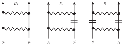
Figure 1: On-shell in-medium loop organized in the number of medium-insertions (=). The middle diagram has a reflected partner. The external momenta $\vec{p}_{1}$ and $\vec{p}_{2}$ are unconstrained.

The basic quantity in order to achieve the resummation of ladder diagrams to all orders in ref.[2] has been the complex-valued in-medium loop. Therefore, we calculate first the modifications of the in-medium loop which arise from the introduction of the test-particle with momentum $\vec{p}$. It is convenient to work with the half-sum $\vec{P}=(\vec{p}_{1}+\vec{p}_{2})/2$ and half-difference $\vec{q}=(\vec{p}_{1}-\vec{p}_{2})/2$ of two external momenta $\vec{p}_{1}$ and $\vec{p}_{2}$. In contrast to the calculation of the interaction energy per particle $\bar{E}(k_{f})$ in ref.[2], the external momenta $\vec{p}_{1}$ and $\vec{p}_{2}$ are now not constrained to lie inside a Fermi sphere of radius $k_{f}$. The real part of the on-shell in-medium loop comes from the (middle) diagram in Fig. 1 with one medium-insertion and after the substitution specified in eq.(2) it reads:

$${\rm Re}\,B_{1}=-4\pi a\int\!\!{d^{3}l\over(2\pi)^{3}}\,{1\over\vec{l}^{\,2}-\vec{q}^{\,2}}\Big{\{}N_{\eta}(\vec{P}+\vec{l},\vec{p}\,)+N_{\eta}(\vec{P}-\vec{l},\vec{p}\,)\Big{\}}\,.$$ (4)

The contribution linear in $\eta$ is simply twice the same energy denominator and after averaging over the directions of $\vec{p}$ one finds:

$${\rm Re}\,\bar{B}_{1}=-{ak_{f}\over\pi}\Big{\{}R(s,\kappa)+\tilde{\eta}\,\widehat{R}(s,\kappa,x)\Big{\}}\,,$$ (5)

with the dimensionless infinitesimal parameter $\tilde{\eta}=\eta\,\pi^{2}/k_{f}^{3}$ and the logarithmic functions:

$$R(s,\kappa)=2+{1\over 2s}[1-(s+\kappa)^{2}]\ln{1+s+\kappa\over|1-s-\kappa|}+{1\over 2s}[1-(s-\kappa)^{2}]\ln{|1+s-\kappa|\over|1-s+\kappa|}\,,$$ (6)

$$\widehat{R}(s,\kappa,x)={1\over sx}\ln{|(s+x)^{2}-\kappa^{2}|\over|(s-x)^{2}-\kappa^{2}|}\,,\qquad\qquad\widehat{R}(s,\kappa,0)={4\over s^{2}-\kappa^{2}}\,,$$ (7)

written in terms of the dimensionless variables $s=P/k_{f}$, $\kappa=q/k_{f}$ and $x=p/k_{f}$. Actually, the function $R(s,\kappa)$ will be needed later only in regions where $1+s-\kappa$ and $1-s+\kappa$ are both positive. Therefore, one could drop the absolute magnitudes in the argument of the second logarithm in eq.(6). An interesting relation between these functions is: $\int_{0}^{1}dx\,x^{2}\widehat{R}(s,\kappa,x)=R(s,\kappa)$.

Next, we consider the imaginary part of the on-shell in-medium loop. It is generated by all three diagrams in Fig. 1 and after inclusion of the perturbation by the test-particle it reads:

$${\rm Im}(B_{0}\!+\!B_{1}\!+\!B_{2}) = 4\pi^{2}a\int\!\!{d^{3}l\over(2\pi)^{3}}\,\delta(\vec{l}^{\,2}-\vec{q}^{\,2})\bigg{\{}N_{\eta}(\vec{P}+\vec{l},\vec{p}\,)\,N_{\eta}(\vec{P}-\vec{l},\vec{p}\,)$$ (8)

$$+\Big{[}1-N_{\eta}(\vec{P}+\vec{l},\vec{p}\,)\Big{]}\Big{[}1-N_{\eta}(\vec{P}-\vec{l},\vec{p}\,)\Big{]}\bigg{\}}\,.$$

Averaging again over the directions of $\vec{p}$, one finds to linear order in $\eta$:

$${\rm Im}(B_{0}\!+\!\bar{B}_{1}\!+\!\bar{B}_{2})=ak_{f}\Big{\{}I(s,\kappa)+\tilde{\eta}\,\widehat{I}(s,\kappa,x)\Big{\}}\,,$$ (9)

with the piecewise defined function:

$$I(s,\kappa)={1\over 2s}\,{\rm min}\Big{(}2s\kappa,|s^{2}+\kappa^{2}-1|\Big{)}\,.$$ (10)

In order to arrive at this compact form one has consider separately the pertinent arrangement of three shifted spheres in the case $0<s<1$, where changes of $I(s,\kappa)$ occur at $\kappa=1-s,\sqrt{1-s^{2}},\\ 1+s$, and in the case $s>1$, where changes of $I(s,\kappa)$ occur at $\kappa=s-1,s+1$. The correction term linear in $\tilde{\eta}$ is determined by the function:

$$\widehat{I}(s,\kappa,x)={1\over sx}\,\theta(s+\kappa-x)\,\theta(x-|s-\kappa|)\,{\rm sign}(1+x^{2}-2(s^{2}+\kappa^{2}))\,,$$ (11)

$$\widehat{I}(s,\kappa,0)={2\over s}\,\delta(s-\kappa)\,{\rm sign}(1-2s)\,.$$ (12)

The contribution of the diagram with two medium-insertion (i.e. the term in eq.(8) with two $N_{\eta}$-factors) is purely imaginary and after angular averaging it reads:

$$\bar{B}_{2}=2iak_{f}\Big{\{}I_{*}(s,\kappa)+\tilde{\eta}\,\widehat{I}_{*}(s,\kappa,x)\Big{\}}\,,$$ (13)

with the function

$$I_{*}(s,\kappa)=I(s,\kappa)\,\theta(1-s^{2}-\kappa^{2})=\bigg{\{}\kappa\,\theta(1-s-\kappa)+{1\over 2s}(1-s^{2}-\kappa^{2})\,\theta(s+\kappa-1)\bigg{\}}\,\theta(1-s^{2}-\kappa^{2})\,,$$ (14)

equal to the restriction of $I(s,\kappa)$ to the quarter unit disc $s^{2}+\kappa^{2}<1$, and the function

$$\widehat{I}_{*}(s,\kappa,x)={1\over sx}\,\theta(s+\kappa-x)\,\theta(x-|s-\kappa|)\,\theta(1+x^{2}-2(s^{2}+\kappa^{2}))\,,$$ (15)

$$\widehat{I}_{*}(s,\kappa,0)={2\over s}\,\delta(s-\kappa)\,\theta(1-2s)\,,$$ (16)

equal to the restriction of $\widehat{I}(s,\kappa,x)$ to its domain of positive values. A relation worth mentioning is: $\int_{0}^{1}dx\,x^{2}\widehat{I}_{*}(s,\kappa,x)=2I_{*}(s,\kappa)$. For the sake of completeness we note that the vacuum term $B_{0}$ in dimensional regularization is simply: $B_{0}=iak_{f}\kappa$. The support of the function $\widehat{I}_{*}(s,\kappa,x)$ in the $s\kappa$-plane is shown by the grey area in Fig. 2. For $0<x<1$ this region is pieced together by a rectangle and a circular wedge. In the case $x>1$ only a circular wedge with radius $\sqrt{(1+x^{2})/2}>1$ remains and the overlap of this circular wedge with the quarter unit disc, $s^{2}+\kappa^{2}<1$, vanishes for $x\geq\sqrt{2}$.

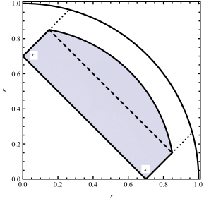
Figure 2: For $0<x<1$ the support of the function $\widehat{I}_{*}(s,\kappa,x)$ in the $s\kappa$-plane consists of a rectangle and a circular wedge. The rectangle has side-lengths $\sqrt{2}x$ and $(1-x)/\sqrt{2}$, the radius of the boundary circle is $\sqrt{(1+x^{2})/2}$. For $x>1$ this support consists only of a circular wedge.

2.2 Construction of the complex-valued single-particle potential

Having available the real and imaginary part of the (on-shell) in-medium loop with corrections linear in $\tilde{\eta}$, the complex single-particle potential $U(p,k_{f})+i\,W(p,k_{f})$ arising from ladder diagrams can be constructed in a one-step process from the expression for the resummed interaction density derived in ref.[2]:

$$V(\tilde{\eta})=-{4\pi a\over M}\sum_{n=1}^{\infty}\sum_{j=0}^{n-1}(B_{0}\!+\!\bar{B}_{1})^{n-1-j}\bar{B}_{2}^{\,j}{n\!-\!1\choose j}{1\over j\!+\!1}={4\pi a\over M\bar{B}_{2}}\,\ln{1-B_{0}-\bar{B}_{1}-\bar{B}_{2}\over 1-B_{0}-\bar{B}_{1}}\,.$$ (17)

The associated energy density is: ${\cal E}=(2\pi)^{-6}\int d^{3}p_{1}\int d^{3}p_{2}\,V(\tilde{\eta})N_{\eta}(\vec{p}_{1},\vec{p}\,)N_{\eta}(\vec{p}_{2},\vec{p}\,)$. There are two contributions to $U(p,k_{f})+i\,W(p,k_{f})$ of different kinematical origin. The “external” contribution comes from the last two momentum-space integrations that are introduced by the closing of open ladder diagrams. The interesting term linear in $\eta$ leads to an integral over $\theta(k_{f}-|\vec{p}_{1}|)\,\delta^{3}(\vec{p}_{2}-\vec{p}\,)$ times the resummed interaction density $V(\tilde{\eta})$ evaluated at $\tilde{\eta}=0$. The pertinent integral over a radius and a directional cosine can be transformed into the variables $(s,\kappa)$ and in the course of this transformation the function $s^{2}\kappa\,\widehat{I}_{*}(s,\kappa,x)$ arises as the appropriate weighting function. The “internal” contribution is an integral over $\theta(k_{f}-|\vec{p}_{1}|)\,\theta(k_{f}-|\vec{p}_{2}|)$ (i.e. the product of two Fermi spheres) where the integrand is equal to the first-order expansion coefficient in $\tilde{\eta}$ of the resummed interaction density $V(\tilde{\eta})$. The weighting function for this integral is $s^{2}\kappa\,I_{*}(s,\kappa)$ (see eq.(15) in ref.[2]). Since the external and internal contribution carry the same prefactor $2k_{f}^{3}/\pi^{2}$, the complex single-particle potential is completely determined by the quantity: $\widehat{I}_{*}\,V(0)+I_{*}\,V^{\prime}(0)$. It has to be analyzed and decomposed into real and imaginary part on the different integration domains in the $s\kappa$-plane (i.e. the supports of $I_{*}(s,\kappa)$ and $\widehat{I}_{*}(s,\kappa,x)$) separately for $0<x<1$ and $x>1$.

Let us consider first the on-shell single-particle potential for momenta $p<k_{f}$ inside the Fermi sphere. After the cancellation of a term proportional to arctangent-function one arrives at the following concise double-integral representation for the real single-particle potential as derived from the resummed particle-particle and hole-hole ladder diagrams:

$$U(p,k_{f}) = {8ak_{f}^{3}\over M}\int\limits_{0}^{1}\!ds\,s^{2}\!\!\int\limits_{0}^{\sqrt{1-s^{2}}}\!\!d\kappa\,\kappa\,\Bigg{\{}{ak_{f}\widehat{R}(s,\kappa,x)I(s,\kappa)-\widehat{I}_{*}(s,\kappa,x)[\pi+ak_{f}R(s,\kappa)]\over[\pi+ak_{f}R(s,\kappa)]^{2}+[ak_{f}\pi\,I(s,\kappa)]^{2}}$$ (18)

$$\qquad\qquad\qquad\qquad\qquad-{1\over ak_{f}}\widehat{R}(s,\kappa,x)\,\delta\bigg{(}{\pi\over ak_{f}}+R(s,\kappa)\bigg{)}\Bigg{\}}\,.$$

The occurrence of the last $\delta$-function term in eq.(18) is very subtle. A careful inspection of the mathematical expressions reveals that it is produced by differentiating the discontinuity of the arctangent-function at infinity. The arctangent-function makes a jump by $-\pi$, when the denominator $\pi/ak_{f}+R(s,\kappa)+\tilde{\eta}\,\widehat{R}(s,\kappa,x)$ of its argument passes through zero from positive to negative values. The $\delta$-function term  is treated numerically by first searching the line $\kappa(s)$ on which $R(s,\kappa(s))=-\pi/ak_{f}$ and then integrating over the appropriate $s$-interval with the weighting function $|\partial R(s,\kappa)/\partial\kappa|^{-1}$. The line of zeros of the function $R(s,\kappa)$ inside the unit quarter disc is shown by the (lower) dashed-dotted line in Fig. 3. This curve starts at $s_{0}=0$, $\kappa_{0}=0.83356$ and ends at $s_{1}=0.55243$, $\kappa_{1}=0.83356=\kappa_{0}$. Alternatively, the $\delta$-function term can be treated in a regularized form such as: $\pi\,\delta(X)=\lim_{\epsilon\to 0^{+}}\epsilon/(X^{2}+\epsilon^{2})$. One finds that finite $\epsilon\simeq 10^{-3}$ give sufficiently accurate numerical results.

Figure 3: The function $R(s,\kappa)$ defined in eq.(6) is zero along the (lower) dashed-dotted line. The function $F(s,\kappa)$ defined in eq.(40) is zero along the (upper) dashed line.

The imaginary single-particle potential for momenta $p<k_{f}$ inside the Fermi sphere is given by a simpler expression:

$$W(p,k_{f})={8\pi a^{2}k_{f}^{4}\over M}\int\limits_{0}^{1}\!ds\,s^{2}\!\!\int\limits_{0}^{\sqrt{1-s^{2}}}\!\!d\kappa\,\kappa\,{[\widehat{I}_{*}(s,\kappa,x)-\widehat{I}(s,\kappa,x)]\,I(s,\kappa)\over[\pi+ak_{f}R(s,\kappa)]^{2}+[ak_{f}\pi\,I(s,\kappa)]^{2}}\,.$$ (19)

Note that this integral receives contributions only from circular ring region indicated in Fig. 2 by the dotted lines where the function $\widehat{I}(s,\kappa,x)$ is negative and $\widehat{I}_{*}(s,\kappa,x)$ vanishes. Consequently, $W(p,k_{f})>0$ is positive for all $p<k_{f}$ as required for the stability of hole states in the Fermi sea. The important constraint $W(k_{f},k_{f})=0$ (Luttinger’s theorem [12]) is also obvious from the representation in eq.(19), since at $x=1$ the integration region in the $s\kappa$-plane vanishes identically.

2.3 Continuation into the region outside the Fermi sphere

Next, we consider the complex single-particle potential for momenta $p>k_{f}$ outside the Fermi sphere. The new element here is that the pertinent integration region in the $s\kappa$-plane is now larger than the quarter unit disc. The contribution to the real single-particle potential $U(p,k_{f})$ from the region $s^{2}+\kappa^{2}<1$ is of the same form as described in subsection 2.2. The corresponding integral will include the weighting function $\theta(1-s^{2}-\kappa^{2})$. The “external” contribution from the region $s^{2}+\kappa^{2}>1$ requires to take the limit $\tilde{\eta}\to 0$ because of the factor $1/\tilde{\eta}$ which comes from $1/\bar{B}_{2}$ in $V(\tilde{\eta})$, when $I_{*}(s,\kappa)=0$. In effect the “external” piece continues the term proportional to $\widehat{I}_{*}(s,\kappa,x)$ that is already present in the “internal” piece into the region $s^{2}+\kappa^{2}>1$. The complete expression for the real single-particle potential $U(p,k_{f})$ outside the Fermi sphere $p>k_{f}$ reads:

$$U(p,k_{f}) \!\!\!\!=\!\!\!\! {8ak_{f}^{3}\over M}\int\limits_{0}^{(x+1)/2}\!ds\,s^{2}\!\!\int\limits_{0}^{(x+1)/2}\!\!d\kappa\,\kappa\,\Bigg{\{}{ak_{f}\widehat{R}(s,\kappa,x)I_{*}(s,\kappa)-\widehat{I}_{*}(s,\kappa,x)[\pi+ak_{f}R(s,\kappa)]\over[\pi+ak_{f}R(s,\kappa)]^{2}+[ak_{f}\pi\,I(s,\kappa)]^{2}}$$ (20)

$$\qquad\qquad\qquad\qquad\qquad\qquad-\,{\theta(1-s^{2}-\kappa^{2})\over ak_{f}}\widehat{R}(s,\kappa,x)\,\delta\bigg{(}{\pi\over ak_{f}}+R(s,\kappa)\bigg{)}\Bigg{\}}\,.$$

Note that the square of side-length $(x+1)/2>1$ is large enough to cover the relevant integration regions (the quarter unit disc and the circular wedge of radius $\sqrt{(1+x^{2})/2}>1$) in the $s\kappa$-plane.

The calculation of the “external” contribution from the region $s^{2}+\kappa^{2}>1$ through taking the limit $\tilde{\eta}\to 0$ gives rise to a complex-valued single-particle potential, whose imaginary part reads:

$$W(p,k_{f})=-{8\pi a^{2}k_{f}^{4}\over M}\int\limits_{0}^{(x+1)/2}\!ds\,s^{2}\!\!\int\limits_{0}^{(x+1)/2}\!\!d\kappa\,\kappa\,{\widehat{I}_{*}(s,\kappa,x)I(s,\kappa)\,\theta(s^{2}+\kappa^{2}-1)\over[\pi+ak_{f}R(s,\kappa)]^{2}+[ak_{f}\pi\,I(s,\kappa)]^{2}}\,.$$ (21)

Note that for $x>\sqrt{2}$ the condition $s^{2}+\kappa^{2}>1$ can be dropped since then the support of the weighting function $\widehat{I}_{*}(s,\kappa,x)$ (a circular wedge) lies completely in the outer region. The integrand in eq.(21) is obviously positive and therefore $W(p,k_{f})<0$ is negative for all $p>k_{f}$ as required for the stability of particle states outside the Fermi sphere.

2.4 Hugenholtz-Van-Hove theorem

An important constraint on the single-particle potential is given by the Hugenholtz-Van-Hove theorem [13]. It states that the total single-particle energy $U(k_{f},k_{f})+k_{f}^{2}/2M$ at the Fermi surface $p=k_{f}$ is equal to the chemical potential. By a general thermodynamical relation the chemical potential is equal to the derivative of the energy density $\rho\,(\bar{E}(k_{f})+3k_{f}^{2}/10M)$ with respect to the particle density $\rho=k_{f}^{3}/3\pi^{2}$. We prove now that the Hugenholtz-van-Hove theorem is satisfied in the present non-perturbative calculation. The starting point is the resummed (interaction) energy per particle $\bar{E}(k_{f})$ as given by eq.(14) in ref.[2]. First, one calculates the derivative with the respect to $k_{f}$ in that given double-integral representation. Then, one remembers that the interaction energy density was originally an integral over the product of two Fermi spheres, $\theta(k_{f}-|\vec{p}_{1}|)\,\theta(k_{f}-|\vec{p}_{2}|)$, and differentiates separately the integration boundaries and the integrand with respect to $k_{f}$. The described procedure translates into the following sequence of equations:

$$\bar{E}(k_{f})+{k_{f}\over 3}{\partial\bar{E}(k_{f})\over\partial k_{f}}=-{8k_{f}^{2}\over\pi M}\int\limits_{0}^{1}\!ds\,s^{2}\!\!\int\limits_{0}^{\sqrt{1-s^{2}}}\!\!d\kappa\,\Bigg{\{}5\arctan{ak_{f}I(s,\kappa)\over 1+ak_{f}\pi^{-1}R(s,\kappa)}$$

$$+{ak_{f}I(s,\kappa)\over[1+ak_{f}\pi^{-1}R(s,\kappa)]^{2}+[ak_{f}I(s,\kappa)]^{2}}-{\pi^{2}\over ak_{f}}\,\delta\bigg{(}{\pi\over ak_{f}}+R(s,\kappa)\bigg{)}\Bigg{\}}$$

$$={8ak_{f}^{3}\over M}\int\limits_{0}^{1}\!ds\,s^{2}\!\!\int\limits_{0}^{\sqrt{1-s^{2}}}\!\!d\kappa\,\kappa\,\Bigg{\{}{ak_{f}\widehat{R}(s,\kappa,1)I(s,\kappa)-\widehat{I}_{*}(s,\kappa,1)[\pi+ak_{f}R(s,\kappa)]\over[\pi+ak_{f}R(s,\kappa)]^{2}+[ak_{f}\pi\,I(s,\kappa)]^{2}}$$

$$\hskip 128.0374pt-{1\over ak_{f}}\widehat{R}(s,\kappa,1)\,\delta\bigg{(}{\pi\over ak_{f}}+R(s,\kappa)\bigg{)}\Bigg{\}}=U(k_{f},k_{f})\,,$$ (22)

where the equality between the initial and final term is precisely the statement of the Hugenholtz-Van-Hove theorem [13]. In order to establish the agreement with $U(k_{f},k_{f})$ the following identities have been instrumental:

$${\partial\over\partial k_{f}}\Big{[}k_{f}R(P/k_{f},q/k_{f})\Big{]}={1\over s}\ln{(s+1)^{2}-\kappa^{2}\over|(s-1)^{2}-\kappa^{2}|}=\widehat{R}(s,\kappa,1)\,,$$ (23)

$${\partial\over\partial k_{f}}\Big{[}k_{f}I(P/k_{f},q/k_{f})\Big{]}={1\over s}\,\theta(s+\kappa-1)=\widehat{I}_{*}(s,\kappa,1)\,,$$ (24)

where the derivative with respect to $k_{f}$ is taken at fixed $P$ and $q$, and the constraint $s^{2}+\kappa^{2}<1$ holds here. Note that the arctangent-function in eq.(22) refers to the usual branch with odd parity, $\arctan(-X)=-\arctan X$, and values in the interval $[-\pi/2,\pi/2]$. Other branches of the arctangent-function are excluded by the weak coupling limit $a\to 0$, which has to give zero independently of the sign of the scattering length $a$. The $\delta$-function terms in both double-integral expressions in eq.(22) are crucial for the actual numerical validity of the Hugenholtz-Van-Hove theorem. We have examined this over a wide range of positive and negative values of the dimensionless coupling strength $ak_{f}$. In fact the violation of the Hugenholtz-Van-Hove theorem without the $\delta$-function terms has given the hint that there is this subtlety in differentiating the arctangent-function (as explained in the subsection 2.2).

The slope of the (on-shell) single-particle potential at the Fermi surface $p=k_{f}$ determines the density-dependent effective mass $M^{*}(k_{f})$ of the (stable) quasi-particle excitations at the Fermi surface. The corresponding relation for the effective mass $M^{*}(k_{f})$ reads:

$${1\over M^{*}(k_{f})}={1\over M}+{1\over k_{f}}\,{\partial U(p,k_{f})\over\partial p}\bigg{|}_{p=k_{f}}\,,$$ (25)

with $M$ the free fermion mass.

2.5 Perturbative expansion

Given the closed-form expressions for the complex single-particle potential $U(p,k_{f})+i\,W(p,k_{f})$ in eqs.(18-21), one can expand them in powers of the scattering length $a$. It is convenient to scale out the free Fermi energy $k_{f}^{2}/2M$ and to use a dimensionless expansion parameter, such that the perturbative series reads:

$$U(p,k_{f})+i\,W(p,k_{f})={k_{f}^{2}\over 2M}\sum_{n=1}^{\infty}(-ak_{f})^{n}\Big{[}\Phi_{n}(x)+i\,\Omega_{n}(x)\Big{]}\,.$$ (26)

Here, the dimensionless functions $\Phi_{n}(x)$ and $\Omega_{n}(x)$ describe the momentum dependence of the real and imaginary part at $n$-th order. Note that the $\delta$-function term in eqs.(18,20) proportional to $\delta(\pi+ak_{f}R(s,\kappa))$ does not contribute at any order in the expansion in powers of $-ak_{f}$. In this sense it represents a truly non-perturbative term. The first order contribution to the perturbative expansion in eq.(26) is the trivial Hartree-Fock mean field result:

$$\Phi_{1}(x)={4\over 3\pi}\,,\qquad\Omega_{1}(x)=0\,,$$ (27)

and the second order contribution to the complex single-particle potential is known from the classical work by Galitskii [14]. The corresponding function $\Phi_{2}(x)$ has for $0<x<1$ the form:

$$\Phi_{2}(x)={4\over 15\pi^{2}}\Bigg{\{}11-2x^{4}\ln{1-x^{2}\over x^{2}}+{10\over x}(1-x^{2})\ln{1+x\over 1-x}-{2\over x}(2-x^{2})^{5/2}\ln{1+x\sqrt{2-x^{2}}\over 1-x^{2}}\Bigg{\}}\,,$$ (28)

and it gets continued into the region $x>1$ by the expression:

$$\Phi_{2}(x) = {4\over 15\pi^{2}}\Bigg{\{}11-2x^{4}\ln{x^{2}-1\over x^{2}}+{10\over x}(1-x^{2})\ln{x+1\over x-1}-{2\over x}\bigg{[}\theta(\sqrt{2}-x)\,$$ (29)

$$\times(2-x^{2})^{5/2}\ln{1+x\sqrt{2-x^{2}}\over x^{2}-1}+\theta(x-\sqrt{2})\,(x^{2}-2)^{5/2}\arcsin{1\over x^{2}-1}\bigg{]}\Bigg{\}}\,.$$

The function $\Omega_{2}(x)$ describing the leading contribution to the imaginary potential has the form:

$$\Omega_{2}(x)={\theta(1-x)\over 2\pi}\,(1-x^{2})^{2}+{2\,\theta(x-1)\over 15\pi x}\,\Big{\{}7-5x^{2}-2(2-x^{2})^{5/2}\,\theta(\sqrt{2}-x)\Big{\}}\,.$$ (30)

The elaborate function $\Phi_{2}(x)$ has the boundary values $\Phi_{2}(0)=4/\pi^{2}$, $\Phi_{2}(1)=4(11-2\ln 2)/15\pi^{2}$ and the slope $\Phi_{2}^{\prime}(1)=16(1-7\ln 2)/15\pi^{2}$ at $x=1$. A good approximation of $\Phi_{2}(x)$ for $x>5/3$ is provided by the asymptotic expansion: $\pi^{2}\Phi_{2}(x)=(16/9x^{2})+(22/45x^{4})+(32/105x^{6})+{\cal O}(x^{-8})$.

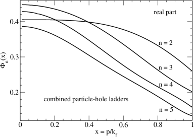
Figure 4: Momentum dependence of perturbative contributions to the real single-particle potential inside the Fermi sphere.

The agreement at first order follows from the value of the integral: $\int\!ds\,s^{2}\!\int\!d\kappa\,\kappa\,\widehat{I}_{*}(s,\kappa,x)=1/12$, which applies both for $0<x<1$ and $x>1$. In the same way, the double-integral representations of $\Phi_{2}(x)$ and $\Omega_{2}(x)$ which one obtains by expanding eqs.(18-21) to second order in $ak_{f}$ are in perfect numerical agreement (at the 6-digit level) with the analytical expressions written in eqs.(28-30), both for $0<x<1$ and $x>1$. This agreement provides a very important check on the formalism introduced in subsection 2.1 in order to construct non-perturbatively the complex single-particle potential $U(p,k_{f})+i\,W(p,k_{f})$. While results for the interaction energy per particle $\bar{E}(k_{f})$ are available up to fourth order [3, 4], the on-shell single-particle potential $U(p,k_{f})+i\,W(p,k_{f})$ has so far not been computed beyond second order. At this point the present calculation provides a multitude of new results. One should note that at third and higher order in $ak_{f}$ there exist also other classes of diagrams, such as the particle-hole ring diagrams [5]. The corresponding real single-particle potential $U(p,k_{f})^{n-\rm ring}$ is studied in section 4.

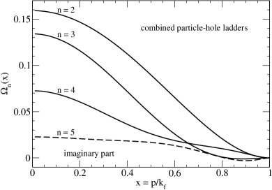
Figure 5: Momentum dependence of perturbative contributions to the imaginary single-particle potential inside the Fermi sphere.

The $x$-dependence of the functions $\Phi_{n}(x)$ and $\Omega_{n}(x)$ for $n=2,3,4,5$ in the region $0<x<1$ is shown in Figs. 4,5. One observes a decrease of the $n$-th order potential-functions as one moves from $x=0$ (bottom of the Fermi sea) to $x=1$ (at the Fermi surface). There is also a tendency that higher-order functions get smaller in magnitude. Precise numerical values of the boundary values $\Phi_{n}(0)$, $\Omega_{n}(0)$ and $\Phi_{n}(1)$ are listed in Table 1 up to order $n=8$. The values $\Phi_{n}(0)$ and $\Omega_{n}(0)$ have been computed by using the explicit expressions for $\widehat{R}(s,\kappa,0)$, $\widehat{I}(s,\kappa,0)$ and $\widehat{I}_{*}(s,\kappa,0)$ written in eqs.(7,12,16). The analytical value $\Omega_{3}(0)=16[2\sqrt{2}\ln(1+\sqrt{2})-3\ln 2]/5\pi^{2}$ associated to the imaginary single-particle potential at third order is obtained as a byproduct of this calculation. The right boundary values $\Phi_{n}(1)$ are furthermore determined by the Hugenholtz-Van-Hove theorem. One has the relation $\Phi_{n}(1)=(2/\pi)^{n}(n+5)\,c_{n}/9$, where the coefficients $c_{n}$ have been defined through the $k_{f}$-expansion of $\bar{E}(k_{f})$ in eq.(19) of ref.[2]. Inserting the numerical values of $c_{n}$ listed in eq.(20) of ref.[2] one finds perfect agreement with the values of $\Phi_{n}(1)$ calculated directly via the perturbative expansion of $U(p,k_{f})$. This demonstrates that the Hugenholtz-Van-Hove theorem is fulfilled order by order without the $\delta$-function term in eq.(18).

$n$	1	2	3	4	5	6	7	8
$\Phi_{n}(0)$	0.42441	0.40528	0.44788	0.42857	0.38638	0.33254	0.28779	0.25073
$\Omega_{n}(0)$		0.15915	0.13406	0.07256	0.02273	–0.00496	–0.01414	–0.01237
$\Phi_{n}(1)$	0.42441	0.25975	0.20153	0.15744	0.13314	0.11153	0.09959	0.08573
$\Psi_{n}(0)$	0.42441	0.40528	0.35745	0.29486	0.23203	0.17676	0.13168	0.09658
$\Xi_{n}(0)$		0.15915	0.16809	0.13425	0.09601	0.06479	0.04222	0.02689
$\Psi_{n}(1)$	0.42441	0.25975	0.17083	0.11493	0.07872	0.05444	0.03797	0.02663

Table 1: Boundary values of the functions $\Phi_{n}(x)$, $\Omega_{n}(x)$, $\Psi_{n}(x)$ and $\Xi_{n}(x)$ describing the momentum dependence of perturbative contributions to the complex single-particle potential. The values $\Phi_{n}(1)$ and $\Psi_{n}(1)$ are fixed by the Hugenholtz-Van-Hove theorem.

The continuation of the potential-functions $\Phi_{n}(x)$ and $\Omega_{n}(x)$ for $n=2,3,4,5$ into the region $1<x<2$ outside the Fermi sphere is shown in Figs. 6,7. The behavior with increasing $x$ is nonuniform and alternates for different orders including even changes of the sign. Note that a small positive contribution to the imaginary single-particle potential $W(p,k_{f})$ for $p>k_{f}$ at higher orders in the perturbative expansion is compatible with the stability (i.e. damping) of quasi-particle excitations.

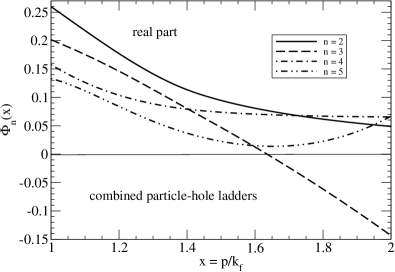
Figure 6: Momentum dependence of perturbative contributions to the real single-particle potential outside the Fermi sphere.

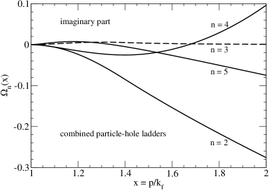
Figure 7: Momentum dependence of perturbative contributions to the imaginary single-particle potential outside the Fermi sphere.

2.6 Strong coupling limit

The limit $a\to\infty$ is of special interest since in this limit the strongly interacting many-fermion system becomes scale invariant. Returning to the expressions for the resummed single-particle potential $U(p,k_{f})+i\,W(p,k_{f})$ in eqs.(18-21), one sees that the limit $a\to-\infty$ (in the repulsive regime) can be performed straightforwardly. The resulting real and imaginary part read for $p<k_{f}$:

$$U(p,k_{f})^{(\infty)} \!\!\!=\!\!\! {8k_{f}^{2}\over M}\int\limits_{0}^{1}\!ds\,s^{2}\!\!\int\limits_{0}^{\sqrt{1-s^{2}}}\!\!d\kappa\,\kappa\,\Bigg{\{}{\widehat{R}(s,\kappa,x)I(s,\kappa)-\widehat{I}_{*}(s,\kappa,x)R(s,\kappa)\over R(s,\kappa)^{2}+\pi^{2}I(s,\kappa)^{2}}-\widehat{R}(s,\kappa,x)\,\delta(R(s,\kappa))\Bigg{\}}$$ (31)

$$\!\!\!=\!\!\! {k_{f}^{2}\over 2M}\,\Phi_{\rm uni}(x)\,,$$

$$W(p,k_{f})^{(\infty)}={8\pi k_{f}^{2}\over M}\int\limits_{0}^{1}\!ds\,s^{2}\!\!\int\limits_{0}^{\sqrt{1-s^{2}}}\!\!d\kappa\,\kappa\,{[\widehat{I}_{*}(s,\kappa,x)-\widehat{I}(s,\kappa,x)]\,I(s,\kappa)\over R(s,\kappa)^{2}+\pi^{2}I(s,\kappa)^{2}}={k_{f}^{2}\over 2M}\,\Omega_{\rm uni}(x)\,,$$ (32)

and the modifications of these formulas for $p>k_{f}$ are obvious from eqs.(20,21). The dimensionless functions $\Phi_{\rm uni}(x)$ and $\Omega_{\rm uni}(x)$ describe the dependence on the rescaled momentum variable $x=p/k_{f}$. The calculated boundary values are:

$$\Phi_{\rm uni}(0)=-0.214\,,\qquad\Phi_{\rm uni}(1)=\xi_{n}-1=-0.493\,,\qquad\Omega_{\rm uni}(0)=0.780\,,$$ (33)

with $\xi_{n}=0.507$ the normal Bertsch parameter obtained in ref.[2]. Note that the value $\Phi_{\rm uni}(1)=\xi_{n}-1$ is fixed by the Hugenholtz-Van-Hove theorem and interestingly it is almost entirely determined by the contribution of the $\delta$-function term in eq.(31): $\Phi_{\rm uni}(1)=-0.031-0.462$. Given the two negative boundary values in eq.(33) one would expect a monotonically decreasing function $\Phi_{\rm uni}(x)$. However, the numerical evaluation of the full expression for $\Phi_{\rm uni}(x)$ in eq.(31) leads to a completely different result, which is shown by the full line in Fig. 8. The function $\Phi_{\rm uni}(x)$ rises steeply into the positive domain, it develops a peak of height $0.98$ at $x\simeq 0.3$, and then drops back to negative values. The negative slope of $\Phi_{\rm uni}(x)$ at $x=1$ translates into an enhanced effective mass of $M^{*}/M=[1+\Phi^{\prime}_{\rm uni}(1)/2]^{-1}\simeq 2.1$. The average value of $\Phi_{\rm uni}(x)$ taken over the interior of the Fermi sphere is: $3\int_{0}^{1}dx\,x^{2}\Phi_{\rm uni}(x)=-48\int ds\,s^{2}\int d\kappa\,\kappa\,I_{*}R/(R^{2}+\pi^{2}I^{2})=-0.224$. This is rather close to the value $\Phi_{\rm uni}(0)=-0.214$ at the bottom of the Fermi sea. Furthermore, one observes that the function $\Omega_{\rm uni}(x)$ associated to the imaginary single-particle potential $W(p,k_{f})^{(\infty)}$ follows the up- and downward motion of $\Phi_{\rm uni}(x)$. This feature implies that the peculiar unbound hole excitations with momenta $0.2k_{f}<p<0.5k_{f}$ are at the same time also very short-lived.

The strong momentum dependence of the potential $U(p,k_{f})^{(\infty)}$ indicates an instability against a (topological) phase transition to a state with separation in momentum space [8, 15, 16]. Namely, if one adds the kinetic energy $p^{2}/2M$ to the potential $U(p,k_{f})^{(\infty)}$, one finds a momentum region where the full single-particle energy lies above the (interacting) Fermi energy $\xi_{n}k_{f}^{2}/2M$. In Fig. 13 this corresponds to the interval $0.272<x<0.415$, inside which $\Phi_{\rm uni}(x)>\xi_{n}-x^{2}$ holds. But states lying above the Fermi energy will not be occupied, so one gets an empty shell (or bubble) in the Fermi sea, which reduces the density by about $5\%$ to $0.95\,k_{f}^{3}/3\pi^{2}$. Such a bubble formation in neutron matter (which could have important consequences for neutron star cooling) has been discussed in ref.[16] in connection with the possibility of neutral pion condensation. According to the present calculation the low-energy neutron-neutron interaction, as represented by the large $nn$-scattering length $a_{nn}=19\,$fm, could likewise induce the instability to this (topological) phase transition. When analyzing the potential $U(p,k_{f})$ in eq.(18) at finite coupling strength $ak_{f}$, one finds in a numerical study that the instability occurs for $ak_{f}>5.5$ and $ak_{f}<-3.0$.

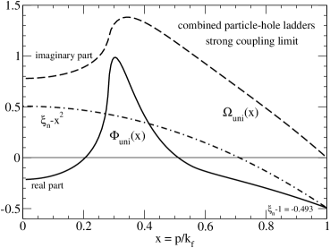
Figure 8: Momentum dependence of the single-particle potential inside the Fermi sphere in the limit $a\to\infty$.

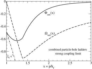
Figure 9: Momentum dependence of the single-particle potential outside the Fermi sphere in the limit $a\to\infty$.

The continuation of the functions $\Phi_{\rm uni}(x)$ and $\Omega_{\rm uni}(x)$ into the region $x>1$ outside the Fermi surface is shown in Fig. 9. One observes that $\Phi_{\rm uni}(x)$ reaches its minimum value of $-0.629$ at $x\simeq 1.25$ and from there on it decreases rapidly in magnitude with increasing $x=p/k_{f}$. The other function $\Omega_{\rm uni}(x)$ drops linearly from zero at $x=1$ to its minimum value of $-0.909$ at $x\simeq 1.4$ and from there on it decreases slowly in magnitude with increasing $x$. This means that particle excitations with relatively high momentum get weakly attracted by fermionic medium and are at the same time very short-lived. The asymptotic behavior of the function $\Omega_{\rm uni}(x)$ for large $x$ is:

$$\Omega_{\rm uni}(x)=-{8\over 3\pi x}\bigg{(}1+{8\over 5x^{2}}+{4\over 3x^{4}}-{1\over x^{6}}+\dots\bigg{)}\,,$$ (34)

with coefficients determined in an extensive numerical study. The reason for such a simple asymptotic form is the integration region in eq.(21) which becomes for large $x$ a very thin circular wedge spanned between the points $((x-1)/2,(x+1)/2)$ and $((x+1)/2,(x-1)/2)$ in the $s\kappa$-plane. In this situation simplifying approximations will hold for the functions $R(s,\kappa)$ and $I(s,\kappa)$ in the integrand.

Another special feature visible from Figs. 8,9 is that the imaginary part $\Omega_{\rm uni}(x)$ vanishes linearly at the Fermi surface $x=1$, with the same slope $\Omega_{\rm uni}^{\prime}(1)=-4\pi(s_{1}\kappa_{1})^{2}=-2.6647$ from both sides. Indeed, when evaluating numerically $W(p,k_{f})$ in eqs.(19,21) at small coupling strength $|ak_{f}|<1/2$ one finds the quadratic behavior $\pm(1-x)^{2}$ according to Luttinger’s theorem [12]. However, for large coupling this degenerates to a linear behavior. Let us point to the origin of this unconventional property. The numerator in the representations of $W(p,k_{f})$ in eqs.(19,21) alone would lead to the quadratic behavior $\pm(1-x)^{2}$, but there is also the denominator (due to resummation) which introduces a singular region into the double-integral. In principle the linear behavior $1-x$, which is caused by the vanishing of $R(s,\kappa)+\pi/ak_{f}$ on the unit-circle $s^{2}+\kappa^{2}=1$, is present for all coupling strengths $ak_{f}>0$ and $ak_{f}<-\pi/2$. Using the dimensionless function $\Omega(x)=2Mk_{f}^{-2}\,W(p,k_{f})$, one finds in a careful analysis the following result for the (negative) slope at the Fermi surface $x=1$:

$$\Omega^{\prime}(1)=-{8\pi s_{1}^{2}(1-s_{1}^{2})\over 2+\pi(ak_{f})^{-1}s_{1}^{2}}\,,$$ (35)

where $0<s_{1}<1$ is the solution of the equation $R(s_{1},\sqrt{1-s_{1}^{2}})=-\pi/ak_{f}$. Interestingly, the largest negative slope $\Omega^{\prime}(1)\simeq-2\pi$ is not reached at infinite coupling, but for $ak_{f}\simeq-\pi/2$ (approached from below).

3 Particle-particle ladder diagrams only

In this section we perform the analogous construction of the complex single-particle potential $U(p,k_{f})+i\,W(p,k_{f})$ for the particle-particle ladder diagrams. This subclass of diagrams can be summed to all orders in the form of a geometrical series [5]. The momentum regions $p<k_{f}$ (inside the Fermi sphere) and $p>k_{f}$ (outside the Fermi surface) need to be considered separately.

The starting point is again the pertinent in-medium loop (also called particle-particle bubble function [5]). With inclusion of the test-particle with momentum $\vec{p}$ (see eq.(2)), the on-shell in-medium loop takes now the form:

$$B_{p}=4\pi a\int\!\!{d^{3}l\over(2\pi)^{3}}\,{1\over\vec{l}^{\,2}-\vec{q}^{\,2}-i\epsilon}\Big{[}1-N_{\eta}(\vec{P}+\vec{l},\vec{p}\,)\Big{]}\Big{[}1-N_{\eta}(\vec{P}-\vec{l},\vec{p}\,)\Big{]}\,,$$ (36)

where each factor $1-N_{\eta}(\dots)$ describes a particle phase-space. Averaging again over the directions of $\vec{p}$, one gets to linear order in the parameter $\tilde{\eta}=\eta\,\pi^{2}/k_{f}^{3}$:

$${\rm Re}\,\bar{B}_{p}=-{ak_{f}\over\pi}\Big{\{}F(s,\kappa)+\tilde{\eta}\,\widehat{F}(s,\kappa,x)\Big{\}}\,,$$ (37)

$${\rm Im}\,\bar{B}_{p}=ak_{f}\Big{\{}I(s,\kappa)-I_{*}(s,\kappa)+\tilde{\eta}\,\Big{[}\widehat{I}(s,\kappa,x)-\widehat{I}_{*}(s,\kappa,x)\Big{]}\Big{\}}\,,$$ (38)

with the functions $I(s,\kappa)-I_{*}(s,\kappa)$ and $\widehat{I}(s,\kappa,x)-\widehat{I}_{*}(s,\kappa,x)$ determined by the analytical expressions written in eqs.(10-16). The interaction density of the resummed particle-particle ladder diagrams is a geometrical series and it has the form:

$$V_{p}(\tilde{\eta})=-{4\pi a\over M}\sum_{n=1}^{\infty}\bar{B}_{p}^{\,n-1}={4\pi a\over M(\bar{B}_{p}-1)}\,.$$ (39)

3.1 Single-particle potential inside the Fermi sphere

For the single-particle potential inside the Fermi sphere the pertinent integration region in the $s\kappa$-plane is the quarter unit disc $s^{2}+\kappa^{2}<1$. Taking into account this constraint on the variables $(s,\kappa)$ the functions $F(s,\kappa)$ and $\widehat{F}(s,\kappa,x)$ introduced in eq.(37) are given by the expressions:

$$F(s,\kappa)=1+s-\kappa\ln{1+s+\kappa\over 1+s-\kappa}+{1\over 2s}(1-s^{2}-\kappa^{2})\ln{(1+s)^{2}-\kappa^{2}\over 1-s^{2}-\kappa^{2}}\,,$$ (40)

$$\widehat{F}(s,\kappa,x) = {1\over sx}\Bigg{\{}\theta(2s-1)\,\theta(2s-1-x)\ln{|(s+x)^{2}-\kappa^{2}|\over|(s-x)^{2}-\kappa^{2}|}$$ (41)

$$\qquad+\,\theta(x-|2s-1|)\ln{2|(s+x)^{2}-\kappa^{2}|\over|1+x^{2}-2(s^{2}+\kappa^{2})|}\Bigg{\}}\,,$$

$$\widehat{F}(s,\kappa,0)={4\,\theta(2s-1)\over s^{2}-\kappa^{2}}\,.$$ (42)

where $x$ lies in the interval $0<x<1$. Note that a factor $1-\theta(k_{f}-|2\vec{P}-\vec{p}\,|)$ is involved in the angular averaging procedure that generates the function $\widehat{F}(s,\kappa,x)$. This feature requires to study separately the cases $0<s<1/2$ and $1/2<s<1$. An interesting relation between these functions is: $\int_{0}^{1}dx\,x^{2}\widehat{F}(s,\kappa,x)=F(s,\kappa)-{\rm Re}\,F(-s,\kappa)$. It involves the difference of two terms, while the corresponding sum is given by: $F(s,\kappa)+{\rm Re}\,F(-s,\kappa)=R(s,\kappa)$.

Following the construction of the complex single-particle potential by means of the interaction density as described in section 2.2, one obtains from $V_{p}(\tilde{\eta})$ in eq.(39) the following double-integral representations for the real and imaginary part:

$$U(p,k_{f})={8ak_{f}^{3}\over M}\int\limits_{0}^{1}\!ds\,s^{2}\!\!\int\limits_{0}^{\sqrt{1-s^{2}}}\!\!d\kappa\,\kappa\,\Bigg{\{}{ak_{f}\widehat{F}(s,\kappa,x)I(s,\kappa)\over[\pi+ak_{f}F(s,\kappa)]^{2}}-{\widehat{I}_{*}(s,\kappa,x)\over\pi+ak_{f}F(s,\kappa)}\Bigg{\}}\,,$$ (43)

$$W(p,k_{f})={8\pi a^{2}k_{f}^{4}\over M}\int\limits_{0}^{1}\!ds\,s^{2}\!\!\int\limits_{0}^{\sqrt{1-s^{2}}}\!\!d\kappa\,\kappa\,{[\widehat{I}_{*}(s,\kappa,x)-\widehat{I}(s,\kappa,x)]I(s,\kappa)\over[\pi+ak_{f}F(s,\kappa)]^{2}}\,.$$ (44)

The denominator functions in eqs.(43,44) possess lines of zeros and therefore they have to be interpreted as (regularized) distributions: $X^{-\nu}={\rm Re}\lim_{\epsilon\to 0}(X+i\epsilon)^{-\nu}$ for $\nu=1,2$. The line of zeros of the function $F(s,\kappa)$ inside the unit quarter disc is shown be the (upper) dashed line in Fig. 3. This curve starts at $s_{0}=0$, $\kappa_{0}=0.83356$ and ends at $s_{1}=0.40865$, $\kappa_{1}=0.91269$.

In order to prove the validity of the Hugenholtz-Van-Hove theorem for the single-particle potential $U(k_{f},k_{f})$ at the Fermi surface, the following identity is now instrumental:

$${\partial\over\partial k_{f}}\Big{[}k_{f}F(P/k_{f},q/k_{f})\Big{]}={1\over s}\,\ln{(s+1)^{2}-\kappa^{2}\over 1-s^{2}-\kappa^{2}}=\widehat{F}(s,\kappa,1)\,.$$ (45)

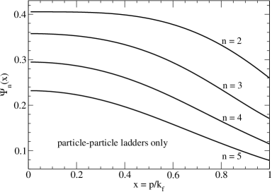
Figure 10: Momentum dependence of perturbative contributions to the real single-particle potential inside the Fermi sphere.

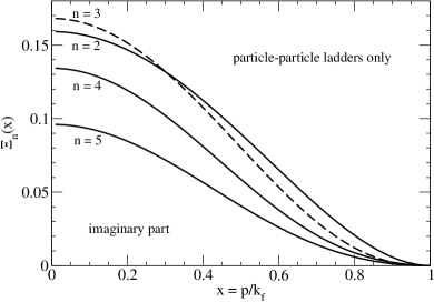
Figure 11: Momentum dependence of perturbative contributions to the imaginary single-particle potential inside the Fermi sphere.

The perturbative expansion of the complex single-particle potential $U(p,k_{f})+i\,W(p,k_{f})$ given in eqs.(43,44) has again the form:

$$U(p,k_{f})+i\,W(p,k_{f})={k_{f}^{2}\over 2M}\sum_{n=1}^{\infty}(-ak_{f})^{n}\Big{[}\Psi_{n}(x)+i\,\Xi_{n}(x)\Big{]}\,,$$ (46)

where e.g. the dimensionless functions $\Psi_{n}(x)$ for the real part can be calculated as:

$$\Psi_{n}(x)={16\over\pi^{n}}\int\limits_{0}^{1}\!ds\,s^{2}\!\!\int\limits_{0}^{\sqrt{1-s^{2}}}\!\!d\kappa\,\kappa\,F(s,\kappa)^{n-2}\Big{[}(n-1)\widehat{F}(s,\kappa,x)I(s,\kappa)+\widehat{I}_{*}(s,\kappa,x)F(s,\kappa)\Big{]}\,.$$ (47)

The functions at the lowest two orders are: $\Psi_{1}(x)=4/3\pi$, $\Xi_{1}(x)=0$ and $\Psi_{2}(x)=\Phi_{2}(x)$, $\Xi_{2}(x)=\Omega_{2}(x)$, with the analytical expressions for $\Phi_{2}(x)$ and $\Omega_{2}(x)$ written in eqs.(28,30) for $0<x<1$. These equalities come from the fact that hole-hole ladder diagrams [5] start to contribute to the energy density first at order $a^{3}$. One verifies that the double-integral representation of $\Psi_{2}(x)$ in eq.(47) gives results that are in perfect agreement with the analytical expression for $\Phi_{2}(x)$. Note that in the present calculation the identity $\Phi_{2}(x)=\Psi_{2}(x)$ is not self-evident, since different integrands $\widehat{R}(s,\kappa,x)I(s,\kappa)+\widehat{I}_{*}(s,\kappa,x)R(s,\kappa)\neq\widehat{F}(s,\kappa,x)I(s,\kappa)+\widehat{I}_{*}(s,\kappa,x)F(s,\kappa)$ are used to represent both functions.

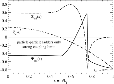
Figure 12: Momentum dependence of the single-particle potential inside the Fermi sphere in the limit $a\to\infty$.

The $x$-dependence of the functions $\Psi_{n}(x)$ and $\Xi_{n}(x)$ is shown for $n=2,3,4,5$ in Figs. 10,11. One observes monotonically decreasing functions of $x$ as well as a tendency that higher-orders get smaller in magnitude. Precise numerical values of the boundary values $\Psi_{n}(0)$, $\Xi_{n}(0)$ and $\Psi_{n}(1)$ are listed in Table 1 up to order $n=8$. The right boundary values are determined by the Hugenholtz-Van-Hove theorem as: $\Psi_{n}(1)=16(n+5)\pi^{-n}\int\!ds\,s^{2}\!\int\!d\kappa\,\kappa\,I(s,\kappa)F(s,\kappa)^{n-1}$. Note that for $n\geq 3$ the functions $\Phi_{n}(x)$ (shown in Fig. 4 are always larger than the functions $\Psi_{n}(x)$. At each order their difference is a measure of the additional contributions from the (combined) hole-hole ladder diagrams.

It is again straightforward to perform the limit $a\to-\infty$ of the single-particle potentials $U(p,k_{f})$ and $W(p,k_{f})$ given in eqs.(43,44). The corresponding results read:

$$U(p,k_{f})^{(\infty)}={8k_{f}^{2}\over M}\int\limits_{0}^{1}\!ds\,s^{2}\!\!\int\limits_{0}^{\sqrt{1-s^{2}}}\!\!d\kappa\,\kappa\,\Bigg{\{}{\widehat{F}(s,\kappa,x)I(s,\kappa)\over F(s,\kappa)^{2}}-{\widehat{I}_{*}(s,\kappa,x)\over F(s,\kappa)}\Bigg{\}}={k_{f}^{2}\over 2M}\,\Psi_{\rm uni}(x)\,,$$ (48)

$$W(p,k_{f})^{(\infty)}={8\pi k_{f}^{2}\over M}\int\limits_{0}^{1}\!ds\,s^{2}\!\!\int\limits_{0}^{\sqrt{1-s^{2}}}\!\!d\kappa\,\kappa\,{[\widehat{I}_{*}(s,\kappa,x)-\widehat{I}(s,\kappa,x)]I(s,\kappa)\over F(s,\kappa)^{2}}={k_{f}^{2}\over 2M}\,\Xi_{\rm uni}(x)\,,$$ (49)

where the functions $\Psi_{\rm uni}(x)$ and $\Xi_{\rm uni}(x)$ describe the dependence on the rescaled momentum variable $x=p/k_{f}$. The calculated boundary values are:

$$\Psi_{\rm uni}(0)=-0.451\,,\qquad\Psi_{\rm uni}(1)=\xi_{n}^{(pp)}-1=-0.763\,,\qquad\Xi_{\rm uni}(0)=0.587\,,$$ (50)

with $\xi_{n}^{(pp)}=0.237$ the normal Bertsch parameter [2, 5] obtained from the resummed particle-particle ladder diagrams. The $x$-dependence of the function $\Psi_{\rm uni}(x)$ is shown in Fig. 12. In the region $0.5<x<0.8$ one finds an extreme behavior. After a steep rise up to positive values of $0.58$ follows a discontinuous drop-back to negative values at $x=0.75$. It is a challenge to evaluate with good numerical accuracy the integrals over the regularized double-pole in eq.(48). However, the employed methods  showed good convergence in the range $\epsilon=10^{-2}\dots 10^{-3}$ of the regulator parameter and could be successfully tested with analytically solvable examples. The prompt reproduction of the relation $\Psi_{\rm uni}(1)=\xi_{n}^{(pp)}-1$ as imposed by the Hugenholtz-Van-Hove theorem is a further test of the quality of the numerical methods. The negative slope of $\Psi_{\rm uni}(x)$ at $x=1$ translates into a slightly enhanced effective mass: $M^{*}/M=[1+\Psi^{\prime}_{\rm uni}(1)/2]^{-1}\simeq 1.2$. The average value of $\Psi_{\rm uni}(x)$ taken over the interior of the Fermi sphere is: $3\int_{0}^{1}dx\,x^{2}\Psi_{\rm uni}(x)=-48\int ds\,s^{2}\int d\kappa\,\kappa\,I_{*}R/F^{2}=-0.433$. This is rather close to the value $\Psi_{\rm uni}(0)=-0.451$ at the bottom of the Fermi sea. The dashed line in Fig. 12 shows the $x$-dependence of the function $\Xi_{\rm uni}(x)$ associated with the imaginary potential. While having positive values over a wide range in $x$, it changes its sign in the vicinity of the point where $\Psi_{\rm uni}(x)$ has a discontinuity. In the calculation the negative values of $\Xi_{\rm uni}(x)$ result from treatment of the double-pole $1/F(s,\kappa)^{2}$ in eq.(49) as a regularized distribution. It should be stressed that the same regularization in the case of the real part $U(p,k_{f})^{(\infty)}$ reproduces the relation $\Psi_{\rm uni}(1)=\xi_{n}^{(pp)}-1$ as imposed by the Hugenholtz-Van-Hove theorem. The negative values of $\Xi_{\rm uni}(x)$ for $0.74<x<1$ imply an instability of the system against excitations of hole states in the Fermi sea. This instability should be viewed as a failure of the truncation to particle-particle ladder diagrams only. Moreover, there exists the momentum region $0.61<x<0.76$ inside which $\Psi_{\rm uni}(x)>\xi_{n}^{(pp)}-x^{2}$ holds and an instability to bubble formation in the Fermi sea occurs.

3.2 Continuation into region outside the Fermi sphere

In this subsection we present the modifications of the formalism that are necessary in order to continue the complex single-particle potential $U(p,k_{f})+i\,W(p,k_{f})$ generated by the particle-particle ladder diagrams into the region $p>k_{f}$ outside the Fermi sphere.

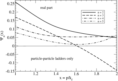
Figure 13: Momentum dependence of perturbative contributions to the real single-particle potential outside the Fermi sphere.

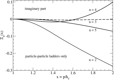
Figure 14: Momentum dependence of perturbative contributions to the imaginary single-particle potential outside the Fermi sphere.

Viewed as a weighting function for integrals over $\theta(k_{f}-|\vec{p}_{1}|)\,\delta^{3}(\vec{p}_{2}-\vec{p}\,)$, the support of the function $\widehat{I}_{*}(s,\kappa,x)$ consists for $x>1$ only of a circular wedge (defined by the inequalities $s+\kappa>x$ and $s^{2}+\kappa^{2}<(x^{2}+1)/2$). Consequently, this function takes for $x>1$ the simpler form:

$$\widehat{I}_{*}(s,\kappa,x)={1\over sx}\,\theta(s+\kappa-x)\,\theta(1+x^{2}-2(s^{2}+\kappa^{2}))\,.$$ (51)

The largest possible values of $s$ and $\kappa$ are now $s_{+}=\kappa_{+}=(x+1)/2>1$. For values $s>1$ the two Fermi spheres, which define the integration region of the in-medium loop $B_{p}$ in eq.(36), are no longer overlapping but get completely separated. This implies a change in the lower integration boundaries of both the radial and angular coordinates of $\vec{l}$. Taking into account the modifications which occur for $s>1$, the extended function $F(s,\kappa)$ reads:

$$F(s,\kappa) = 1+s-\kappa\ln{1+s+\kappa\over 1+s-\kappa}+{1\over 2s}(1-s^{2}-\kappa^{2})\ln{(1+s)^{2}-\kappa^{2}\over|s^{2}+\kappa^{2}-1|}$$ (52)

$$+\,\theta(s-1)\,\Bigg{\{}1-s+\kappa\ln{|s+\kappa-1|\over|s-\kappa-1|}+{1\over 2s}(s^{2}+\kappa^{2}-1)\ln{|(s-1)^{2}-\kappa^{2}|\over|s^{2}+\kappa^{2}-1|}\Bigg{\}}\,.$$

Actually, for $s>1$ the equality $F(s,\kappa)=R(s,\kappa)$ holds (see eq.(6)). The other function $\widehat{F}(s,\kappa,x)$ changes also when $x>1$, and its continued version reads:

$$\widehat{F}(s,\kappa,x)={1\over sx}\Bigg{\{}\theta(x-2s-1)\ln{|(s+x)^{2}-\kappa^{2}|\over|(s-x)^{2}-\kappa^{2}|}+\theta(2s+1-x)\ln{2|(s+x)^{2}-\kappa^{2}|\over|1+x^{2}-2(s^{2}+\kappa^{2})|}\Bigg{\}}\,.$$ (53)

Note that the distinction of cases $0<s<1/2$ and $1/2<s<1$ is no longer necessary, since the case $x<1-2s$ becomes inapplicable when $x>1$. Returning to the resummed interaction density $V_{p}(\tilde{\eta})$ in eq.(39) and using the two extended functions $F(s,\kappa)$ and $\widehat{F}(s,\kappa,x)$, the continuation of the complex single-particle potential $U(p,k_{f})+i\,W(p,k_{f})$ into the region $p>k_{f}$ outside the Fermi sphere takes the form:

$$U(p,k_{f}) = {8ak_{f}^{3}\over M}\int\limits_{0}^{(x+1)/2}\!ds\,s^{2}\!\!\int\limits_{0}^{(x+1)/2}\!\!d\kappa\,\kappa\,\Bigg{\{}{ak_{f}\widehat{F}(s,\kappa,x)I_{*}(s,\kappa)\over[\pi+ak_{f}F(s,\kappa)]^{2}}-{\widehat{I}_{*}(s,\kappa,x)\,\theta(1-s^{2}-\kappa^{2})\over\pi+ak_{f}F(s,\kappa)}$$ (54)

$$\qquad\qquad\qquad\qquad\qquad\qquad-\,{\widehat{I}_{*}(s,\kappa,x)[\pi+ak_{f}F(s,\kappa)]\,\theta(s^{2}+\kappa^{2}-1)\over[\pi+ak_{f}F(s,\kappa)]^{2}+[ak_{f}\pi\,I(s,\kappa)]^{2}}\Bigg{\}}\,,$$

$$W(p,k_{f})=-{8\pi a^{2}k_{f}^{4}\over M}\int\limits_{0}^{(x+1)/2}\!ds\,s^{2}\!\!\int\limits_{0}^{(x+1)/2}\!\!d\kappa\,\kappa\,{\widehat{I}_{*}(s,\kappa,x)I(s,\kappa)\,\theta(s^{2}+\kappa^{2}-1)\over[\pi+ak_{f}F(s,\kappa)]^{2}+[ak_{f}\pi\,I(s,\kappa)]^{2}}\,.$$ (55)

Note that the imaginary part Im $\bar{B}_{p}=ak_{f}[I(s,\kappa)-I_{*}(s,\kappa)]$ at $\tilde{\eta}=0$, which is nonzero only for $s^{2}+\kappa^{2}>1$, affects both the real and the imaginary single-particle potential outside the Fermi sphere. The last term in eqs.(54,55) indicates that the complex denominator $\pi+ak_{f}[F(s,\kappa)-i\pi\,I(s,\kappa)]$ has been involved in the derivation.

We first analyze the continuation of $U(p,k_{f})+i\,W(p,k_{f})$ into the region $p>k_{f}$ according to the perturbative expansion in eq.(46). For the contribution at second order one has again the equalities: $\Psi_{2}(x)=\Phi_{2}(x)$ and $\Xi_{2}(x)=\Omega_{2}(x)$, with the corresponding analytical expressions for $x>1$ given in eqs.(29,30). The double-integral representation of the function $\Psi_{2}(x)$ for $x>1$ as obtained by expanding eq.(54) to second order in $ak_{f}$ leads to results which are in perfect numerical agreement with $\Phi_{2}(x)$ written in eq.(29). This consistency serves as an important check on the formalism (i.e. modified functions $F(s,\kappa)$ and $\widehat{F}(s,\kappa,x)$) employed in the continuation of the complex single-particle potential $U(p,k_{f})+i\,W(p,k_{f})$ into the region $p>k_{f}$. The $x$-dependence of the functions $\Psi_{n}(x)$ and $\Xi_{n}(x)$ with $n=2,3,4,5$ is shown in Figs. 13,14 for $1<x<2$. One observes a behavior quite similar to that of the functions $\Phi_{n}(x)$ and $\Omega_{n}(x)$ shown in Figs. 6,7. This means that the additional (combined) hole-hole ladder diagrams have little influence on the properties of particle excitations outside the Fermi sphere.

Finally, the continuation of the functions $\Psi_{\rm uni}(x)$ and $\Xi_{\rm uni}(x)$ describing the momentum dependence of the complex single-particle potential in the limit $a\to\infty$ is shown in Fig. 15 for $1<x<3$. Again, some non-trivial numerics is involved in producing the curve for $\Psi_{\rm uni}(x)$ in Fig. 15. One observes a fast decrease of the attractive real part in the region $1<x<2$. Particle excitations with higher momentum $x>2.1$ experience a weak repulsion from the fermionic medium. The behavior of the function $\Xi_{\rm uni}(x)$ for $x>1$ is very similar to that of $\Omega_{\rm uni}(x)$ shown in Fig. 9. In fact for $x\geq 3$ both functions become equal: $\Xi_{\rm uni}(x)=\Omega_{\rm uni}(x)$. The reason for this equality is that for $x>3$ only values of $s>(x-1)/2>1$ contribute to the double-integral. Under this condition one has $F(s,\kappa)=R(s,\kappa)$ and the representations of $W(p,k_{f})$ in eqs.(21,55) coincide with each other. It should be noted that the negative values of $\Xi_{\rm uni}(x)$ for $x>1$ ensure the stability of particle excitations outside the Fermi sphere. When approaching the Fermi surface from the right, the (negative) slope $\Xi^{\prime}_{\rm uni}(1^{\!+})=-8\pi(1-s_{1})s_{1}^{2}=-2.4819$ (with $s_{1}=0.40865$) is found. At finite coupling strength $ak_{f}$, one obtains for the left and right slope of the function $\Xi(x)=2Mk_{f}^{-2}\,W(p,k_{f})$ at the Fermi surface $x=1$:

$$\Xi^{\prime}(1^{\!-})=0\,,\qquad\Xi^{\prime}(1^{\!+})=-{8\pi s_{1}^{2}(1-s_{1}^{2})\over 1+s_{1}+\pi(ak_{f})^{-1}s_{1}^{2}}\,,$$ (56)

where $s_{1}$ is the solution of the equation $F(s_{1},\sqrt{1-s_{1}^{2}})=-\pi/ak_{f}$. The largest negative slope $\Xi^{\prime}(1^{\!+})\simeq-8\pi/3$ is reached for $ak_{f}\simeq-\pi/2$ (approached from below).

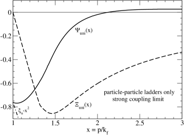
Figure 15: Momentum dependence of the single-particle potential outside the Fermi sphere in the limit $a\to\infty$.

Furthermore, we have extended the construction of the complex single-particle potential $U(p,k_{f})+i\,W(p,k_{f})$ to the hole-hole ladder diagrams [5]. At leading order $a^{3}$, one obtains precisely the difference between the third order results in section 2 and section 3, proportional to $(-ak_{f})^{3}$. Beyond that order mixed ladder diagrams with so far unknown systematics appear.

4 Single-particle potential from ring diagrams

In this section we calculate the on-shell single-particle potential which arises from the particle-hole ring diagrams generated by a contact-interaction proportional to the scattering length $a$. We follow the method to treat ring diagrams as described in the text book by Gross, Runge and Heinonen [17]. The key quantity is the (euclidean) polarization function:

$$B_{\rm ring}=8\pi a\int\!\!{d^{3}l\over(2\pi)^{3}}\,{2\vec{l}\cdot\vec{q}\over(\vec{l}\cdot\vec{q}\,)^{2}+M^{2}\omega^{2}}\,N_{\eta}(\vec{l}-\vec{q}/2,\vec{p}\,)\Big{[}1-N_{\eta}(\vec{l}+\vec{q}/2,\vec{p}\,)\Big{]}\,,$$ (57)

where the integrand is the Fourier transform of the exponential term in eq.(22.15) of ref.[17] and the factor $N_{\eta}(\dots)[1-N_{\eta}(\dots)]$ incorporates the pertinent integration boundaries together with the perturbation by the test-particle of momentum $\vec{p}$. Averaging over the directions of $\vec{p}$, one gets to linear order in the parameter $\tilde{\eta}=\eta\,\pi^{2}/k_{f}^{3}$:

$$\bar{B}_{\rm ring}={2ak_{f}\over\pi}\Big{\{}Q(s,\kappa)+\tilde{\eta}\,\widehat{Q}(s,\kappa,x)\Big{\}}\,\,,$$ (58)

where the momenta have been set to $|\vec{q}\,|=2sk_{f}$ and $|\vec{p}\,|=xk_{f}$, and the frequency to $\omega=2s\kappa k_{f}^{2}/M$. The first function introduced in eq.(58) has the well-known form [17]:

$$Q(s,\kappa)=1-\kappa\arctan{1+s\over\kappa}-\kappa\arctan{1-s\over\kappa}+{1\over 4s}(1-s^{2}+\kappa^{2})\ln{(1+s)^{2}+\kappa^{2}\over(1-s)^{2}+\kappa^{2}}\,,$$ (59)

and its values lie in the range $0<Q(s,\kappa)\leq 2$. The correction term linear in $\tilde{\eta}$ is determined by the second function:

$$\widehat{Q}(s,\kappa,x)={1\over 2sx}\ln{(s+x)^{2}+\kappa^{2}\over(s-x)^{2}+\kappa^{2}}\,,\qquad\qquad\widehat{Q}(s,\kappa,0)={2\over s^{2}+\kappa^{2}}\,.$$ (60)

An interesting relation between these two functions is: $\int_{0}^{1}dx\,x^{2}\widehat{Q}(s,\kappa,x)=Q(s,\kappa)$. It is worth mentioning that exactly the same result for $\bar{B}_{\rm ring}$ is obtained, if the last factor $1-N_{\eta}(\dots)$ in eq.(57) is dropped. Such a simpler representation of the polarization function $B_{\rm ring}$ can be derived in the finite temperature formalism when taking the limit $T\to 0$ in the end.

The interaction energy per particle arising from the leading $n$-ring diagram (with a spin-factor $2^{n}$) is given by the expression:

$$\bar{E}(k_{f})^{n-\rm ring}=-{12k_{f}^{2}\over\pi Mn}\bigg{(}{2ak_{f}\over\pi}\bigg{)}^{\!n}\int\limits_{0}^{\infty}\!ds\,s^{3}\int\limits_{0}^{\infty}\!d\kappa\,\big{[}Q(s,\kappa)\big{]}^{n}={k_{f}^{2}\over 2M}(ak_{f})^{n}\,\Gamma_{n}\,.$$ (61)

All the additional exchange-type diagrams due to the Pauli exclusion-principle can be taken into account simply by replacing the factor $2^{n}$ by the proper spin-factor $S_{n}=1+3(-1)^{n}$ [5]. Starting at third order and going up to 8-th order, the numerical values of the coefficients $\Gamma_{n}$ are: $\Gamma_{3}=-0.22955$, $\Gamma_{4}=-0.069116$, $\Gamma_{5}=-0.038274$, $\Gamma_{6}=-0.025904$, $\Gamma_{7}=-0.019548$, $\Gamma_{8}=-0.015841$. Note that these coefficients are all negative and they decrease in magnitude.

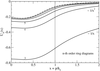
Figure 16: Momentum dependence of contributions from particle-hole ring diagrams to the real single-particle potential.

Since the interaction density of a $n$-ring diagram is completely determined by the $n$-th power of the polarization bubble $\bar{B}_{\rm ring}$ the expression for the on-shell single-particle potential follows as:

$$U(p,k_{f})^{n-\rm ring}=-{4k_{f}^{2}\over\pi M}\bigg{(}{2ak_{f}\over\pi}\bigg{)}^{\!n}\int\limits_{0}^{\infty}\!ds\,s^{3}\int\limits_{0}^{\infty}\!d\kappa\,\widehat{Q}(s,\kappa,x)\big{[}Q(s,\kappa)\big{]}^{n-1}={k_{f}^{2}\over 2M}(ak_{f})^{n}\,U_{n}(x)\,,$$ (62)

where the dimensionless function $U_{n}(x)$ describes the momentum dependence at $n$-th order.

Fig. 16 shows the calculated potential-functions $U_{n}(x)$ in the region $0<x<2$ from third up to 8-th order. One observes an almost constant behavior in the region $0<x<0.4$ that is followed by a steady increase and an asymptotic approach to zero. The detailed asymptotic behavior of the functions $U_{n}(x)$ for large $x$ is: $U_{3}(x)\simeq-16(4+\pi^{2})/(9\pi^{3}x)\simeq-0.79523/x$ and $U_{n}(x)\simeq 4(n-1)\Gamma_{n-1}/(3\pi x^{2})$ for $n\geq 4$. The Hugenholtz-Van-Hove theorem is fulfilled order by order in the form of the relation $U_{n}(1)=\Gamma_{n}(n+5)/3$, which holds with very good numerical accuracy. Another interesting property is given by the relation $3\int_{0}^{1}dx\,x^{2}U_{n}(x)=n\Gamma_{n}$. Such a connection between the single-particle potential and the contribution to $\bar{E}(k_{f})$ is typical for an $n$-body interaction treated at first order in perturbation theory [11]. The absence of an imaginary single-particle potential $W(p,k_{f})$ from particle-hole ring diagrams is also remarkable. We do not study here in further detail the resummation of ring diagrams to all orders since for this subclass the limit $a\to-\infty$ does not exist.

Appendix: Resummation of in-medium ladder diagrams in two dimensions

In this appendix we present the resummation of fermionic in-medium ladder diagrams to all orders in two spatial dimensions. The derivation follows essentially the same steps as in the case of the three-dimensional calculation presented in detail in ref.[2].

For a system of spin-1/2 fermions in two dimensions the relation between particle density (per area) and Fermi momentum is $\rho_{2}=k_{f}^{2}/2\pi$. Likewise, the free Fermi gas energy per particle is $\bar{E}(k_{f})^{(0)}=k_{f}^{2}/4M$, with $M$ the large fermion mass. We introduce a two-body contact-interaction with coupling constant $C_{0}=2\pi\alpha/M$, where $\alpha$ is a dimensionless parameter. The corresponding first-order Hartree-Fock contribution is readily calculated as: $\bar{E}(k_{f})^{(1)}=-\alpha\,k_{f}^{2}/4M$. The calculation of higher-order contributions from ladder diagrams and their eventual resummation to all orders requires the knowledge of the complex-valued in-medium loop $B_{0}^{\prime}+B_{1}^{\prime}+B_{2}^{\prime}$ in two dimensions. The rescattering term $B_{0}^{\prime}$ in vacuum (with zero medium-insertions) is given by the expression:

$$B_{0}^{\prime}=2\pi\alpha\int\!\!{d^{2}l\over(2\pi)^{2}}\,{1\over\vec{l}^{\,2}-\vec{q}^{\,2}-i\epsilon}=\alpha\bigg{(}{i\pi\over 2}-\ln{|\vec{q}\,|\over\Lambda}\bigg{)}\,,$$ (63)

with $\Lambda$ an ultraviolet cutoff. The bound-state pole in the resummed vacuum scattering amplitude $\alpha/(1-B_{0}^{\prime})$ fixes the value of the cutoff $\Lambda$. By solving the equation $B_{0}^{\prime}=1$ one gets $\Lambda=q_{b}\,e^{1/\alpha}$, where $q_{b}$ is the binding momentum related to the two-body binding energy by $E_{b}=-q_{b}^{2}/M<0$. The contribution $B_{1}^{\prime}$ from the diagrams with one medium-insertion (see Fig. 1) has a real part of the form:

$${\rm Re}\,B_{1}^{\prime} = -2\pi\alpha\int\!\!{d^{2}l\over(2\pi)^{2}}\,{1\over\vec{l}^{\,2}-\vec{q}^{\,2}}\Big{[}\theta(k_{f}-|\vec{P}+\vec{l}\,|)+\theta(k_{f}-|\vec{P}-\vec{l}\,|)\Big{]}$$ (64)

$$= -\alpha\,{\rm Re}\!\int_{0}^{1}\!d\lambda\,{{\rm sign}(\lambda+s^{2}-\kappa^{2})\over\sqrt{[\lambda-(s+\kappa)^{2}][\lambda-(s-\kappa)^{2}]}}=\alpha\,\Big{\{}\ln\kappa-H(s,\kappa)\Big{\}}\,,$$

where we have displayed in the second line the intermediate result obtained after angular integration. Here, $\vec{P}=(\vec{p}_{1}+\vec{p}_{2})/2$ and $\vec{q}=(\vec{p}_{1}-\vec{p}_{2})/2$ are the half-sum and half-difference of two two-component momenta $|\vec{p}_{1,2}|<k_{f}$ inside a Fermi disc. The dimensionless variables $s=P/k_{f}$ and $\kappa=q/k_{f}$ satisfy the constraint $s^{2}+\kappa^{2}<1$. The radial integral in eq.(64) can be solved in terms of a piecewise defined logarithmic function:

$$H(s,\kappa)=2\,\theta(1-s-\kappa)\ln{\sqrt{1-(s+\kappa)^{2}}+\sqrt{1-(s-\kappa)^{2}}\over 2\sqrt{\kappa}}+\theta(s+\kappa-1)\ln s\,.$$ (65)

The imaginary part of the in-medium loop in two dimensions has the form:

$${\rm Im}(B_{0}^{\prime}+B_{1}^{\prime}+B_{2}^{\prime}) = 2\pi^{2}\alpha\int\!\!{d^{2}l\over(2\pi)^{2}}\,\delta(\vec{l}^{\,2}-\vec{q}^{\,2})\,\theta(k_{f}-|\vec{P}+\vec{l}\,|)\,\theta(k_{f}-|\vec{P}-\vec{l}\,|)$$ (66)

$$= {B_{2}^{\prime}\over 2i}=\alpha\,J(s,\kappa)\,.$$

where we have already dropped an analogous term proportional to $[1-\theta(\dots)]\,[1-\theta(\dots)]$, since its phase space vanishes identically by Pauli-blocking and energy conservation (see herefore the detailed discussion in section 3 of ref.[2]). In a geometrical picture the function $4J(s,\kappa)$ measures the arc length of a circle inside the intersection of two shifted circular discs and it reads:

$$J(s,\kappa)={\pi\over 2}\,\theta(1-s-\kappa)+\theta(s+\kappa-1)\arcsin{1-s^{2}-\kappa^{2}\over 2s\kappa}\,.$$ (67)

It is interesting to note that $s\kappa J(s,\kappa)$ serves also as a weighting function for integrals over the product of two Fermi discs:

$$\int\limits_{|\vec{p}_{1,2}|<k_{f}}\!\!\!\!{d^{2}p_{1}d^{2}p_{2}\over(2\pi)^{4}}\,f(s,\kappa)={2k_{f}^{4}\over\pi^{3}}\int\limits_{0}^{1}\!ds\,s\!\!\int\limits_{0}^{\sqrt{1-s^{2}}}\!\!d\kappa\,\kappa\,J(s,\kappa)\,f(s,\kappa)\,,$$ (68)

where the integrand depends on $s=|\vec{p}_{1}+\vec{p}_{2}|/2k_{f}$ and $\kappa=|\vec{p}_{1}-\vec{p}_{2}|/2k_{f}$. Following the instructive diagrammatic analysis in section 4 of ref.[2] one arrives with these ingredients at the following result for resummed interaction energy per particle from ladder diagrams:

$$\bar{E}(k_{f})=-{8k_{f}^{2}\over\pi M}\int\limits_{0}^{1}\!ds\,s\!\!\int\limits_{0}^{\sqrt{1-s^{2}}}\!\!d\kappa\,\kappa\,\arctan{J(s,\kappa)\over H(s,\kappa)+\ln(k_{f}/q_{b})}\,.$$ (69)

Note that either the parameter $\alpha$ or the cutoff $\Lambda$ have dropped out in the above ratio, since according the relation $\alpha^{-1}+\ln(k_{f}/\Lambda)=\ln(k_{f}/q_{b})$ only the binding momentum $q_{b}$ remains as a physically relevant scale parameter. The dependence of $\bar{E}(k_{f})$ on the dimensionless strength parameter $\gamma=\ln(k_{f}/q_{b})$ can be analyzed for large values of $\gamma$ in the form of a power series in $\gamma^{-1}$, which reads:

$$\bar{E}(k_{f})={k_{f}^{2}\over 4M}\bigg{\{}-\gamma^{-1}+\bigg{(}{3\over 4}-\ln 2\bigg{)}\gamma^{-2}-0.16079\,\gamma^{-3}-0.06009\,\gamma^{-4}-0.13832\,\gamma^{-5}+\dots\bigg{\}}\,.$$ (70)

When setting $\Lambda=k_{f}$ the expansion in powers of $\gamma^{-1}$ becomes equivalent to the weak coupling expansion in powers of $\alpha$. This way one recovers the earlier mentioned first-order Hartree-Fock result. Remarkably, the coefficient at second order $\gamma^{-2}$ can be calculated exactly with the (small) value $3/4-\ln 2=0.056853$.

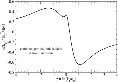
Figure 17: Interaction energy per particle $\bar{E}(k_{f})$ divided by the free Fermi gas energy $k_{f}^{2}/4M$ in two dimensions as a function of the parameter $\gamma=\ln(k_{f}/q_{b})$.

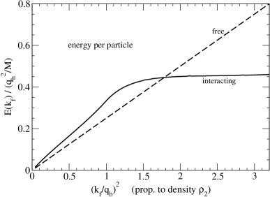
Figure 18: Equation of state of a two-dimensional Fermi gas resulting from the resummation of ladder diagrams to all orders.

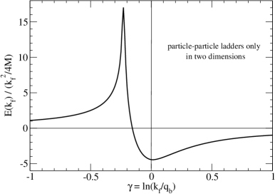
Figure 19: Ratio of interaction energy per particle $\bar{E}(k_{f})$ and free Fermi gas energy $k_{f}^{2}/4M$ as a function of the parameter $\gamma=\ln(k_{f}/q_{b})$. Only the particle-particle ladder diagrams are considered.

The ratio between the interaction energy per particle $\bar{E}(k_{f})$ and the free Fermi gas energy $k_{f}^{2}/4M$ is shown in Fig. 17 as a function of the dimensionless strength parameter $\gamma=\ln(k_{f}/q_{b})$. One observes an oscillatory behavior with moderate repulsion for $\gamma<0.29$ and somewhat stronger attraction for $\gamma>0.29$. The asymptotic expansion in eq.(70) provides a very good approximation of the ratio $4M\bar{E}(k_{f})/k_{f}^{2}$ for the values $|\gamma|>4$ outside the plotted range. The positive and negative areas above and below the $\gamma$-axis in Fig. 17 compensate each other exactly. In Fig. 18 the equation of state of a free and an interacting two-dimensional Fermi gas are directly compared with each other. The variable $(k_{f}/q_{b})^{2}$ on the abscissa is now directly proportional to the density $\rho_{2}=k_{f}^{2}/2\pi$. One observes weak repulsion in the low-density regime and sizeable attraction above a critical density $\rho_{c}\simeq 0.28M|E_{b}|$ that is determined by the two-body binding energy .

For the sake of completeness we consider also the particle-particle ladder diagrams in two dimensions. The resummation to all orders leads to a geometrical series and the corresponding interaction energy per particle is given by the expression:

$$\bar{E}(k_{f})=-{8k_{f}^{2}\over\pi M}\int\limits_{0}^{1}\!ds\,s\!\!\int\limits_{0}^{\sqrt{1-s^{2}}}\!\!d\kappa\,\kappa\,{J(s,\kappa)\over H_{p}(s,\kappa)+\ln(k_{f}/q_{b})}\,,$$ (71)

with the two-dimensional bubble function:

$$H_{p}(s,\kappa)={1\over\pi}\int_{0}^{\pi/2}\!d\varphi\ln\Big{[}\Big{(}s\cos\varphi+\sqrt{1-s^{2}\sin^{2}\varphi}\Big{)}^{2}-\kappa^{2}\Big{]}\,.$$ (72)

Note that the condition $\kappa^{2}<1-s^{2}$ ensures that the argument of the logarithm is always positive. Although $H_{p}(s,\kappa)$ cannot be expressed in terms of elementary functions, the following relation holds: $H_{p}(s,\kappa)+{\rm Re}\,H_{p}(-s,\kappa)=H(s,\kappa)+\ln\kappa$, with $H(s,\kappa)$ written in eq.(65). The weak coupling expansion of $\bar{E}(k_{f})$ in eq.(71) has the form:

$$\bar{E}(k_{f})={k_{f}^{2}\over 4M}\bigg{\{}-\gamma^{-1}+\bigg{(}{3\over 4}-\ln 2\bigg{)}\gamma^{-2}-0.03147\,\gamma^{-3}-0.004415\,\gamma^{-4}-0.005598\,\gamma^{-5}+\dots\bigg{\}}\,,$$ (73)

with $\gamma=\ln(k_{f}/q_{b})$. Obviously, the first two terms agree with eq.(70) and the different coefficients of the higher order terms indicate the influence of the hole-hole ladder diagrams. Fig. 19 shows the ratio of the interaction energy per particle $\bar{E}(k_{f})$ divided by the free Fermi gas energy $k_{f}^{2}/4M$ in the range $-1<\gamma<1$. For $|\gamma|>1$ the asymptotic expansion in eq.(73) provides a very good approximation of the $\gamma$-dependence. The sharp peak at $\gamma\simeq-0.23$ and large magnitude of the ratio in comparison to Fig. 17 should be considered as an artefact of the truncation to particle-particle ladder diagrams. The areas above and below the $\gamma$-axis again compensate each other exactly. It is a generic feature that the truncation to particle-particle ladder diagrams develops a much stronger dependence on a control parameter than the complete (particle and hole) ladder series. A further example for this fact is the energy per particle from a resummed p-wave contact-interaction shown in Fig. 5 of ref.[7]. Throughout this work the results obtained from the complete (particle and hole) ladder series are the ones with the higher priority.

References

- [1] W. Zwerger (Editor), “BCS-BEC Crossover and Unitary Fermi Gas”, in Lect. Notes Phys. 836 (Springer, 2012).
- [2] N. Kaiser, Nucl. Phys. A 860, 41 (2005).
- [3] H.W. Hammer and R.J. Furnstahl, Nucl. Phys. A 678, 277 (2000).
- [4] J.V. Steele, nucl-th/0010066. The middle term in eq.(16) needs to be corrected and multiplied by a factor 2 (confirmed by H.W. Hammer).
- [5] T. Schäfer, C.W. Kao and S.R. Cotanch, Nucl. Phys. A 762, 82 (2005).
- [6] M.J.H. Ku, A.T. Sommer, L.W. Cheuk and M.W. Zwierlein, Nature Phys. 8, 366 (2012); cond-mat/1110.3309.
- [7] N. Kaiser, Eur. Phys. J. A 48, 148 (2012).
- [8] G. Sarma, J. Phys. Chem. Solids 24 1029 (1963).
- [9] P. Magierski, G. Wlazlowski, A. Bulgac and J.E. Drut, Phys. Rev. Lett. 103, 210403 (2009).
- [10] J.W. Holt, N. Kaiser, G.A. Miller and W. Weise, Phys. Rev. C 88, 024614 (2013).
- [11] N. Kaiser, S. Fritsch and W. Weise, Nucl. Phys. A 700, 343 (2002).
- [12] J.M. Luttinger, Phys. Rev. 121, 942 (1961).
- [13] N.M. Hugenholtz and L. Van Hove, Physica 24, 363 (1958).
- [14] V.M. Galitskii, Sov. Phys. JEPT 7, 104 (1958).
- [15] G.E. Volovik, “Quantum Phase Transition from Topology in Momentum Space”, in Lect. Notes Phys. 718 (Springer, 2007).
- [16] S.S. Pankratov, M. Baldo and M.V. Zverev, Phys. Rev. C 86, 045804 (2012).
- [17] E.K.U. Gross, E. Runge and O. Heinonen, “Many-Particle Theory”, IOP Publishing Ltd, Bristol (1991); chapt. 22.