Simultaneous XMM-Newton and HST-COS observation of 1H0419-577:

In this paper we analyze the X-ray, UV and optical data of the Seyfert 1.5 galaxy 1H0419-577, with the aim of detecting and studying an ionized-gas outflow. The source was observed simultaneously in the X-rays with  XMM-Newton and in the UV with  HST-COS. Optical data were also acquired with the  XMM-Newton Optical Monitor. We detected a thin, lowly ionized warm absorber ($\log\xi\approx 0.03$, $\log\hbox{ $N{\rm{}_{H}}$ }\approx 19.9$ cm^-2) in the X-ray spectrum, consistent to be produced by the same outflow already detected in the UV. Provided the gas density estimated in the UV, the outflow is consistent to be located in the host galaxy, at $\approx$ kpc scale. Narrow emission lines were detected in the X-rays, in the UV and also in the optical spectrum. A single photoionized-gas model cannot account for all the narrow lines emission, indicating that the narrow line region is probably a stratified environment, differing in density and ionization. X-ray lines are unambiguously produced in a more highly ionized gas phase than the one emitting the UV lines. The analysis suggests also that the X-ray emitter may be just a deeper portion of the same gas layer producing the UV lines. Optical lines are probably produced in another, disconnected gas system. The different ionization condition, and the $\approx$ pc scale location suggested by the line width for the narrow lines emitters, argue against a connection between the warm absorber and the narrow line region in this source.

1 Introduction

Active galactic nuclei (AGN) are believed to be powered by the accretion of matter onto a supermassive black hole (Antonucci 1993). Emission and absorption lines in AGN spectra are the signatures of a plasma photoionized by the central source. High-resolution spectral observations can probe the physical conditions in this gas, providing information about the interaction between AGN radiation and the surrounding environment.

A variety of emission lines with different width (from $10^{2}$ to $10^{4}$ km s^-1) can be identified in AGN type 1 spectra. The diverse line-broadenings reflect a different location of the emitting region: narrower lines are believed to originate in a region farther from the black hole ($\approx$100 pc), lower in density and in temperature than the broad-line region (BLR) where broader lines are emitted (Osterbrock 1989). Lines emission ranges from the optical (e.g. [O iii], hydrogen Balmer series) to the X-ray waveband (e.g O vii, O viii, Ne ix). Narrow lines may be more difficult to detect. For instance, in the UV, narrow lines (NL) from e.g. C iv, O vi are blended in a dominant broad component and difficult to disentangle (e.g. Kriss et al. 2011). In the soft X-ray the flux of any emission line is usually outshone by the underlying continuum and lines detection is favored by a temporary low-flux state of the source (e.g. NGC 4051, Nucita et al. 2010). Whether X-ray lines arise in the same gas emitting the longer-wavelength lines is an open issue that has been recently addressed through multiwavelength photoionization modeling. In the case of Mrk 279, X-ray broad lines are consistent to be produced in a highly-ionized skin of the UV and optical BLR (Costantini et al. 2007). Bianchi et al. (2006) found that a single medium, photoionized by the central continuum, may produce the [O iii] to soft X-ray ratio observed in spatially resolved images of the narrow line region (NLR).

Besides the lines-emitting plasma, another photoionized-gas component that can modify the spectra of type 1 AGN is a warm absorber (WA), intervening in the line of sight. WA are commonly detected in about half type 1 AGN (Crenshaw & Kraemer 1997; Piconcelli et al. 2005) via UV and/or X-ray absorption lines. These lines are usually blueshifted, (see Crenshaw et al. 2003) indicating a global outflow of the absorber. In the last ten years, multiwavelength UV-X-ray campaigns (see Costantini (2010) and references therein) have depicted the physical conditions in the outflowing gas with great detail. WA are multi-component winds spanning a wide range in ionization and in velocity (e.g. Kriss et al. 2011; Ebrero et al. 2011). X-ray spectra show the the most highly ionized lines (e.g from O vii, O viii and Ne ix), while a lower-ionization phase (e.g. C ii, Mg ii) is visible only in the UV. In some cases (e.g. NGC 3783, NGC 5548, NGC 4151, Mrk 279), a common phase producing e.g. O vi lines both in the UV and in the X-ray spectrum has been identified (Kaspi et al. 2002; Steenbrugge et al. 2005; Kraemer et al. 2005; Arav et al. 2007). Similarities in the line width (NGC 3783, Behar et al. 2003) and in the gas column density (NGC 5548, Detmers et al. 2009) suggests a connection between the WA and the gas in the NLR. However, the origin of WA is not clearly established yet, mainly because of the great uncertainty in estimating its location.

Provided the gas density, the distance of the outflow from the central source can be in principle derived from the gas ionization parameter $\xi=L_{\rm ion}/nR^{2}$ (where $L_{\rm ion}$ is the source ionizing luminosity, $n$ is the gas density, and $R$ is the distance from the ionizing source). However, in most cases the gas density is unknown and the distance may just be estimated indirectly (Blustin et al. 2005). Absorption lines from collisionally-excited metastable levels may provide a direct density diagnostic (e.g. Bautista et al. 2009), but they are rarely detected. In the UV, metastable lines from e.g. Fe ii Si ii and C ii have been detected in a handful of cases (e.g. Moe et al. 2009; Dunn et al. 2010; Borguet et al. 2012). In the X-rays the identification of metastable lines from O v is hampered by uncertainties in the predicted line wavelength (Kaastra et al. 2004). So far, available estimations, using different methods, have located the outflows within the BLR (e.g. NGC 7469, Scott et al. 2005) or as far as the putative torus (e.g. Ebrero et al. 2010). In some quasars a galactic-scale distance have been reported. (Hamann et al. 2001; Hutsemékers et al. 2004; Borguet et al. 2012; Moe et al. 2009).

The distance estimation allows to quantify the amount of mass and energy released by the outflow into the medium. Hence, it is possible to establish if WA contribute in the so-called AGN feedback, which is often invoked to explain the energetics and and the chemistry of the medium up to a very large scale (Sijacki et al. 2007; Hopkins et al. 2008; Somerville et al. 2008; McNamara & Nulsen 2012). Warm absorbers usually produce a negligible feedback (e.g. Ebrero et al. 2011). Only the fastest AGN wind (e.g. Moe et al. 2009; Dunn et al. 2010; Tombesi et al. 2012), may be dynamically important in the evolution of the interstellar medium (Faucher-Giguère & Quataert 2012).

In this paper we analyze a long-exposure  XMM-Newton dataset of the bright Seyfert galaxy  1H0419-577 , taken simultaneously with a Cosmic Origins Spectrograph ( HST-COS ) spectrum. The source is a radio quiet quasar located at redshift z=0.104 and spectrally classified as a type 1.5 Seyfert galaxy (Véron-Cetty & Véron 2006). Using the H$\beta$ line width, Pounds et al. (2004b) derived a $1.3\times 10^{8}$ ${\rm M_{\odot}}$ mass for the supermassive black hole (SMBH) hosted in the nucleus. The HST-COS spectrum has been published by Edmonds et al. (2011, herafter E11). The UV spectrum displays broad emission lines from C iv, O vi, and  Ly$\rm{\,\sc{\alpha}}$ as well as absorption lines (E11). Three outflowing components were identified in absorption, with the line centroids located at $\rm v_{1}=-38\,\hbox{km s${}^{-1}$}$, $\rm v_{2}=-156\,\hbox{km s${}^{-1}$}$ and $\rm v_{3}=-220\,\hbox{km s${}^{-1}$}$ in the rest frame of the source. Only a few ionized species (H i, C iv, N v, O vi) were detected in component 1, while component 2+3 displays a handful of transitions from both low (e.g. C ii) and high-ionization species (e.g. C iv, N v, O vi).

The present analysis is focused mainly on the high-resolution spectrum collected with the Reflection Grating Spectrometer (RGS, den Herder et al. 2001); in a companion paper we will present the broad band X-ray spectrum of this source. Analysis of a previous RGS dataset is reported in Pounds et al. (2004a). Hints of narrow absorption features from an Fe unresolved transition array (UTA) were noticed in the spectrum. However, the short exposure time ($\approx 15$ ks) prevented so far an unambiguous detection and characterization of a warm absorber in this source.

The paper is organized as follows: in Sect. 2 we present the  XMM-Newton observations and the data reduction; in Sect. 3 we describe the spectral energy distribution of the source; in Sect. 4 we discuss the spectral analysis; in Sect. 5 we model the narrow emission lines of the source; in Sect. 6 we compare the X-ray and the UV absorber: finally in Sect. 7 we discuss our results and in Sect. 8 we present the conclusions. The cosmological parameter used are: $H_{0}$=70 km s^-1 Mpc^-1, $\Omega_{\rm m}$=0.3, $\Omega_{\Lambda}$=0.7. Errors are quoted at 68% confidence levels ($\Delta\chi^{2}=1.0$) unless otherwise stated.

2 Observations and data preparation

Table 1: XMM-Newton observation log for  1H0419-577 

Observation ID	0604720401	0604720301
Date	28/05/2010	30/05/2010
Orbit	1917	1918
Net exposure (ks)	61	97
RGS Count Rate ($\rm s^{-1}$)	$0.337\pm 0.002$	$0.385\pm 0.002$
EPIC-pn Count Rate ($\rm s^{-1}$)	$1.41\pm 0.02$	$1.56\pm 0.02$

In May 2010, two consecutive exposures of  1H0419-577 were taken with the  XMM-Newton X-ray telescope both with the EPIC cameras (Strüder et al. 2001; Turner et al. 2001) and the RGS. Moreover Optical Monitor (OM, Mason et al. 2001) Imaging Mode data were acquired with four broad-band filters (B, UVW1, UVM2, UWV2) and two grism filters (Grism1-UV and Grism2-visual). The source was observed for $\approx$ 167 ks in total and a slight shift in the dispersion direction was applied in the second observation. In this way, the bad pixels of the RGS detectors were not at the same location in the two observations, allowing us to correct them by a combination of the two spectra (see Sect. 2.1). Details of the two observations are provided in Table 1.

2.1 The RGS data

For both RGS datasets, we processed the data following the standard procedure , using the  XMM-Newton Science Analysis System (SAS, version 10.0.0) and the latest calibration files. We created calibrated event files for both RGS1 and RGS2, and to check the variation of the background, we created also the background light curves from CCD 9. The background of the first observation was quiescent, while the second light curve showed contamination by soft protons flares. We cleaned the contaminated observation applying a time filter to the event-files: for this purpose, we created the good time intervals (GTI) cutting in the light curve all the time bins where the count-rate was over the standard threshold of 0.2 counts s^-1. Resulting exposure time after deflaring is 97 ks. Starting from the cleaned event files, we created a fluxed spectrum for each RGS detector for both observations. We did this through the SAS task rgsfluxer, considering only the first spectral order and taking the background into account.
The spectral fitting for  1H0419-577 was performed using the package SPEX, version 2.03.02 (Kaastra et al. 1996). We first fit the RGS spectrum of each observation to check whether the continuum was unchanged in the two datasets: we found that in both datasets the continuum could be phenomenologically fitted by a broken power law. The variations of the fitted parameters were within the statistical errors. Moreover the measured flux in the RGS bandpass was basically the same (within $\approx$ 8%) in the two observations. This source is well known in the literature for being highly variable in the soft X-ray band ($<2.0\,\rm keV$) (e.g. Pounds et al. 2004b): our observation caught it in an intermediate flux state ($F^{\rm pn}_{0.5-2.0\,\rm keV}\approx 10^{-11}\,$ erg s^-1 cm²).
Given the stability of the continuum shape in the two observations, we could safely perform a combination of the spectra, to improve the signal to noise ratio. We followed the same route outlined in Kaastra et al. (2011); here we just summarize the main steps. We combined the four fluxed spectra created with  rgsfluxer  into a single stacked spectrum using the SPEX auxiliary program  RGS_fluxcombine . The routine RGS_fluxcombine  sums up two spectra using the exposure time to weigh all the bins without bad pixels. In the presence of a bad pixel, this procedure is incorrect since it would create an artificial absorption line (for an analytical example see Kaastra et al. 2011). To correct the output spectrum from bad pixels, the task works as follows: in the presence of a bad pixel, it looks at the neighbouring pixels and, assuming that the spectral shape does not change locally, it estimates the contribution to the total flux expected from good data. Using this fraction, the task estimates the factor by which the flux at the bad pixel location has to be scaled. For the final composite spectrum, the proper SPEX readable response matrix was hence created through the tool  RGS_fmat .

2.2 The OM data

We retrieved the processing pipeline subsystem (PPS) products of the OM Image Mode operations to extract the source count-rates in four broad band filters: B ($\rm\lambda_{eff}$=4340 Å), UVW1 ($\rm\lambda_{eff}$=2910 Å), UWM2 ($\rm\lambda_{eff}$=2310 Å), and UVW2 ($\rm\lambda_{eff}$=2120 Å). Hence, we converted the count-rates to flux densities using the conversion factors provided in the SAS watchout web-page .
We also processed the images from the OM optical grism using the standard reduction pipeline (omgchain) provided in the SAS. The task corrects the raw OM grism files from the Modulo-8 fixed pattern noise and removes the residual scattered light features. It rotates the images aligning the grism dispersion axis to the pixel readout columns of the images and it runs a source detection algorithm. Finally, the tool extracts the spectra of the detected sources from the usable spectral orders. A step by step description of the grism extraction chain is given in the SAS User’s Guide. For the present analysis we used the 5 ks long optical spectrum (grism1, first dispersion order) from the dataset 0604720301 to measure the luminosities of the optical narrow emission lines of  1H0419-577 (Sect. 4.4).

2.3 The EPIC data

To constrain the spectral energy distribution (SED) of the source in the X-ray band we used the broadband EPIC-pn spectrum. We applied the standard SAS data analysis thread to the observation data files (ODF) products of both observations. We created the calibrated EPIC-pn event files and we cleaned them from soft proton flares through a time-filtering of the light curves. The counts threshold over which we discarded the time bins of the light curves was determined by a 2$\sigma$ clipping of the light curve in the whole EPIC band. Starting from the clean event files we extracted the source and background spectra and we created the spectral response matrices. We fitted the EPIC-pn spectrum with a phenomenological model, taking the galactic absorption into account. The unabsorbed phenomenological continuum model of the EPIC-pn spectrum served as input for the X-ray SED.

3 The spectral energy distribution

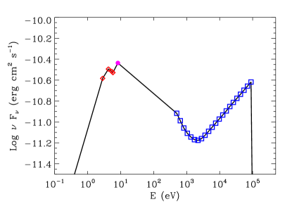
Figure 1: The spectral energy distribution for  1H0419-577 . Open diamonds are the fluxes from the OM optical and UV broad band filters discussed in the text; the filled circle is the continuum flux taken from the simultaneous  HST-COS observation; open squares are from the unabsorbed model for the X-ray continuum, obtained from the EPIC-pn observation.

We exploited the simultaneous  XMM-Newton and  HST-COS observation to constrain the SED of  source. The shape of the SED at lower energy is constrained by the  XMM-Newton OM and by  HST , while the  EPIC-pn camera covers the higher energy range. For this purpose we estimated the UV continuum of the source at 1500 Å in the complete  HST-COS spectrum. We selected a wavelength region not contaminated by any emission lines (1495 Å–1505 Å) and we took the average value of the 83 spectral points comprised in it.
We cut off the SED at low ($\rm E\leq 1.36\,eV$) and high energy ($\rm E\geq 100\,keV$). Indeed, the AGN spectral energy distribution falls off with the square of the energy above 100 keV while the optical-UV bump has an exponential cutoff in the infrared (Ferland et al. 2003). We show the SED in Fig. 1. From a numerical integration of the SED we calculated the source bolometric luminosity ($\rm\log L_{\rm bol}=45.95$ erg s^-1): for the SMBH hosted in  1H0419-577 the Eddington ratio is therefore $L_{\rm bol}/L_{\rm Edd}=0.5$. The source ionizing luminosity in the 1-1000 Ry energy range is $\rm\log L_{\rm ion}=45.43$ erg s^-1.

4 Spectral analysis

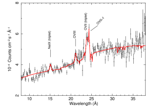
Figure 2: Composite RGS spectrum of  1H0419-577, rebinned for clarity. The solid line corresponds to the best fit model. The main emission features are labeled.

4.1 RGS continuum fitting

We show the composite RGS spectrum of  1H0419-577 in Fig. 2. We fitted the spectrum in the 8-38  Å band and we applied a factor 5 binning. Because the (more appropriate) C-statistic cannot be computed in the case of our combined fluxed spectrum, for the fit we used the $\chi^{2}$ statistic. We checked that at least 20 counts were collected in each spectral bin, as required for using the $\chi^{2}$ statistic. We took into account the cosmological redshift and the effects of Galactic neutral absorption; we used the HOT model (collisional ionized plasma) in SPEX for it, considering a column density of   $N{\rm{}_{H}}$ =$1.26\times 10^{20}$ cm^-2 (Kalberla et al. 2005) along the line of sight and a temperature of 0.5 eV to mimic a neutral gas.
We modeled the continuum emission with a broken power law. The best fit parameters we obtained for it are $\Gamma_{1}=2.73\pm 0.02$ and $\Gamma_{2}=2.30\pm 0.03$ as indexes, with a break energy of $\rm E_{0}=0.80\pm 0.03\,keV$.

4.2 RGS emission lines

Superposed on the underlying continuum the spectrum exhibits emission lines, most of which are broadened. To model the broad emission features of the spectrum, we added to the fit a Gaussian for each candidate emission line, leaving the centroid, the line-width and the flux as free parameters. We also tested the significance of the improvement of the  $\chi^{2}_{\nu}$ given by the extra component through an F-test. The F-test is trustworthy in testing the presence of an emission line if the line normalization is allowed to vary also in the negative range (Protassov et al. 2002).
We show the results in Table 2. Three broad components gave a highly significant improvement of the fit. Beside the Ne ix blended triplet, and the O viii  Ly$\rm{\,\sc{\alpha}}$ line, respectively redshifted at $\approx$ 15.1 Å and $\approx$ 21.2 Å (Fig. 2), the most prominent broad emission feature we were able to detect in the spectrum is a blend of the lines of the O vii triplets. In Fig. 3 we provide a zoom on the 20-26 Å spectral region where O vii and O viii lines are seen. To fit the spectrum in this complex region, we first modeled the prominent narrow line visible at $\approx$ 24.4 Å with a delta function, finding a rest wavelength of $22.11\pm{0.08}$ Å for it. Therefore, we could identify this line as due to the forbidden transition of  O vii : the line is formally detected with the F-test giving a significance above 99.99%. The line was unresolved, but we could however estimate un upper limit for its line-width. Assuming $\approx$ a 3:1 for the forbidden-to-intercombination line ratio (Porquet & Dubau 2000), we provided the intercombination and resonance lines corresponding to the detected O vii-f line. After adding these two narrow lines, the spectrum was still poorly fitted in the the 23.5-24.5 Å, showing broad prominent residuals. Hence, we added to the fit a broad-line leaving the centroid free to vary in the range among the known transitions of the O VII triplets. The modeling of the oxygen emission features allows a proper detection of any intervening absorption system (e.g Costantini et al. 2007). Indeed, in the same wavelength region covered by the blend of the O vii lines, transitions from O iv-O vii are in principle present.
Beside the O vii-f line, we determined upper limits for the luminosity of several other narrow lines. Since the narrow line width is not resolved in the RGS spectrum, we modeled them with a delta function. We estimated the upper limits by adding to the fit a delta line at the wavelength of the known transition, and fitting the maximum normalization where the line is undetectable over the continuum. The parameters of the X-ray narrow lines are listed in the upper panel of Table 4.

Figure 3: Middle Panel: best fit to the RGS spectrum of  1H0419-577 in the 20-26 Å wavelength range. Upper Panel: absorbing components. The neutral absorbers at z=0 and the local warm absorber (shifted downward for plotting purpose) are displayed as solid lines. Lower Panel: profiles of the broad and narrow emission features

Table 2: Parameters of 1H0419-577 X-ray broad lines.

Ion	Rest wavelength	$\log(L_{\rm obs})$	FWHM	F-test
	Å	erg s-1	km s-1
O vii	$21.69\pm{0.07}$	$42.44\pm 0.07$	$11000\pm{1000}$	$>99.99\%$
O viii	$19.17\pm{0.06}$	$41.95\pm 0.16$	$5000\pm{2000}$	99.2%
Ne ix	$13.66\pm{0.05}$	$41.81\pm 0.15$	$5000\pm{3000}$	99.6%

4.3 RGS absorption lines

We modeled the X-ray absorbing gas of  1H0419-577 using the photoionized-absorption model XABS in SPEX. This model calculates the transmission of a slab of material, where all ionic column densities are linked through the ionization balance. Thus, it computes the whole set of absorption lines produced by a photoionized absorbing-gas, for a gas column density   $N{\rm{}_{H}}$  and an ionization parameter $\xi$. The gas outflow velocity $v_{\rm out}$ is another free parameter. We kept instead the RMS velocity broadening of the gas frozen to the default value (100 km s^-1). The input ionization balance for XABS is sensitive to the spectral shape of ionizing SED: we calculated it running the tool  xabsinput, with the SED described in Sect. 3 as input. The  xabsinput routine, makes internally use of the Cloudy code (ver.10.00, Ferland et al. 1998) to determine the ionization balance. In the calculation we assume solar abundances as given in Cloudy (see Cloudy manual for details). We found that the absorption features of  1H0419-577 can be fitted by a thin and lowly-ionized absorber. The best fit parameters are   $N{\rm{}_{H}}$ =$8\pm 3\times 10^{19}$ cm^-2and $\log\xi=0.03\pm 0.15$. We had no strong constraints on a possible outflow velocity. We estimated an upper limit at 99% confidence ($\Delta\chi^{2}$=6.67 for one parameter) of $v_{\rm out}\leq 210$ km s^-1. By adding the absorption component we achieved an improvement of the statistic of $\Delta\chi^{2}$=25. According to the F-test, given the 3 extra degrees of freedom, this $\chi^{2}$ improvement is significant at a 99.7% level of confidence. The most prominent absorption lines (Fig. 3) are transitions from lowly ionized oxygen species such as O iv and O v, respectively redshifted to 25.1  Å and 24.7  Å (Fig. 3). In Table 6 we provide the column densities of the main ions of the absorber, provided by XABS. As a comparison, we fitted also each ionic column density individually with the SLAB model. SLAB is a simpler absorption model where all the ionic column densities are modeled independently, since they are not linked each other by any photoionization model. In the line-by-line fit with SLAB, we kept the same outflow velocity and velocity broadening of the previous XABS fit. XABS predictions and SLAB fit are consistent within the quoted errors. Therefore, hereafter we will use the value provided by XABS as reference.

Table 3: Column densities of the main absorbing ions for  1H0419-577 .

	XABS	SLAB
Ion	$\rm\log(N_{ion})$	$\rm\log(N_{ion})$
	cm-2	cm-2
O iv	$16.2\pm{0.1}$	$16.1\pm 0.2$
O v	$16.2\pm{0.1}$	$16.4\pm 0.4$
O vi	$15.9\pm{0.1}$	$\leq\,15.6$
O vii	$15.2\pm{0.1}$	$15.9\pm 0.5$
C v	$16.1\pm{0.1}$	$\leq\,16.8$
N iv	$15.3\pm{0.1}$	$\leq 15$
N v	$15.3\pm{0.1}$	$15.4_{-1.7}^{+0.4}$
N vi	$15.3\pm{0.1}$	$\leq 15.5$

4.4 The UV and optical narrow emission lines

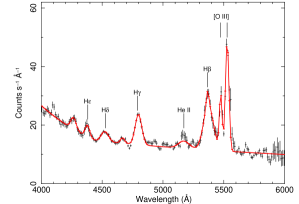
Figure 4: OM optical grism spectrum of  1H0419-577 in the 4000-6000 Å range. The best fit model is displayed by a solid line. The main emission features from the hydrogen Balmer series an the [O iii] doublet are labeled.

Table 4: Parameters of the X-ray, UV, and optical narrow lines of  1H0419-577 .

Ion	Wavelength	$\log(L_{\rm obs})$	FWHM
	Å	erg s-1	km s-1
C vi	33.73	$\leq 41.67$	…
N vi	29.53	$\leq 40.73$	…
N vii	24.78	$\leq 40.65$	…
O vii-f	$22.11\pm{0.08}$	$41.84\pm 0.08$	$\leq 2500$
O viii	18.97	$\leq 41.69$	…
Ne ix	13.70	$\leq 40.52$	…
C iv	1551	42.89	$805\pm 40$
C iv	1548	43.03	$805\pm 40$
Ly$\rm{\,\sc{\alpha}}$	1215	43.18	$488\pm 24$
O vi	1038	42.69	$840\pm 42$
O vi	1032	42.73	$840\pm 42$
$[{O\textsc{iii}}]$	5007	$43.13\pm 0.01$	$1200\pm 100$
$[{O\textsc{iii}}]$	4959	$42.71\pm 0.03$	$500\pm 300$
H${\beta}$	4861	$42.14\pm 0.12$	488 (fixed)

We studied also the narrow emission-lines present both in the optical and in the UV spectrum. In the middle panel of Table 4, we list the UV narrow emission -lines derived from the fit performed on the simultaneous HST-COS spectrum. Each line was fitted by a combination of resolved broad and narrow components (see Sect. 3.1 and Fig. 2 in E11 for details). From the parameters of the fit, a formal 5% error was estimated on the narrow component, both for the line luminosity and for the line width. This error does not include any uncertainty associated to the blend of the narrow and the broad components.
Finally, in the lower panel of Table 4 we list the optical narrow emission-lines, obtained by fitting the OM grism spectrum (Fig. 4). We fitted the continuum with a broken power-law, and we modeled the sinusoidal feature due to a residual Modulo-8 fixed pattern noise with Gaussians. We clearly detected the broadened features of the hydrogen Balmer series (H${\beta}\,\rm\lambda 4861$ Å, H${\gamma}\,\rm\lambda 4341$ Å, H${\delta}\,\rm\lambda 4102$ Å and H${\epsilon}\,\rm\lambda 3970$ Å) and the narrow emission lines of the [O iii] doublets $\rm\lambda\lambda$5007,4959   Å. In the analysis we used the luminosities of the [O iii] lines and of the narrow component of H${\beta}$. We modeled the [O iii] lines with Gaussian profiles, leaving the centroid, the line-width and the flux as free free parameter. The full width at half maximum (FWHM) of the [O iii] lines was resolved and it is reported in Table 4. In fitting the H${\beta}$ line, we used two Gaussians, respectively for a narrow and a broad component. We set the wavelength of the narrow component to the nominal wavelength of the H${\beta}$ transition and its width to the one of the  Ly$\rm{\,\sc{\alpha}}$ narrow component measured in the UV, leaving only the normalization as free paramaters. All the parameters of the broad component were instead left free. The fitted  FWHM for the broad H$\beta$ component ($4700\pm 400$ km s^-1) is within the range of the three broad components of  Ly$\rm{\,\sc{\alpha}}$ measured in the UV spectrum ($\approx$ 1000, 3400 and 14 000 km s^-1).

5 Photoionization modeling

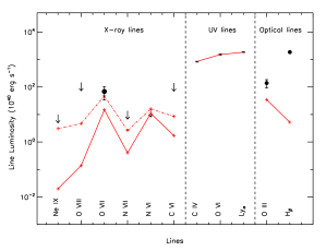
Figure 5: Best fit of the intrinsic luminosities of the UV narrow emission lines (middle panel). The model is displayed by a solid line only to guide the eye. The line luminosities predicted by the model in the X-ray (left panel) and in the optical (right panel) band are displayed by red crosses connected by a solid line. The model agrees with the upper limits for the X-ray lines, but does not fit the optical lines. The qualitative best fit model for the X-ray lines is also shown by red crosses connected by a dot dashed line. Error bars, when larger than the size of the plotting symbols, are also shown. Note that a 3$\sigma$ error bar is shown for O VII-f line.

Table 5: Covering factor, column density and ionization parameter for the gas emitting the UV and X-ray narrow lines in  1H0419-577 .

	$C_{v}$	$\rm\log\hbox{ $N{\rm{}_{H}}$ }$	$\rm\log\xi$
		cm-2
UV	$0.104\pm 0.006$	$21.67\pm 0.25$	$0.48\pm 0.15$
X	0.104 (fixed)	$21.40\pm 0.25$	$1.44\pm 0.15$

To estimate the global properties of the gas emitting the narrow lines in  1H0419-577, we used the photoionization code Cloudy v. 10.0 (Ferland et al. 1998). In the calculation we assumed total coverage of the source and a gas density of $\rm 10^{8}\,cm^{-3}$. We note that the assumption on the gas density is not critical for the resulting gas parameters. Indeed line ratios of He-like ions are not sensitive to the gas density over a wide range of density values (Porquet & Dubau 2000). We used the SED described in Sect. 3 and the ionizing luminosity derived from it as input. We created a grid of line luminosities for a wide range of possible gas parameters: the column density ranged between $\rm\log\hbox{ $N{\rm{}_{H}}$ }=[19-23]\,cm^{-2}$, and the ionization parameter between $\rm\log\xi=[-0.3-2.7]\,erg\,cm\,s^{-1}$, with a spacing of 0.25 dex and 0.15 dex respectively. In the fitting routine, we first computed for each grid entry the gas covering factor $C_{v}$, by imposing to the model match the luminosity of the  Ly$\rm{\,\sc{\alpha}}$ line. Hence, we modeled the data by minimizing the merit function:

$$\chi^{2}=\sum\frac{(C_{v}L_{c}-L_{\rm obs})^{2}}{\sigma_{\rm obs}^{2}},$$

where $L_{c}$ is the model-predicted luminosity of each line, $C_{v}$ is the gas covering factor and $L_{\rm obs}$ is the observed line luminosity, with statistical error $\sigma_{\rm obs}$. We fitted all the UV, X-ray and optical luminosities listed in Table 4. The C iv, O vi and [O iii] doublets were considered as a blend and $3\sigma$ upper limits for the X-ray lines of Table 4 were also included.
A model with a $\approx$ 10% covering factor $\rm\log\hbox{ $N{\rm{}_{H}}$ }\approx 21.67$ cm^-2and $\log\xi\approx 0.48$ fits the three UV data points (Ly$\rm{\,\sc{\alpha}}$, C iv, O vi) and agrees with all the upper limits for the X-ray luminosities. In fitting the UV lines we obtain a minimum $\chi^{2}/\rm{d.o.f}=0.35/1$. With just one degree of freedom the probability of getting such a low observed $\chi^{2}$ or lower for a correct model is 0.45.The derived parameter for the UV emitter are outlined in Table 8. We report the width of the grid step as error on the parameters. The error for the covering factor is estimated propagating the error ($\approx$5%) on the luminosity of the  Ly$\rm{\,\sc{\alpha}}$ line.
This best fit model neither match the luminosity of the O vii-f nor the luminosities of the optical lines, suggesting that X-ray and optical lines arise in a gas with different physical conditions. It was not possible to estimate the parameters of the X-ray emitter through a proper fit, because we had only one line detection. However, the measured upper limits provide useful constraints for the model. Assuming the same covering factor of the UV emitter, we selected in the grid all the models in agreement with the measured upper limits and matching the luminosity of the O vii-f line within 3$\sigma_{\rm obs}$. In this calculation, we added the contribution of the best-fit UV model to the X-ray luminosities. We find that the selected models have $\log\hbox{ $N{\rm{}_{H}}$ }$ ($[21.13-21.93]$ cm^-2) and their ionization parameter is comprised within $\log\xi=[1.12-2.06]$. Therefore, the fit which best model the O vii-f line has a column density consistent, within a grid step, with the UV emitter one ($\log\hbox{ $N{\rm{}_{H}}$ }\approx$21.40 cm^-2) but has a higher ionization parameter ($\log\xi\approx$1.44). This may indicate a geometrical connection between the UV and the X-ray emitter. In the case when also the gas covering factor is left free, we obtained a larger parameter range, ($C_{v}=[0.03-0.60]$, $\log\hbox{ $N{\rm{}_{H}}$ }=[20.90-23.00]$ cm^-2), still indicating a higher ionization parameter ($\log\xi=[1.12-1.60]$) with respect to the UV-emitter. We remark also that none of the models in our grid match the optical-lines luminosities. Finally we note that models with parameters consistent with the warm absorber detected in the RGS spectrum neither fit the UV ($\chi^{2}=[246-631]$) nor the the X-ray (the O vii-f is not fitted within $\approx 6\sigma$) emission lines. We show the best fit models for the UV and the X-ray emission lines in Fig. 5. The derived parameter for the X-ray emitter are outlined in the second row of Table 8.

6 Comparison between the UV and the X-ray absorber

We investigate the possible relationship between the UV absorber found for  1H0419-577 in E11 and the X-ray absorber found here (Sect. 4.3) by comparing the gas parameters independently measured in the two different wavebands.
Three different outflow components ($\rm v_{1}=-38\,\hbox{km s${}^{-1}$}$, $\rm v_{2}=-156\,\hbox{km s${}^{-1}$}$ and $\rm v_{3}=-220\,\hbox{km s${}^{-1}$}$) were identified in the UV. Because of the the lower RGS resolution, we were not able to resolve any of the UV components; however our upper limit for the outflow velocity of the X-ray absorber is consistent with all of them. Thus, it is likely that in the X-rays we observed a blended superposition of the UV components.
In Table 6 we compared of the UV and X-ray column densities for C ii,  C iv,  N v,  O vi. Absorption lines from O vi were detected in both bands, while lines from C ii, C iv and N v were detected only in the UV; however their column densities could be predicted by our XABS model. We report in Table 6 the sum of the column densities of the kinetic components 1, 2 and 3, obtained using a UV partial covering model, with a power law distribution of the optical depth (see E11 for details). The column densities found independently in the X-ray and in the UV agree within the quoted errors for all ions.
The ionization parameter of the UV absorber is given in terms of ${U_{H}=\frac{Q_{H}}{4\pi R^{2}c\hbox{ $N{\rm{}_{H}}$ }}}$ ( where $Q_{H}$ is the rate of hydrogen ionizing photons emitted by the source, $R$ is the absorber distance from the source, c is the speed of light, and   $N{\rm{}_{H}}$  is the total hydrogen column density) rather than in terms of $\xi$. For the SED of  1H0419-577, $\log\xi=1.7+\log U_{H}$. In the UV the determination of $U_{H}$ is not well constrained: for a broken power-law SED and for a gas with solar abundances $\log U_{H}$ =[-1.7 to -1.5] (Fig. 8 in E11). Applying the conversion factor just given this value corresponds to $\rm\log\xi$ =[0 to 0.2], consistent with the more constrained value found here for the X-ray absorber: $\rm\log\xi$ =[-0.12 to 0.18].

Table 6: Comparison between the UV and X-ray column densities of the absorbing ions in  1H0419-577 .

	UV	X
Ion	$\rm\log(N_{ion})$	$\rm\log(N_{ion})$
	cm-2	cm-2
C ii	$12.99-13.08$	13.11
C iv	$15.16-15.29$	15.42
N v	$15.16-15.31$	15.36
O vi	$15.83-15.96$	15.89

7 Discussion

7.1 Absorber distance and energetics

The spectral analysis of the RGS spectrum of 1H0419-577, together with the analysis of the simultaneous COS spectrum (E11) revealed that the X-ray and the UV emission spectra of  1H0419-577 are both absorbed by a thin, weakly ionized absorber. As pointed out in Sect. 6 the ionization parameter and the ionic column densities measured independently in the UV and in the X-ray agree with each other. Thus, it is likely that the UV and X-ray warm absorber are one and the same gas. In the UV the kinetic structure of the warm absorber is resolved, with three outflowing components detected. The bulk of absorbing column density is carried by the components 2+3 (see Table 1 and 2 and Fig. 3 in E11). Therefore in the lower resolution X-ray spectrum we likely detected a blend of the UV kinetic components dominated by the UV components 2+3. Having established the connection between the UV and the X-ray absorber, we can exploit the complementary information derived in the two wavebands to estimate the warm absorber location and energetics.
In the following discussion we consider that an ionized medium, parameterized by $\rm\log\xi\approx 0.03$ and $N{\rm{}_{H}}$ $\approx 8\times 10^{19}$ cm^-2(this paper), is outflowing from the source at the velocity of the UV component 3 ($\rm v_{3}=-220\,\hbox{km s${}^{-1}$}$). Additionally, we use a a gas number density $n_{\rm H}\leq\,25\,\rm cm^{-3}$, as estimated in E11 for the UV component 2+3. This upper limit for the gas number density was derived from the ratio of the (non detected) first excited metastable and the ground level of C ii. As already pointed out in Sect. 6, the C ii column density measured in the UV is well accounted for by our absorber model. We note however that in the COS spectrum, the C ii 1334.5 Å profile is possibly asymmetric, and the centroid is slightly shifted with respect to the UV component 3: at least part of the C II emission may in principle arise in a kinetic component separated from the UV component 3. However, this possible additional component is not evident in any other lines.
Given the X-ray UV connection just established, the following discussion is based on the assumption that the upper limit for the gas density estimated in the UV may be applied to the UV/X-ray absorber. We assume a thin shell geometry for the outflow. In this approximation, the outflow is spherically shaped, with a global covering factor of the line of sight $C_{g}$. Each outflowing shell, $\Delta r$ thick, is partially filled with gas, with a volume filling factor $f$. The volume filling factor $f$ can be estimated analytically (Blustin et al. 2005), from the condition that the kinetic momentum of the outflow must be of the order of the momentum of the absorbed radiation plus the momentum of the scattered radiation. Applying this condition, we found that the absorber in  1H0419-577 has a volume filling factor $f\approx\rm 3\times 10^{-3}$, suggesting that it may consist of filaments or fragments very diluted in the available volume and intercepting our line of sight.
Exploiting the tighter constraint on the ionization parameter provided by the present analysis we confirm the distance estimation given in E11:

$$R\geq(\frac{L_{\rm ion}}{n_{\rm H}\xi})^{1/2}\ga 3\,\rm kpc.$$ (1)

This estimation places the warm absorber at the host galaxy scale, well outside the central region with the broad-line region ($R_{\rm BLR}\approx 0.07\rm\,pc$, Turner et al. 2009). UV absorbers located at a galactic-scale distance are not uncommon in low-redshift quasars (see table 6 in E11 and references therein). The X-ray/UV connection we infer for this source would therefore make its low-$\xi$ absorber the first galactic scale X-ray absorber ever detected. A possible confining medium for an X-ray absorbers located at a $\approx$kpc from the nucleus could be a radio jet-like emission. This source is radio quiet, but a 843 MHz flux detection (Mauch et al. 2003) may be due to a weak radio lobe. More accurate radio measurements are required to test this possibility. Such a galactic-scale wind may be both AGN or starburst driven. However, for this source, the UV analysis suggests that the photoionization of the outflow may be dominated by the AGN emission (see discussion in E11 and references therein).
We estimated also an upper limit for the WA distance from the condition that the thickness $\Delta r$ of the outflowing-gas column should not overcome its distance $R$ from the centre (Blustin et al. 2005). Analytically, this condition is:

$$\frac{\Delta r}{R}\approx\frac{\hbox{ $N{\rm{}_{H}}$ }}{fn_{H}R}=\frac{\xi R\hbox{ $N{\rm{}_{H}}$ }}{L_{\rm ion}f}\leq 1.$$ (2)

From Eq. 2 we derived: $R\la 15\rm\,kpc$. We note that this distance is well within the typical extension of a galactic halo (e.g as mapped by H I emission for a large sample, de Blok et al. 2008). Therefore we use this estimation in the following to derive hard upper limits for the mass outflow rate and kinetic luminosity.
The outflow mass rate is given by

$$\dot{M}_{\rm out}=4\pi\mu m_{P}Rv\hbox{ $N{\rm{}_{H}}$ }C_{g}=[4-16]\,\hbox{{$M_{\odot}$ yr${}^{-1}$}},$$ (3)

where $\mu$=1.4 is the mean atomic mass per proton, $m_{P}$ is the proton mass. We assumed a covering factor $C_{g}$=0.5, given by the fact that outflows are seen in about 50% of the observed Seyfert galaxies (Dunn et al. 2007).
This value may be compared with the classical mass accretion rate of a black hole in the Eddington regime ($\dot{M}_{\rm Edd}=L_{\rm bol}/\eta c^{2}$) to obtain an estimation of the impact of the mass loss due to the outflow on the AGN. Assuming a typical accretion efficiency $\eta=0.1$ and taking $L_{\rm bol}=9\times 10^{45}\hbox{erg s${}^{-1}$}$, as estimated from the SED (see Sect. 3) we obtained

$$\dot{M}_{\rm Edd}\approx 2\hbox{{$M_{\odot}$ yr${}^{-1}$}}.$$ (4)

As found in most cases (see Costantini 2010), the mass outflow rate can be of the same order of the mass accretion rate, suggesting a balance between accretion and ejection in this system. The kinetic luminosity of the outflow is:

$$L_{\rm kin}=\frac{\dot{M}_{\rm out}v^{2}}{2}\approx 10^{40.7-41.4}\,\hbox{erg s${}^{-1}$},$$ (5)

and it represents a small fraction ($\la 10^{-2}$% ) of the AGN bolometric luminosity $L_{\rm bol}$; thus the outflow is not energetically significant in the AGN feedback scenario, where kinetic luminosities of a few percent of the bolometric luminosities are required (Scannapieco & Oh 2004). We finally estimated the maximum kinetic energy that the outflow can release into the interstellar medium, in the case it is steady all over the AGN life time ($\approx 4\times 10^{8}\rm\,yr$, Ebrero et al. 2009):

$$E_{\rm tot}\approx 10^{56.8-57.5}\,\rm erg.$$ (6)

As argued in Krongold et al. (2010) this value may in principle be sufficient to evaporate the interstellar environment out of the host galaxy. However, it is not trivial to couple this energy effectively to the galaxy (e.g. King 2010).

7.2 The origin of the emission lines

The simultaneous  HST-COS and  XMM-Newton observation of  1H0419-577 provided a set of narrow lines, ranging from the optical to the X-ray domain, suitable for photoionization modeling. We show that a single gas model cannot account simultaneously for all the narrow-lines emission. The UV lines are emitted by moderately ionized gas, intercepting about the 10% of the total AGN radiation field. This value for the covering factor is consistent with what previously reported ($C_{v}$=1.9%–20.5%, Baskin & Laor 2005). The X-ray lines are instead emitted in a more highly ionized gas phase: ($\log\xi\approx 1.44$). We also found that a gas with the same column density and covering factor as the UV emitter is a good description of the X-ray emission. This may suggest that the two emitters are two adjacent layers of the same gas.
Most of the optical emission is not accounted for by our model: it can explain only up to the 4% of the H${\beta}$ luminosity and the 0.3% of [O iii] luminosity. Lower densities are required to emit the [O iii] lines: the [O iii] $\lambda 5007$Å line is indeed collisionally de-excited for $n_{H}\ga 10^{5}\,\rm cm^{-3}$ (Osterbrock 1989). Our simple photoionization model cannot however account for the variety of gas physical conditions occurring in the narrow-line region. Our analysis suggests that the NLR is a stratified environment hosting a range of different gas components. Previous studies have shown that multi-component photoionization models are required for describing the narrow emission lines spectrum of AGN. The narrow line emission from the infrared to the UV is well reproduced assuming that the emitting region consists of clouds with a wide range of gas densities and ionization parameters (Ferguson et al. 1997). In the case of NGC 4151 more than one gas component, with different covering factor, are required to explain lines-emission even limiting the analysis to the soft X-ray regime (Armentrout et al. 2007). In the present case, the data quality did not allow us to test a more complex, multi-component scenario.
The estimated gas parameters of the warm absorber are largely inconsistent with the emitters. Thus, neither the UV nor the X-ray emitter can be regarded as the emission counter-part of the warm absorber. Therefore, a connection between the warm absorber and the gas in the NLR is discarded in the present case.

7.3 The geometry of the gas

The present analysis of the UV and X-ray spectrum of  1H0419-577 revealed three distinct gas phases: the UV/X-ray warm absorber, the X-ray emitter ($\log\xi_{\rm X}\approx 1.44$) and the UV emitter ($\log\xi_{\rm UV}\approx 0.48$). We used the line width of Table 4 to estimate qualitatively the location of the emitters. Assuming that the NLR gas is moving in random keplerian orbits with an isotropic velocity distribution, the velocity $v_{FWHM}$ by which the narrow lines are broadened is given by (Netzer 1990):

$$v_{FWHM}=\sqrt{\frac{4GM}{3R}},$$ (7)

where $M$ is the mass of the SMBH and $R$ is the radial distance from it. The  FWHM of the UV lines ([488–805]  km s^-1 , Table 4) give therefore the approximate location of the UV emitter:

$$R^{\rm em}_{\rm UV}\approx[1-3]\rm\,pc.$$ (8)

This distance would imply a gas number density of $n_{H}=(L_{\rm ion}\xi_{UV})/(R^{\rm em}_{\rm UV})^{2}\approx 10^{7-8}\,\rm cm^{-3}$ at the location of the UV emitter, consistent with the range of gas density and distance where these lines are optimally emitted (Ferguson et al. 1997). The X-ray emitter is consistent to be a gas with covering factor and column density similar to the UV emitter. This suggests that it may be a layer of gas adjacent to UV emitter. The higher X-ray ionization parameter may by produced both by a smaller distance to the SMBH and by a lower gas density. The gas density in the NLR ionization cone has a smoothly decreasing radial profile (Bianchi et al. 2006). Therefore, if the UV and X-ray emitter are not radially detached, as we suggested, a similar gas density for both the emitters can be assumed. From the definition of ionization parameter, it follows that:

$$R^{\rm em}_{\rm X}\approx\sqrt{\frac{\xi_{\rm UV}}{\xi_{\rm X}}}R^{\rm em}_{\rm UV}\approx[0.3-1.0]\,\rm pc.$$

This estimation is consistent with the lower limit for the distance ($R^{\rm em}_{\rm X}\ga 0.1\rm\,pc$) implied by the upper limit for the broadening of the O vii-f line. This first order estimation places the emitters on a very different distance scale compared to the absorber, again arguing against a connection between emission and absorption in this source. We did not detect the NLR in absorption: this may indicate that the NLR ionization cone is not along our line of sight, as this would produce visible O vii absorption lines. We are possibly detecting scattered light from the NLR. The presence of a circumnuclear scattering region has been proposed, for example, for the case of NGC 4151 (Kraemer et al. 2001).

8 Summary and conclusions

We analyzed and modeled the X-ray, UV and optical data of the Seyfert 1.5 galaxy  1H0419-577. Simultaneous X-ray (RGS) and UV (HST-COS) spectra of the source were taken, to study the absorbing-emitting photoionized gas in this source. Optical data from the OM were also used for the present analysis. We found three distinct gas phases with different ionization.

The X-ray and the UV spectrum are both absorbed by the same, lowly ionized warm absorber ($\log\xi=0.03\pm 0.15$). The outflow is likely to be located in the host galaxy, at a distance $R\ga 4\,\rm kpc$ from the central source. The kinetic luminosity of the outflow is small fraction ($\la 10^{-2}$%) of the AGN bolometric luminosity, making the outflow unimportant for the AGN feedback. However, such a galactic-scale X-ray absorber, like the one we serendipitously discovered in this source, might still play a role in the host galaxy evolution.

We performed photoionization modeling of the narrow lines emitter using the available UV, X-ray and optical narrow emission lines. The analysis indicates that the narrow-lines emitters are not the emission counter-part of the WA. A connection between the WA and the NLR can therefore be discarded in this case.

The X-ray emission lines are emitted in a more highly ionized gas phase compared to the one producing the UV lines. We suggest a geometrical connection between the UV and the X-ray emitter, where the emission takes place in a single gas layer, located at $\approx$ pc scale distance from the center. In this scenario, the X-ray lines are emitted in a portion of the layer located closer to the SMBH.

Finally, our analysis suggests that the NLR is a stratified environment, hosting a range of gas phases with different ionization and density.