Direct coupling information measure from non-uniform embedding

Abstract

A measure to estimate the direct and directional coupling in multivariate time series is proposed. The measure is an extension of a recently published measure of conditional Mutual Information from Mixed Embedding (MIME) for bivariate time series. In the proposed measure of Partial MIME (PMIME), the embedding is on all observed variables, and it is optimized in explaining the response variable. It is shown that PMIME detects correctly direct coupling, and outperforms the (linear) conditional Granger causality and the partial transfer entropy. We demonstrate that PMIME does not rely on significance test and embedding parameters, and the number of observed variables has no effect on its statistical accuracy, it may only slow the computations. The importance of these points is shown in simulations and in an application to epileptic multi-channel scalp EEG.

I Introduction

In the recent years the study of causality in multivariate time series, has gained much attention, also due to the advances of complex networks from time series, and has contributed in the understanding of complex systems (Zanin et al., 2012). Considering the global system as a network, the interest in this work is in the direct effect a driving sub-system, observed through a variable $X$, may have on the evolution of a response sub-system, observed through a variable $Y$. This is to be distinguished from an indirect effect $X$ may have on $Y$ via other sub-systems, say $Z$, where the observed variables in $Z$ are referred to as confounding variables.

There are established linear measures of direct causality, such as the conditional Granger Causality index (CGCI) (Geweke, 1984). Though many nonlinear directional coupling measures have been proposed in the last decade Hlaváčková-Schindler et al. (2007), there are only few extensions accounting for indirect effects, such as the partial phase synchronization (Schelter et al., 2006a) and the partial transfer entropy (PTE) (Vakorin et al., 2009; Papana et al., 2012). A possible reason for this unbalanced production of measures might be the increased data requirements when adding confounding variables in the calculations. For example, for the same delay embedding with embedding dimension $m$ (and delay $\tau$) for $X$ and $Y$, the transfer entropy (TE) measuring the causal effect from $X$ to $Y$ requires the estimation of a joint probability distribution of dimension $2m+1$ ($m$ for $X$, $m$ for $Y$ and 1 for the future of $Y$). Extending TE to PTE when totally $K$ variables are observed, the dimension becomes $Km+1$, and eventually PTE fails for a large $m$ or $K$. This is indeed a common practical setting, e.g. electroencephalograms (EEG), climatic records, and stock portfolio, and there have been some suggestions on reducing the dimension (Shibuya et al., 2011; Marinazzo et al., 2012; Runge et al., 2012a).

Dimensionality reduction is the first drawback we intend to successfully address with the proposed measure. The next drawback is related to the embedding parameters $m$ and $\tau$. In real settings, one does not know aforehand the best choice of embedding parameters, and recent works have shown that the measure performance is very much dependent on them Papana et al. (2011). The third drawback is the need for a statistical test of significance, which for nonlinear measures is computationally intensive requiring resampling test using surrogate data.

We recently proposed a non-uniform embedding scheme, bypassing the problem of selecting the embedding parameters, and derived a measure for bivariate directional coupling, the conditional Mutual Information from Mixed Embedding (MIME) Vlachos and Kugiumtzis (2010). For this we used information criteria and found that the $k$-nearest neighbors (kNN) estimate of entropies, and consequently mutual information (MI), is stable and efficient, as it adapts the local neighborhood to the dimension of the state space (Kraskov et al., 2004) (for a similar approach based on entropy and binning estimate see Faes et al. (2011)). Here, we extend the measure MIME to multivariate time series, and form the partial MIME (PMIME) that can detect direct coupling. The idea is first to reconstruct a point (vector) in the subspace of the joint state space of lagged variables $X$, $Y$ and $Z$, derived from the non-uniform embedding scheme with the purpose of explaining best the evolution of $Y$. The derived mixed embedding vector contains only the most relevant components from all variables, avoiding thus large dimension that would deteriorate the estimation. The presence of components of $X$ in this vector indicates that $X$ has some effect on the evolution of $Y$ and then the derived information measure PMIME is positive, whereas the absence indicates no effect and then PMIME is exactly zero.

We explain the measure in detail in Section  II. In Section III, we demonstrate the effectiveness of PMIME, compared also to PTE and CGCI, on a number of simulated systems and a multi-channel scalp EEG recording. We conclude in Section IV.

II The measure of partial mutual information from mixed embedding

Let $\{x_{t},y_{t},z_{1,t},\ldots,z_{K-2,t}\}_{t=1}^{n}$ be a multivariate time series of $K$ variables $X,Y,Z_{1},\ldots,Z_{K-2}$, and we want to estimate the effect of $X$ on $Y$ conditioning on $Z\!=\!\{Z_{1},\ldots,Z_{K-2}\}$. The future of $Y$ at each time step $t$ is generally represented by a vector of $T$ feature values, $\mathbf{y}_{t}^{T}\!=\![y_{t+1},\ldots,y_{t+T}]$. This is an extension of the one step ahead, $\mathbf{y}_{t}^{1}\!=\!y_{t+1}$, and can be more appropriate in some settings, e.g. a relatively dense sampling for continuous-timed systems. The lags of $X$, $Y$ and $Z$ are searched within a range given by a maximum lag for each variable, e.g. $L_{x}$ for $X$ and $L_{y}$ for $Y$. When all variables are of the same type, e.g. EEG signals, it is natural to assume the same maximum lag $L$ for all variables. Let us denote the set of all lagged variables at time $t$ as $W_{t}$, containing the components $x_{t},x_{t-1},\ldots,x_{t-L_{x}}$ of $X$ and the same for the other variables.

We use an iterative scheme to form the mixed embedding vector $\mathbf{w}_{t}\in W_{t}$ starting with an empty embedding vector, $\mathbf{w}_{t}^{0}\!=\!\emptyset$ Vlachos and Kugiumtzis (2010). In the first iteration, termed first embedding cycle, we find the component in $W_{t}$ being most correlated to $\mathbf{y}_{t}^{T}$ given by the kNN estimate of MI, $w_{t}^{1}\!=\!\mbox{argmax}_{w\in W_{t}}I(\mathbf{y}_{t}^{T};w)$, and we have $\mathbf{w}_{t}^{1}\!=\![w_{t}^{1}]$. In the second embedding cycle, the mixed embedding vector is augmented by the component $w_{t}^{2}$ of $W_{t}$, giving most information about $\mathbf{y}_{t}^{T}$ additionally to the information already contained in $w_{t}^{1}$, i.e. $w_{t}^{2}\!=\!\mbox{argmax}_{w\in W_{t}}I(\mathbf{y}_{t}^{T};w|w_{t}^{1})$, where the conditional mutual information (CMI) is again estimated by kNN, and the mixed embedding vector is $\mathbf{w}_{t}^{2}\!=\![w_{t}^{1},w_{t}^{2}]$. The progressive vector building stops at the embedding cycle $j$ and we have $\mathbf{w}_{t}\!=\!\mathbf{w}_{t}^{j-1}$, if the additional information of $w_{t}^{j}$ selected at the embedding cycle $j$ is not large enough. In Vlachos and Kugiumtzis (2010), we quantified this with the termination criterion

$$I\big{(}\mathbf{y}_{t}^{T};\mathbf{w}_{t}^{j-1}\big{)}/I\big{(}\mathbf{y}_{t}^{T};\mathbf{w}_{t}^{j}\big{)}>A$$ (1)

for a threshold $A<1$.

The obtained mixed embedding vector $\mathbf{w}_{t}$ may contain any of the lagged variables $X,Y,Z_{1},\ldots,Z_{K-2}$, and the interest in terms of the causality $X\!\rightarrow\!Y$ is whether there are any components of $X$ in $\mathbf{w}_{t}$. Let us denote the components of $X$ in $\mathbf{w}_{t}$ as $\mathbf{w}_{t}^{x}$, for $Y$ as $\mathbf{w}_{t}^{y}$ and for the other variables in $Z$ as $\mathbf{w}_{t}^{z}$. To quantify the causal effect of $X$ on $Y$ conditioned on the other variables in $Z$, we define PMIME as

$$R_{X\!\rightarrow\!Y|Z}\!=\!{I(\mathbf{y}_{t}^{T};\mathbf{w}_{t}^{x}\mid\mathbf{w}^{y},\mathbf{w}^{z})\over I(\mathbf{y}_{t}^{T};\mathbf{w}_{t})}.$$ (2)

The numerator is the CMI of the future response vector and the part of the mixed embedding vector formed by lags of the driving variable, accounting for the rest part of the vector. The form of CMI is similar to PTE, but in PTE the uniform delay embedding vectors of $X$, $Y$ and $Z$ are used and the delay parameters have to be set. The normalization in eq.(2) with the MI of the future response vector and the whole mixed embedding vector restricts $R_{X\!\rightarrow\!Y|Z}$ in [0,1], and it is zero if there are no driving components in the mixed embedding vector ($\mathbf{w}_{t}^{x}\!=\!\emptyset$), meaning there is no direct causal effect from $X$ on $Y$, and it is one if the mixed embedding vector is totally dominated by the driving variable ($\mathbf{w}_{t}^{y}\!=\!\mathbf{w}_{t}^{z}\!=\!\emptyset$). The latter is rather unlikely to be met in practice and in general we expect $R_{X\!\rightarrow\!Y|Z}$ to be closer to zero than to one.

The free parameters in PMIME are the maximum time lags for each variable, e.g. $L_{X}$, the time horizon $T$ in the future response vector $\mathbf{y}_{t}^{T}$ and the threshold $A$ in the termination criterion. The selection of maximum lags is not critical and can be arbitrarily large at the cost of excessive computations. A rule of thump is to have a small number of lags for maps (discontinuous series of observations), and a larger number of lags for flows (smoothly changing observations), which for oscillating time series should cover one or more oscillation periods Kugiumtzis (1996). The time horizon $T$ is also dependent on the underlying dynamics. Nevertheless $T\!=\!1$ is widely used in works on linear and nonlinear causality measures, but we have argued that $T>1$ may be more appropriate in cases of densely sampled time series Vlachos and Kugiumtzis (2010).

The threshold $A$ is the only inherent parameter of PMIME. For MIME, it was found after a simulation study that $A\!=\!0.95$ is an appropriate choice to avoid false positives, i.e. components of $X$ entering $\mathbf{w}_{t}$ in the absence of coupling. We extend this study here and compare the fixed threshold $A$ to an adjusted threshold for the significance of $I(\mathbf{y}_{t}^{T};w_{t}^{j}|\mathbf{w}_{t}^{j-1})$, the CMI for the selected component $w_{t}^{j}$ at the embedding cycle $j$. As the null distribution for the null hypothesis H₀: $I(\mathbf{y}_{t}^{T};w_{t}^{j}|\mathbf{w}_{t}^{j-1})\!=\!0$, is not known, we form it empirically by shuffling randomly the components of the vector $w_{t}^{j}$ and the rows of the matrix $\mathbf{w}_{t}^{j-1}$. This random shuffling scheme aims at obtaining the most independent joint distribution that gives largest bias in the estimation of CMI, setting higher significance threshold and thus making the termination criterion more stringent. Then if the original $I(\mathbf{y}_{t}^{T};w_{t}^{j}|\mathbf{w}_{t}^{j-1})$ is larger than the $(1-\alpha)\%$ percentile of the ensemble of the randomized $I(\mathbf{y}_{t}^{T};w_{t}^{j}|\mathbf{w}_{t}^{j-1})$, we accept $w_{t}^{j}$ as significant and proceed to the next embedding cycle, otherwise the mixed embedding scheme terminates and $\mathbf{w}_{t}\!=\!\mathbf{w}_{t}^{j-1}$.

We found that the adjusted threshold criterion is more adaptive than the fixed threshold to system complexity, time series length and noise level. For illustration, we consider the system of $K$ coupled Hénon maps, defined as

$$\begin{array}[]{ll}x_{i,t}=1.4-x_{i,t-1}^{2}+0.3x_{i,t-2},&\mbox{for}\,\,i=1,K\\ x_{i,t}=1.4-0.5C(x_{i-1,t-1}+x_{i+1,t-1})+(1-C)x_{i,t-1}^{2}+0.3x_{i,t-2},&\mbox{for}\,\,j=2,\ldots,K-1\end{array}$$ (3)

where $C$ is the coupling strength. For the example of $K\!=\!3$, it is shown in Table 1 that for weak coupling ($C\!=\!0.1$), $A\!=\!0.95$ is too conservative and a larger $A$, such as 0.97 or even better 0.99, is needed to include components of the driving variable in the mixed embedding vector for the two true direct couplings.

$X_{1}\!\rightarrow\!X_{2}$ $X_{3}\!\rightarrow\!X_{2}$ $X_{2}\!\rightarrow\!X_{1}$ noise-free $A\!=\!0.95$ 1 2 0 $A\!=\!0.97$ 41 25 0 $A\!=\!0.99$ 72 70 3 $\alpha\!=\!0.01$ 21 11 0 $\alpha\!=\!0.05$ 51 35 0 $\alpha\!=\!0.1$ 59 47 0 20$\%$ noise $A\!=\!0.95$ 22 11 0 $A\!=\!0.97$ 59 46 5 $A\!=\!0.99$ 79 92 36 $\alpha\!=\!0.01$ 20 4 0 $\alpha\!=\!0.05$ 48 37 3 $\alpha\!=\!0.1$ 63 57 8

Table 1: Number of times PMIME is positive for 100 realizations of three coupled Hénon maps ($C\!=\!0.1$) with true coupling $X_{1}\!\rightarrow\!X_{2}$ and $X_{3}\!\rightarrow\!X_{2}$, and false coupling $X_{2}\!\rightarrow\!X_{1}$. The parameters are $n\!=\!512$, $L\!=\!5$, $T\!=\!1$, and the stopping criterion is set by a fixed threshold $A$ and an adjusted threshold determined by $\alpha$.

However, in the presence of noise (observational Gaussian white noise with standard deviation (SD) 20% of the data SD), a larger $A$ allows for components of non-driving variables entering the mixed embedding vector, giving small false direct couplings. The choice of $A$ should balance these two effects and it seems that in practice a fixed threshold cannot be optimized. On the other hand, the adjusted threshold seems to work well for both noise-free and noisy time series, and the choice of $\alpha\!=\!0.05$ balances well sensitivity, i.e. probability of having positive PMIME for true direct couplings, and specificity, i.e. probability of having zero PMIME when there is no direct coupling.

III Simulation Study

Next we compare PMIME (with the adjusted threshold at $\alpha\!=\!0.05$) to the conditional Granger causality index (CGCI) (Geweke, 1984), and the partial transfer entropy (PTE) (Vakorin et al., 2009; Papana et al., 2012), respectively. We report the best obtained results for CGCI and PTE optimizing the parameter $m$ for the model order in CGCI and the embedding dimension in PTE. To assess statistically the sensitivity and specificity of the measures we compute the measures on 100 realizations from each system. PMIME is considered significant if it is positive, whereas the significance of CGCI and PTE is determined by the surrogate data test (for the null hypothesis of no coupling) using time-shifted surrogates at a significance level $\alpha=0.05$ Quian Quiroga et al. (2002).

Before we show detailed results on a number of linear stochastic, nonlinear stochastic and chaotic systems, we demonstrate the superiority of PMIME in terms of sensitivity and specificity on the system of $K$ coupled Hénon maps. As shown for $K\!=\!5$ in Fig. 1a, for the true direct coupling $X_{3}\!\rightarrow\!X_{2}$ PMIME increases more than the other measures with the coupling strength $C$ and up to $C\!=\!0.8$. The larger increase of PMIME with $C$, particularly for small $C$, is justified by the statistical significance of the measures (Fig. 1b). On the other hand, for the indirect coupling $X_{4}\!\rightarrow\!X_{2}$, PMIME is zero for all $C$ (a slight deviation is observed only for very large $C$), whereas PTE increases slowly with $C$ and CGCI fluctuates at some positive level (Fig. 1c), both tending to be more significant with the increase of $C$ (Fig. 1d).

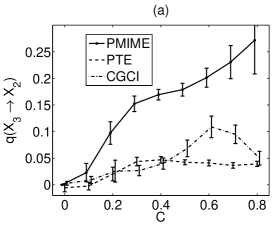
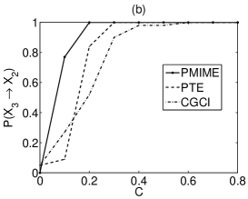
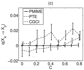
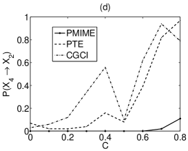
Figure 1: Estimated coupling $q$, where $q$ is any of PMIME, PTE and CGCI given in the legend, as a function of coupling strength $C$ for the system of $K\!=\!5$ coupled Hénon maps: (a) $X_{3}\!\rightarrow\!X_{2}$, and (c) $X_{4}\!\rightarrow\!X_{2}$. The parameters are $n\!=\!1024$, $T\!=\!1$ for all measures, $m\!=\!2$ for PTE and CGCI. Each error bar denotes the mean and SD over 100 realizations, and the error bars are slightly displaced horizontally for better visualization. The panels in (b) and (d) show the estimated probability $P$ of detecting the coupling in (a) and (c), respectively, which is the relative frequency PTE and CGCI found significant at the significance level $\alpha\!=\!0.05$ using 100 time-shifted surrogates, or the relative frequency of PMIME being positive.

$K\!=\!5$ $K\!=\!15$ $K\!=\!25$ $X_{(K-1)/2}\!\rightarrow\!X_{(K-1)/2+1}$ PMIME 0.105(1.00) 0.063(0.92) 0.061(0.79) PTE 0.021(0.89) 0.001(0.15) 0.000(0.10) CGCI 0.040(0.85) 0.188(0.68) 0.230(0.67) $X_{(K-1)/2}\!\rightarrow\!X_{(K-1)/2+2}$ PMIME 0.000(0.00) 0.000(0.01) 0.001(0.02) PTE -0.005(0.04) 0.001(0.02) 0.000(0.07) CGCI 0.009(0.15) 0.064(0.44) 0.136(0.45)

Table 2: Mean of coupling measure and relative frequency for its statistical significance in parentheses from 100 realizations of coupled Hénon maps ($C\!=\!0.2$) with varying number of variables $K$. Results are shown for the true direct coupling (first block) and the indirect coupling (second block) of the variables in the center part of the chain of the $K$ variables. The parameter setup is as for Fig. 1.

A challenging situation is when the number of variables $K$ increases. We observed that even for the optimal $m$, PTE looses significance in detecting the true direct coupling, and CGCI tends to falsely detect direct coupling, whereas PMIME attains both high sensitivity and specificity, decreasing rather slowly with the increase of $K$. These features get more pronounced for the most interacting variables and as $K$ gets large, as shown in Table 2 for the variables in the middle of the chain of the coupled Hénon maps. We note that regardless of $K$ the mixed embedding vector for PMIME contains always few components, one (more seldom two) of which are from the driving variable in the presence of causal effect.

In the following, further results for the performance of PMIME and comparison to PTE and CGCI are presented for multivariate time series from different discrete and continuous systems and for different time series lengths and levels of noise added to the time series.

III.1 Linear multivariate stochastic process - 1

The first system is a linear vector autoregressive process of order 5 in 4 variables, VAR${}_{4}(5)$ (model 1 in Winterhalder et al. (2005))

$$\begin{array}[]{l}x_{1,t}=0.8x_{1,t-1}+0.65x_{2,t-4}+e_{1,t}\\ x_{2,t}=0.6x_{2,t-1}+0.6x_{4,t-5}+e_{2,t}\\ x_{3,t}=0.5x_{3,t-3}-0.6x_{1,t-1}+0.4x_{2,t-4}+e_{3,t}\\ x_{4,t}=1.2x_{4,t-1}-0.7x_{4,t-2}+e_{4,t}\end{array}$$

where $e_{i,t}$, $i=1,\ldots,4$, are white noise components having zero mean and unit covariance matrix. The true direct causality connections are $X_{1}\rightarrow X_{3}$, $X_{2}\rightarrow X_{1}$, $X_{2}\rightarrow X_{3}$, and $X_{4}\rightarrow X_{2}$.

For all discrete systems we use $T=1$, and for PMIME $L=5$, which here matches the larger lag in the process. For PTE and CGCI we vary the embedding dimension and model order, respectively, $m=2,\ldots,5$, in order to investigate for the best $m$ and show also the dependence of their performance on the parameter $m$. The results from 100 Monte Carlo realizations of the system VAR${}_{4}(5)$ are shown in Table 3.

PMIME PTE($m=2$) PTE($m=3$) PTE($m=4$) PTE($m=5$) CGCI($m=2$) CGCI($m=5$) $X_{2}\rightarrow X_{1}$ 0.348(1.00) 0.034(0.53) 0.073(1.00) 0.116(1.00) 0.115(1.00) 0.175(1.00) 0.750(1.00) $X_{1}\rightarrow X_{3}$ 0.610(1.00) 0.160(1.00) 0.158(1.00) 0.134(1.00) 0.093(1.00) 0.608(1.00) 0.587(1.00) $X_{2}\rightarrow X_{3}$ 0.073(0.99) 0.007(0.07) 0.013(0.25) 0.015(0.18) 0.015(0.09) 0.046(1.00) 0.361(1.00) $X_{4}\rightarrow X_{2}$ 0.487(1.00) 0.048(0.78) 0.049(0.80) 0.081(0.99) 0.126(1.00) 0.089(1.00) 0.622(1.00) $X_{1}\rightarrow X_{2}$ 0.002(0.09) 0.010(0.03) 0.013(0.11) 0.013(0.11) 0.013(0.14) 0.007(0.13) 0.010(0.08) $X_{3}\rightarrow X_{1}$ 0.000(0.02) 0.015(0.06) 0.012(0.07) 0.010(0.07) 0.011(0.05) 0.011(0.28) 0.010(0.07) $X_{1}\rightarrow X_{4}$ 0.003(0.11) 0.007(0.01) 0.012(0.05) 0.015(0.11) 0.017(0.20) 0.004(0.05) 0.010(0.03) $X_{4}\rightarrow X_{1}$ 0.000(0.03) 0.012(0.03) 0.013(0.02) 0.012(0.02) 0.013(0.03) 0.008(0.23) 0.010(0.07) $X_{3}\rightarrow X_{2}$ 0.001(0.03) 0.009(0.05) 0.013(0.10) 0.013(0.09) 0.014(0.06) 0.006(0.07) 0.010(0.07) $X_{2}\rightarrow X_{4}$ 0.002(0.04) 0.010(0.04) 0.013(0.05) 0.018(0.06) 0.021(0.09) 0.004(0.03) 0.010(0.06) $X_{3}\rightarrow X_{4}$ 0.001(0.04) 0.005(0.04) 0.011(0.08) 0.015(0.10) 0.019(0.10) 0.004(0.03) 0.010(0.03) $X_{4}\rightarrow X_{3}$ 0.000(0.00) 0.001(0.07) 0.004(0.01) 0.008(0.07) 0.011(0.06) 0.003(0.10) 0.010(0.03)

Table 3: Mean of coupling measure and relative frequency for its statistical significance in parentheses from 100 realizations of the system VAR${}_{4}(5)$ and $n=512$. For PTE the results are shown for $m=2,\ldots,5$ and for CGCI for $m=2,5$. The true direct couplings are shown in a frame box.

PMIME is high and always positive for the four direct couplings and essentially zero for the other couplings. The largest frequency of false positive PMIME is for $X_{1}\rightarrow X_{4}$ (11 in 100 realizations), but still the PMIME values are very small (the mean is 0.003). Regarding the true direct couplings, the weakest causal effect is estimated by PMIME for $X_{2}\rightarrow X_{3}$ (mean 0.073), but still PMIME is positive almost always (99 in 100 realizations). This true direct coupling cannot be estimated by PTE for any $m$, and the best rejection rate of H₀ of no causal effect is for $m=3$ (25 rejections in 100 significance randomization tests using time-shifted surrogates). However, the selection $m=3$ is not appropriate for $X_{4}\rightarrow X_{2}$, as it gives only 80 rejections, which is much less than the highest rejection rate of 100% obtained by PMIME and CGCI, and also by PTE for $m=5$. This example demonstrates how PMIME resolves the ambiguity in the selection of the appropriate embedding for PTE. The selection of a suitable order $m$ may be an issue also for the linear measure CGCI, as a small $m$ does not give good specificity (for two non-existing direct couplings the rejection rate is 23% and 28%) and sensitivity (though the power of the test is 1.0 for all four true direct couplings, the mean CGCI is much smaller for $m=2$ than for $m=5$ in three of the four couplings).

III.2 Linear multivariate stochastic process - 2

The second linear VAR process is of order 4 in 5 variables, VAR${}_{5}(4)$ (model 1 in Schelter et al. (2006b))

$$\begin{array}[]{l}x_{1,t}=0.4x_{1,t-1}-0.5x_{1,t-2}+0.4x_{5,t-1}+e_{1,t}\\ x_{2,t}=0.4x_{2,t-1}-0.3x_{1,t-4}+0.4x_{5,t-2}+e_{2,t}\\ x_{3,t}=0.5x_{3,t-1}-0.7x_{3,t-2}-0.3x_{5,t-3}+e_{3,t}\\ x_{4,t}=0.8x_{4,t-3}+0.4x_{1,t-2}+0.3x_{2,t-2}+e_{4,t}\\ x_{5,t}=0.7x_{5,t-1}-0.5x_{5,t-2}-0.4x_{4,t-1}+e_{5,t}\end{array}$$

The simulation setup is the same as for the first linear system, and the results are shown in Table 4.

PMIME PTE($m=2$) PTE($m=3$) PTE($m=4$) PTE($m=5$) CGCI($m=2$) CGCI($m=5$) $X_{1}\rightarrow X_{2}$ 0.224(1.00) 0.012(0.26) 0.010(0.22) 0.019(0.69) 0.017(0.61) 0.023(0.62) 0.108(1.00) $X_{1}\rightarrow X_{4}$ 0.196(1.00) 0.022(0.50) 0.016(0.56) 0.012(0.49) 0.010(0.27) 0.101(1.00) 0.208(1.00) $X_{5}\rightarrow X_{1}$ 0.411(1.00) 0.061(0.99) 0.044(1.00) 0.037(0.99) 0.032(0.96) 0.243(1.00) 0.225(1.00) $X_{2}\rightarrow X_{4}$ 0.110(0.95) 0.008(0.08) 0.009(0.24) 0.005(0.16) 0.005(0.11) 0.033(0.87) 0.119(1.00) $X_{5}\rightarrow X_{2}$ 0.400(1.00) 0.052(1.00) 0.036(0.95) 0.030(0.95) 0.026(0.85) 0.185(1.00) 0.194(1.00) $X_{5}\rightarrow X_{3}$ 0.171(1.00) 0.002(0.00) 0.011(0.39) 0.011(0.30) 0.009(0.26) 0.031(0.86) 0.092(1.00) $X_{4}\rightarrow X_{5}$ 0.494(1.00) 0.070(1.00) 0.048(1.00) 0.039(0.97) 0.032(0.93) 0.405(1.00) 0.320(1.00) $X_{2}\rightarrow X_{1}$ 0.017(0.22) 0.001(0.05) -0.001(0.05) -0.000(0.02) 0.000(0.04) 0.004(0.04) 0.010(0.07) $X_{1}\rightarrow X_{3}$ 0.007(0.13) 0.002(0.05) -0.001(0.04) -0.000(0.02) 0.000(0.03) 0.012(0.24) 0.010(0.04) $X_{3}\rightarrow X_{1}$ 0.013(0.13) -0.001(0.05) 0.000(0.03) -0.001(0.07) -0.000(0.05) 0.004(0.03) 0.008(0.04) $X_{4}\rightarrow X_{1}$ 0.009(0.12) -0.002(0.05) -0.002(0.04) -0.001(0.05) -0.000(0.03) 0.004(0.02) 0.010(0.08) $X_{1}\rightarrow X_{5}$ 0.014(0.16) -0.000(0.03) -0.001(0.06) 0.001(0.03) 0.002(0.07) 0.004(0.08) 0.010(0.04) $X_{2}\rightarrow X_{3}$ 0.004(0.10) 0.003(0.08) -0.001(0.05) 0.001(0.02) 0.000(0.05) 0.016(0.42) 0.010(0.03) $X_{3}\rightarrow X_{2}$ 0.009(0.13) -0.001(0.06) 0.001(0.08) 0.000(0.01) 0.000(0.05) 0.007(0.14) 0.010(0.04) $X_{4}\rightarrow X_{2}$ 0.009(0.15) -0.001(0.06) 0.000(0.02) 0.000(0.05) 0.001(0.03) 0.006(0.11) 0.010(0.02) $X_{2}\rightarrow X_{5}$ 0.009(0.12) 0.001(0.06) 0.000(0.05) 0.003(0.05) 0.002(0.01) 0.004(0.04) 0.011(0.06) $X_{3}\rightarrow X_{4}$ 0.004(0.12) 0.000(0.04) -0.002(0.05) -0.002(0.04) -0.000(0.03) 0.008(0.37) 0.010(0.03) $X_{4}\rightarrow X_{3}$ 0.005(0.07) 0.001(0.05) -0.001(0.05) -0.001(0.03) -0.001(0.04) 0.020(0.50) 0.009(0.06) $X_{3}\rightarrow X_{5}$ 0.013(0.17) -0.001(0.04) -0.001(0.05) 0.002(0.05) 0.001(0.02) 0.004(0.06) 0.011(0.01) $X_{5}\rightarrow X_{4}$ 0.007(0.15) 0.033(0.81) 0.004(0.10) 0.002(0.07) 0.004(0.11) 0.131(1.00) 0.011(0.05)

Table 4: Mean of coupling measure and relative frequency for its statistical significance in parentheses from 100 realizations of the system VAR${}_{5}(4)$ and $n=512$. For PTE the results are shown for $m=2,\ldots,5$ and for CGCI for $m=2,5$. The true direct couplings are shown in a frame box.

The results for VAR${}_{5}(4)$ are similar to these for the VAR${}_{4}(5)$. This example was included to show that for small time series from stochastic systems PMIME may be falsely positive at a rate higher than the nominal rate of $\alpha=0.05$. Here, the highest false positive rate was 22% for $X_{2}\rightarrow X_{1}$, but still PMIME was very small (in average one tenth of the weakest true direct coupling). On the other hand, PTE does not have overall high sensitivity and moreover there is no optimal $m$, e.g. for $X_{2}\rightarrow X_{4}$ the rejection rate is very small with highest rate being 24% for $m=3$, while for $X_{1}\rightarrow X_{2}$ the highest rejection rate is 69% for $m=4$. CGCI is again smaller for $m=2$ and the significance test has large size (higher false rejection rate than the nominal type I error of $\alpha=0.05$) and smaller power, which all improve with the increase of $m$.

Note that for the two linear stochastic processes, CGCI is the most appropriate measure of causality, but PMIME is comparable to CGCI.

III.3 Nonlinear multivariate stochastic process

Next we consider the nonlinear VAR process of order 1 in 3 variables, NLVAR${}_{3}(1)$ (model 7 in Gourévitch et al. (2006))

$$\begin{array}[]{l}x_{1,t}=3.4x_{1,t-1}(1-x_{1,t-1}^{2})\mbox{e}^{-x_{1,t-1}^{2}}+0.4e_{1,t}\\ x_{2,t}=3.4x_{2,t-1}(1-x_{2,t-1}^{2})\mbox{e}^{-x_{2,t-1}^{2}}+0.5x_{1,t-1}x_{2,t-1}+0.4e_{2,t}\\ x_{3,t}=3.4x_{3,t-1}(1-x_{3,t-1}^{2})\mbox{e}^{-x_{3,t-1}^{2}}+0.3x_{2,t-1}+0.5x_{1,t-1}^{2}+0.4e_{3,t}\end{array}$$

The simulation setup is the same as for the previous systems, and the results are shown in Table 5.

PMIME PTE($m=2$) PTE($m=3$) PTE($m=4$) PTE($m=5$) CGCI($m=2$) CGCI($m=5$) $X_{1}\rightarrow X_{2}$ 0.272(1.00) 0.056(0.98) 0.027(0.53) 0.020(0.39) 0.016(0.19) 0.006(0.08) 0.013(0.09) $X_{1}\rightarrow X_{3}$ 0.226(1.00) 0.045(0.86) 0.022(0.45) 0.016(0.26) 0.011(0.13) 0.005(0.07) 0.010(0.03) $X_{2}\rightarrow X_{3}$ 0.171(0.97) 0.033(0.71) 0.018(0.34) 0.015(0.27) 0.014(0.21) 0.090(1.00) 0.096(1.00) $X_{2}\rightarrow X_{1}$ 0.006(0.08) -0.006(0.04) -0.005(0.04) -0.004(0.04) -0.002(0.04) 0.004(0.04) 0.010(0.08) $X_{3}\rightarrow X_{1}$ 0.009(0.15) -0.008(0.01) -0.005(0.05) -0.003(0.04) -0.002(0.09) 0.004(0.00) 0.009(0.02) $X_{3}\rightarrow X_{2}$ 0.004(0.07) -0.009(0.04) -0.007(0.06) -0.002(0.05) 0.000(0.07) 0.004(0.07) 0.010(0.06)

Table 5: Mean of coupling measure and relative frequency for its statistical significance in parentheses from 100 realizations of the system NLVAR${}_{3}(1)$ and $n=512$. For PTE the results are shown for $m=2,\ldots,5$ and for CGCI for $m=2,5$. The true direct couplings are shown in a frame box.

Here again PMIME attains the best possible sensitivity (only for one true direct coupling there are three zero PMIME values) and good specificity (only for one false coupling the rate of positive PMIME values is well above the level of 5%, being 15%, and again the mean PMIME is almost two orders of magnitude smaller than for the true direct couplings). The largest lag in the process is one and therefore PTE looses sensitivity with the increase of $m$. For example, for $X_{2}\rightarrow X_{3}$ the rejection rate is 71% (already not high enough) for $m=2$, and drops with $m$ down to 21% for $m=5$. As expected, CGCI has very small sensitivity regardless of $m$, and can only identify one true direct coupling, the linear one $X_{2}\rightarrow X_{3}$.

III.4 Coupled Hénon maps

The system of $K$ coupled chaotic Hénon maps was previously defined in eq.(3). For $K\geq 3$, complete synchronization is not observed for any pair of variables as $C$ increases, but the time series of the driven variables explode for $C>1.0$ dependent on $K$, so $C$ is studied in the range $[0,0.8]$. Again 100 realizations for each system scenario are generated, for PTE and CGCI the free parameter is $m=2$ (embedding dimension and model order, respectively), for PMIME the standard parameter for maps $L=5$ is used, and for all measures the time ahead is $T=1$. Note that for this system, the choice $L=5$ is not suitable, as only lags up to 2 are present in the difference equations, whereas for PTE the parameter $m$ is optimal.

Some additional results to these shown earlier are shown below. First, the case of $K=3$ is presented for small time series of length $n=512$ and for the whole range of $C$. The true direct couplings are $X_{1}\rightarrow X_{2}$ and $X_{3}\rightarrow X_{2}$ and they are equivalent in strength. There is a symmetry in the coupling structure and therefore only three couplings are shown in Figure 2.

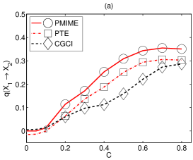
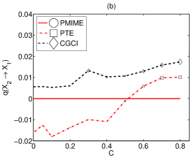
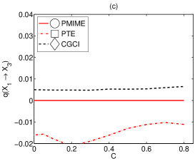
Figure 2: PMIME, PTE and CGCI measures (denoted collectively $q$) are given as functions of the coupling strength $C$ for the true direct causality $X_{1}\rightarrow X_{2}$ in (a), the non-existing couplings $X_{2}\rightarrow X_{1}$ in (b) and $X_{1}\rightarrow X_{3}$ in (c) for the coupled Hénon maps of $K=3$ and for time series length $n=512$. The number of rejections in 100 realizations of the randomization test determines the size of a symbol displayed for each measure and $C$, where in the legend the size of the symbols regards 100 rejections.

All measures confidently detect the true direct coupling for $C\geq 0.1$, but have very small power to detect it for $C=0.05$ and their average from 100 realizations is only slightly above the zero level (see Figure 2a). Note that the zero level for PTE is negative. This is better seen for the non-existing couplings in Figure 2b and c, while PMIME is always exactly zero. Moreover, for $X_{2}\rightarrow X_{1}$, PTE increases with $C$ and for larger $C$ it is found significant more often than the nominal level ($\alpha=0.05$), and the same holds for CGCI. The biased detection of false couplings with PTE (and CGCI) is more evident in the presence of noise, as shown in Figure 3, where white noise with SD being 20% of the data SD is added for each variable.

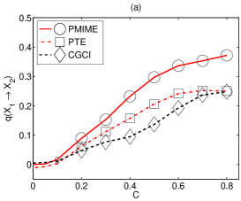
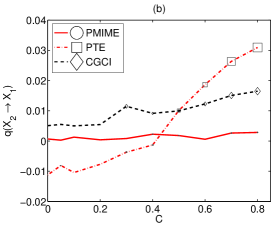
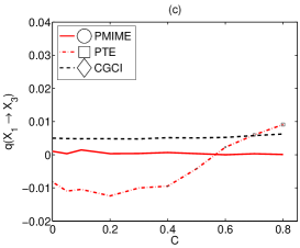
Figure 3: As Figure 2, but when white noise with SD 20% of the data SD is added.

Note that PMIME is not affected by noise and achieves the same power in detecting the true direct couplings, while it remains at the zero level when there is no direct coupling.

For $K=5$, the efficiency of PMIME as opposed to PTE and CGCI persists, as shown in the matrix plot of Figure 4 for all possible pairs.

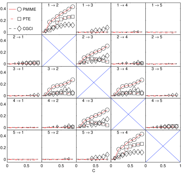
Figure 4: Matrix plot of all possible couplings of $K=5$ variables of the coupled Hénon maps ($n=1024$). Each panel regards a coupling of the variables with indices as shown at the top of the panel, and the organization of each panel is as for Figure 2.

The off-diagonal panels correspond to true direct couplings, the panels in column 1 and 5 correspond to non-existing coupling and all the other panels correspond to indirect couplings. PMIME estimates with high confidence the correct direct couplings for all $C\geq 1$. PTE is high and monotonically increasing only for the direct couplings $X_{1}\rightarrow X_{2}$ and $X_{5}\rightarrow X_{4}$, while for the other direct couplings it tends to decrease for $C>0.3$. It is pointed in Chicharro and Ledberg (2012) that PTE may not be monotonic to $C$ due to changes in the inter-dependence structure, but here PMIME does not seem to be affected. The interpretation of the PTE results as to the identification of the true direct couplings is difficult because small and significant PTE is observed both for true direct couplings and spurious couplings ($X_{2}\rightarrow X_{1}$ and $X_{4}\rightarrow X_{2}$). The same holds for CGCI, which is significant also for indirect couplings ($X_{1}\rightarrow X_{3}$ and $X_{5}\rightarrow X_{3}$).

About the same results are obtained when 20% white noise is added to the data, as shown in Figure 5.

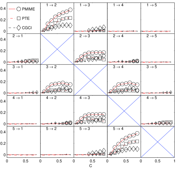
Figure 5: As Figure 4 but for 20% additive white noise.

PMIME is somehow smaller in magnitude but still can distinguish well the true direct couplings even for small $C$. On the other hand, PTE tends to be significant for more non-existing direct couplings than for the noise-free case ($X_{1}\rightarrow X_{3}$ and $X_{5}\rightarrow X_{3}$) following well CGCI to spurious detection of couplings.

In Table II, the performance of the measures PMIME, PTE and CGCI was shown for $K=5,15,25$, coupled Hénon maps. In Figure 6 more detailed results are shown.

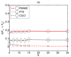
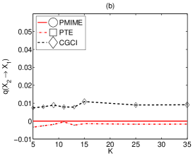
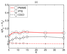
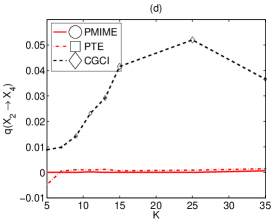
Figure 6: PMIME, PTE and CGCI measures (denoted collectively $q$) are given as functions of the number of variables $K$ of the coupled Hénon maps for time series length $n=1024$. (a) True direct causality $X_{1}\rightarrow X_{2}$. (b) Non-existing coupling $X_{2}\rightarrow X_{1}$. (c) True direct causality $X_{2}\rightarrow X_{3}$. (d) True indirect causality $X_{2}\rightarrow X_{4}$. The number of rejections in 100 realizations of the randomization test determines the size of a symbol displayed for each measure and $C$, where in the legend the size of the symbols regards 100 rejections.

For the two true direct couplings $X_{1}\rightarrow X_{2}$ and $X_{2}\rightarrow X_{3}$ for different $K$ in Figure 6a and c, respectively, PMIME is at the same significantly positive magnitude for as large $K$ as 35, an impressive result for a relatively small time series of length $n=1024$. The same holds for CGCI, which for the second coupling is smaller for smaller $K$, possibly due to the additional causal effect of other neighboring variables. On the other hand, PTE decreases both in magnitude and in statistical significance with $K$. In the case of the non-existing coupling $X_{2}\rightarrow X_{1}$ in Figure 6b, PMIME is always zero for any $K$, PTE is also statistically insignificant for any $K$, while CGCI is positive and statistically significant at about half of the 100 realizations. For the indirect causal connection $X_{2}\rightarrow X_{4}$ in Figure 6d, PMIME and PTE are again at the zero level and CGCI gets larger but less statistically significant. Thus CGCI is biased towards giving spurious direct causality, PTE cannot identify the direct causal effects, while PMIME attains optimal sensitivity and specificity.

The proper performance of PMIME persists also when noise is added to the time series, as shown for the same examples in Figure 7 in the presence of additional 20% white noise.

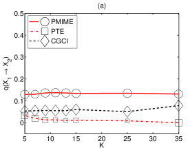
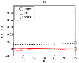
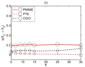
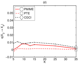
Figure 7: As Figure 6 but for 20% additive white noise.

CGCI and PTE exhibit the same shortcomings, and CGCI actually improves its specificity as it decreases in the case of indirect coupling. For the latter case, PMIME gets positive in a small percentage of the 100 realizations which is at the level of significance of the surrogate data test for the termination criterion.

III.5 Coupled Lorenz system

Next we study the system of three coupled identical Lorenz subsystems defined as

$$\begin{array}[]{l}\dot{x}_{1}=-10x_{1}+10y_{1}\\ \dot{y}_{1}=-x_{1}z_{1}+28x_{1}-y_{1}\\ \dot{z}_{1}=x_{1}y_{1}-8/3z_{1}\end{array}\quad\quad\begin{array}[]{l}\dot{x}_{i}=-10x_{i}+10y_{i}+C(x_{i-1}-x_{i})\\ \dot{y}_{i}=-x_{i}z_{i}+28x_{i}-y_{i}\\ \dot{z}_{i}=x_{i}y_{i}-8/3z_{i}\end{array}\quad i=2,3$$

The system of differential equations is solved using the explicit Runge-Kutta (4,5) method in Matlab and the time series are generated at a sampling time of 0.01 time units. The first variable of each subsystem is observed, denoted respectively as $X_{1}$, $X_{2}$ and $X_{3}$, and the direct couplings are $X_{1}\rightarrow X_{2}$ and $X_{2}\rightarrow X_{3}$. The same coupling strength $C$ is used for both couplings and for this setting it was assessed by observing the generated trajectories and characteristics of the observed time series (delay mutual information, correlation dimension and cross correlation) that complete synchronization is approached for $C>8$, so the measures were computed for $C=0,0.5,1,\ldots,8$. For each $C$, 100 realizations are generated, and we set $m=3$ for PTE and CGCI, $L=15$ for PMIME, and for both PMIME and PTE the future vector is formed for the time horizon $T=3$, i.e. $\mathbf{y}_{t}^{3}=[y_{t+1},y_{t+2},y_{t+3}]$ for the response variable $Y$, where $Y$ is any of the variables $X_{1}$, $X_{2}$ and $X_{3}$. The three steps ahead are chosen to represent better the time evolution of the continuous system, as suggested also in Vlachos and Kugiumtzis (2010). For CGCI, the option of a larger step ahead $T>1$ is not considered and it is computed for $T=1$.

The results of the simulations on noise-free time series of length $n=1024$ and $n=4096$ are shown in Figure 8, and when 20% white noise is added in Figure 9.

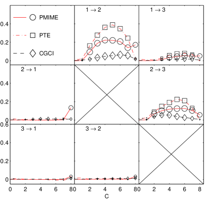
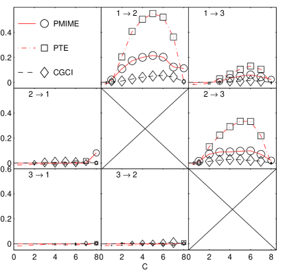
Figure 8: Matrix plot of all possible couplings of the Lorenz systems of $K=3$ subsystems and noise-free time series of length $n=1024$ on the left panel and $n=4096$ on the right panel. The organization of the panels is as for Figure 4.

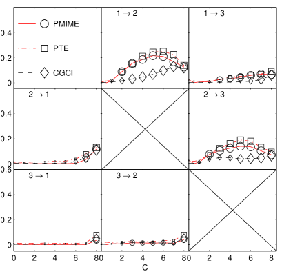
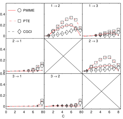
Figure 9: The same as Figures 8 but with 20% white noise added to the time series.

First, it is noted that the scale is not the same for the three measures and their magnitude is not a safe criterion of comparison. All three measures capture well the two true direct couplings for $C\geq 2$ with a rejection rate of the null hypothesis of no coupling at about 100%. For example, for noise-free data, $C=2$ and $n=1024$, the rejection rates for $X_{2}\rightarrow X_{3}$ are 99% for PMIME, 87% for PTE and 49% for CGCI, and change to 100% for all measures when $n=4096$. However, for weaker coupling with $C=1$ only PMIME detects confidently the true direct courplings, and for $X_{2}\rightarrow X_{3}$ it is 100% for $n=4096$ dropping to 23% for $n=1024$, whereas for PTE the respective rejection rates are 47% and 11%, while for CGCI are 64% and 13%. Thus though for stronger coupling all measures can detect well the direct true couplings, for smaller $C$ PMIME shows significantly better sensitivity. Regarding specificity, PMIME is also scoring best. For example, for the indirect coupling $X_{1}\rightarrow X_{3}$ and $C=2$, PMIME as well as CGCI give small rejection rate at the nominal significance level 5%, while PTE gives rejection rate 16% for $n=1024$ getting double for $n=4096$. For larger $C$, the rejection rate gets larger for all measures, indicating that for stronger coupling the indirect causal effects cannot be distinguished. For the cases of no coupling, all measures are at about the zero level, but only PMIME is statistically insignificant. For example for the non-existing coupling $X_{2}\rightarrow X_{1}$, the rejection rate of PTE is 16% for $n=1204$ and becomes double for $n=4096$, while for CGCI the respective rejection rates are much higher (87% and 97%), but PMIME gives no positive value for both $n$. PMIME has high rejection rates for $C=8$ because then the three variables are almost completely synchronized and the lagged variables may exhibit similar causal effects and thus the algorithm for mixed embedding does not systematically pick up a particular set of lagged variables.

The performance of the measures turns out to be persistent to the presence of noise (see Figure 9). PMIME tends to be biased towards detecting false direct couplings for small time series lengths ($n=1024$), but improves for larger time series lengths ($n=4096$). However, PTE and CGCI seem to suffer from lack of specificity for increasing $C$ also when $n$ increases.

Further investigation of the low specificity of PMIME for small $n$ indicated that this is merely due to the use of the adapted threshold for the termination criterion, i.e. the significance test for the conditional mutual information regarding the selected candidate lagged variable at a significance level $\alpha=0.05$. It seems that for this particular case (coupled Lorenz system, 20% noise), a fixed threshold of $A=0.97$ is more suitable, as shown in Figure 10 for $C=2$.

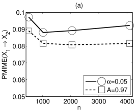
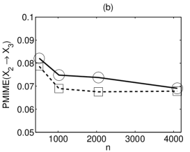
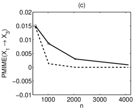
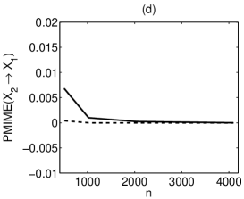
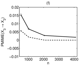
Figure 10: PMIME measure with adapted threshold ($\alpha=0.05$) and fixed threshold ($A=0.97$) are given as functions of the time series length $n$ for the true direct causality $X_{1}\rightarrow X_{2}$ in (a) and $X_{2}\rightarrow X_{3}$ in (b), the indirect causality $X_{1}\rightarrow X_{3}$ in (c), and the non-existing couplings $X_{2}\rightarrow X_{1}$ in (d), $X_{3}\rightarrow X_{1}$ in (e), and $X_{3}\rightarrow X_{2}$ in (f), for 3 Lorenz subsystems coupled with coupling strength $C=2$. The number of times in 100 realizations PMIME is positive determines the size of a symbol displayed for each threshold type and $n$, where in the legend of panel (a) the size of the symbols regards the maximum of 100 positive PMIME values.

For the two true direct couplings (Figure 10a and b) both threshold types give positive PMIME for all 100 realizations, but the adapted threshold gives larger PMIME values, which indicates that the termination criterion is less stringent and allows more components of the driving variable in the mixed embedding vector. This seems to have a negative consequence for the cases of indirect coupling $X_{1}\rightarrow X_{3}$ (Figure 10c) and the non-existing coupling $X_{3}\rightarrow X_{2}$ (Figure 10f), as the adapted threshold allows other than the lagged response variable components to enter in the mixed embedding vector, which results in positive PMIME more often than chance when $n$ is small. Nevertheless, this effect decreases with $n$. The use of the fixed threshold $A=0.97$ is more appropriate here as it does not produce this effect. However, as shown in Table 1 and suggested by other simulations not shown here, the fixed threshold does not adapt to different inter-dependence structures and data conditions. For example when 20% white noise is added to the system in Figure 10, the fixed threshold of $A=0.97$ gives still the highest specificity but has much lower sensitivity than the adapted threshold, e.g. for the weak coupling with $C=1$ and $n=4096$ the adapted threshold with $\alpha=0.05$ detects the true direct couplings (68 positive PMIME for $X_{1}\rightarrow X_{2}$ and 58 $X_{2}\rightarrow X_{3}$) and gives zero PMIME otherwise, while the fixed threshold $A=0.97$ gives zero PMIME also for the direct couplings.

III.6 Coupled Mackey-Glass system

The last simulated system is a continuous system of coupled identical Mackey-Glass delayed differential equations defined as

$$\dot{x}_{i}(t)=-0.1x_{i}(t)+\sum_{j=1}^{K}\frac{C_{ij}x_{j}(t-\Delta_{j})}{1+x_{j}(t-\Delta_{j})^{10}}\quad\mbox{for}\quad i=1,\ldots,K$$

For $K=2$ the system was first used in Senthilkumar et al. (2008) and then in Vlachos and Kugiumtzis (2010). The system is solved using the solver dde23 for delayed differential equations in Matlab and the time series are generated at a sampling time of 4 time units. For $K$ delayed differential equations $K$ time series are generated and the corresponding variables are denoted $X_{i}$, $i=1,\ldots,K$. When $\Delta_{j}=\Delta$, $j=1,\ldots,K$, the $K$ coupled subsystems are identical and we consider this case here. We also set $C_{ii}=0.2$ and let $C_{i,j}$ for $i\neq j$ determine the coupling structure.

For the future vector we set $\mathbf{y}_{t}^{3}=[y_{t+1},y_{t+\tau_{1}},y_{t+\tau_{2}}]$, where $\tau_{1}$ and $\tau_{2}$ are respectively the first minimum and maximum of the delayed mutual information for the response variable $Y$ (where $Y$ stands for any of $X_{i}$, $i=1,\ldots,K$). This choice is found in Vlachos and Kugiumtzis (2010) to better represent the short-term time evolution of the response system as the Mackey-Glass system exhibits irregular oscillations. This future vector is used in PMIME and PTE, while for CGCI the option of a larger step ahead $T>1$ is not considered and it is computed for $T=1$.

First we consider the case of $K=3$, $\Delta_{1}=\Delta_{2}=\Delta_{3}=20$, $C_{1,2}=C_{1,3}=C_{2,3}=C$ and $C_{2,1}=C_{3,1}=C_{3,2}=0$. The results of the three measures on 100 realizations of length $n=2048$ of this system for varying coupling strength $C$ are shown in Figure 11 for noise-free and noisy time series.

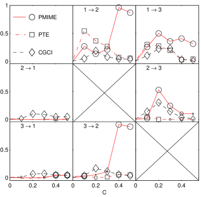
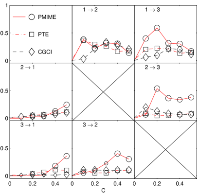
Figure 11: Matrix plot of all possible couplings of the $K=3$ coupled Mackey-Glass subsystems and noise-free time series of length $n=2048$ on the left panel, and with 20% additive white noise on the right panel. The organization of the panels is as for Figure 4.

For the noise-free data, PMIME detects best the three direct couplings (upper triangular panel components) and only for strong coupling $C\geq 0.4$ the number of positive values decreases for the coupling $X_{2}\rightarrow X_{3}$. The latter holds also for PTE, which is less sensitive for smaller coupling strengths, e.g. for $C=0.3$ and $X_{2}\rightarrow X_{3}$ PMIME gives 99 positive values and PTE only 34 statistically significant values. CGCI gives the highest sensitivity of 100% rejection rate of the null hypothesis of no-coupling, but this is of little benefit as it is followed by a very low specificity giving about the same highest rejection rate when there is no causal effect. PTE has also low specificity for all $C$, but PMIME only for $C\geq 0.4$. For example for the non-existing connection $X_{3}\rightarrow X_{2}$ and $C=0.3$, PTE gives 91 statistically significant values and PMIME 31 positive values, and these are 61 and 20, respectively for $C=0.2$, whereas CGCI gives constantly 100 statistically significant values.

For the noisy data, the sensitivity of the measures remain about the same, but the specificity gets lower for PTE and PMIME, with PMIME still performing better than PTE. For the setting $X_{3}\rightarrow X_{2}$ and $C=0.3$ the positive PMIME values are 63 and the statistically significant PTE values are 100, and the same holds for $C=0.2$ and the other two non-existing couplings.

For larger $K$ the differences of PMIME from PTE and CGCI become clearer. In Figure 12, the results are shown in the form of color maps for the statistical significance of the three measures for increasing number $K$ of weakly coupled Mackey-Glass subsystems.

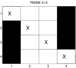
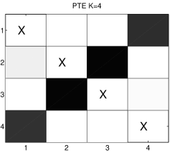
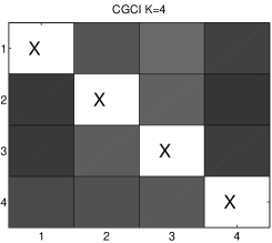
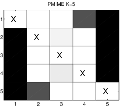
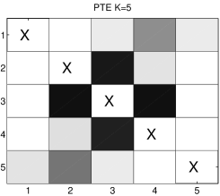
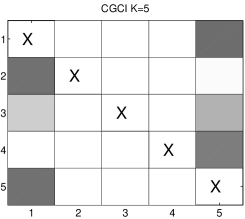
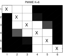
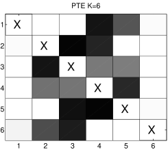
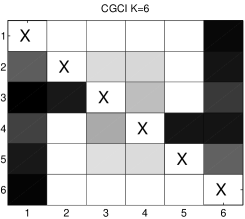
Figure 12: Color maps for the statistical significance of the three measures, PMIME in first column, PTE in the second column and CGCI in the third column, for all possible couplings of the $K$ coupled Mackey-Glass subsystems, where $K=4$ in the first row, $K=5$ in the second row and $K=6$ in the third row. The time series are noise-free and have length $n=2048$, and the subsystems have all the same delay $\Delta=20$ and each subsystem $X_{i}$ drives $X_{i-1}$ ($X_{i}\rightarrow X_{i-1}$) and $X_{i+1}$ ($X_{i}\rightarrow X_{i+1}$) with the same coupling strength $C$ ($X_{1}$ only drives $X_{2}$ and $X_{K}$ only drives $X_{K-1}$). The statistical significance of PMIME is given by the number of positive values in the 100 realizations and for PTE and CGCI by the number of rejections of the null hypothesis of no coupling. The gray color scale is from 0 (black) to 100 (white).

The variables (subsystems) have all the same delay $\Delta=20$ and each variable $X_{i}$ drives the variable next in the left ($X_{i}\rightarrow X_{i-1}$) and in the right ($X_{i}\rightarrow X_{i+1}$) with the same coupling strength $C$, where $X_{1}$ only drives $X_{2}$ and $X_{K}$ only drives $X_{K-1}$. The time series are noise-free and have length $n=2048$. An interesting feature of PMIME is that for any of $K=4,5,6$, there is no driving to the first variable $X_{1}$ and the last variable $X_{K}$, which are designed not to receive any causal effect from another variable, and the corresponding PMIME values are zero for all realizations. This is not preserved for the other two measures, with CGCI scoring close to PMIME with regard to driving of $X_{1}$ and $X_{K}$ for $K=6$. With further regard to specificity, PMIME gives positive values for the indirect couplings, but this inadequacy of PMIME improves with $K$ and for $K=6$ PMIME is zero for the most of the indirect couplings. The sensitivity of PMIME is the highest for all $K$ and PMIME is positive at all realizations (almost all for $K=5$) for all direct couplings. On the other hand, PTE and CGCI fail to detect the coupling structure of the system for any $K$ with PTE giving very low sensitivity and specificity.

We note here that the coupled Mackey-Glass system may involve complicated scenaria of coupling structures that are difficult to detect, and indeed PMIME gets also fooled and identifies spurious couplings. We observed this especially when the subsystems are not identical, setting different $\Delta_{i}$. For such situations, it remains an open problem whether the Granger causality measures can distinguish intrinsic dynamics from the inter-dependence structure, e.g. see the discussion in Sugihara et al. (2012). It should also be noted that the performance of PMIME could possibly be improved if we would choose a maximum lag $L>15$, e.g. in Vlachos and Kugiumtzis (2010) $L=50$ was used giving good results for $K=2$, but such large $L$ was not used here due to increased demand of computation time. However, for the simulations with $K>3$ we experienced that the computation of PTE with $m=5$ using 100 surrogates for the significance test is much more time demanding than for PMIME.

III.7 Real world example

Finally, we demonstrate the robustness of PMIME and its appropriateness in connectivity analysis and complex networks with an example of a human scalp multi-channel electroencephalogram (EEG) recording during an epileptic discharge (ED), i.e. an electrographic seizure of short duration . After artifact rejection, filtering and re-referencing, a set of 45 EEG signals were obtained and downsampled to 200 Hz frequency, covering 10 sec before and 10 sec after the start of an ED of duration 5.7 sec. We computed in each of the two periods PMIME, PTE and CGCI ($m\!=\!5$), all for $T\!=\!1$ and for all possible channel pairs on sliding windows of 2 sec with a step of 1 sec. To assess the strength of connectivity in the brain network estimated by each causality measure at each 2 sec window, we computed the average strength $S$ (mean of the measure values over all channel pairs). In an attempt to test the robustness of the causality measures to the network size, we repeated the same analysis 12 times on randomly selected subsets of the set of 45 channels. The results are shown in Fig. 13 for subset sizes 5, 15, 25 and 35.

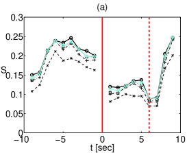
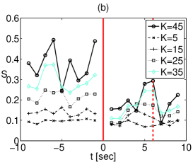
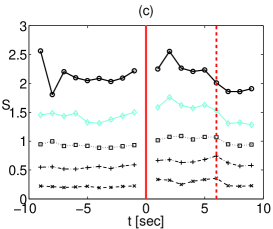
Figure 13: Mean average strength $S$ for PMIME in (a), PTE in (b) and CGCI in (c), on sliding windows along the period before and after the start of ED (marked with a vertical line at time zero) for the number of channels as shown in the legend. The vertical dashed line denotes the end of the ED.

We observe that only PMIME gives a stable pattern of connectivity strength over the two periods for any subset (some deviation can be seen for subset size 5). Moreover, PMIME distinguishes readily the period before ED, during ED and after ED. Similar results were obtained using the average degree, i.e. the mean binary connections obtained by the significance test for PTE and CGCI for $\alpha\!=\!0.05$ and when PMIME is positive.

IV Conclusions

The presented measure PMIME addresses successfully the problem of identifying direct causal effects in the presence of many variables. Intensive simulations on discrete- and continuous-timed coupled systems have confirmed this. While Taken’s embedding theorem advocates against the estimation of direct Granger causality in nonlinear systems Sugihara et al. (2012), and a vector with lagged components only from the response variable may be representing equivalently the mixed embedding vector, in practice PMIME pinpoints the set of the most and significantly contributing lagged components, identifying thus the direct causal effects.

PMIME does not rely on embedding parameters, and the structure of the mixed embedding vector allows for identification of the active lags of the driving variable affecting the response. The latter is currently an active research direction Runge et al. (2012b); Wibral et al. (2013), but we did not take it up in this study. Our initial results for detecting the true active lags in the bivariate analysis with MIME were promising, and work on this with PMIME is in progress.

We have improved the termination criterion in the progressive building of the mixed embedding vector, initially set for the bivariate measure MIME, and instead of using a fixed threshold we let the threshold be adjusted by the estimated bias using randomized replicates.

We have showed that PMIME scores highest in sensitivity and specificity as compared to PTE and CGCI, and moreover it does not require computationally intensive randomization (surrogate) significance test. While PMIME is much slower than PTE it is less computational intensive if PTE has to be combined with randomization test or when the number of observed variables gets large. The example on an EEG record of epileptic discharge demonstrates the usefulness of PMIME in analyzing multivariate time series from real complex systems and constructing causal networks.

References

- Zanin et al. (2012) M. Zanin, P. Sousa, D. Papo, R. Bajo, J. García-Prieto, F. Pozo, E. Menasalvas, and S. Boccaletti, Scientific Reports 2, 630 (2012).
- Geweke (1984) J. F. Geweke, Journal of the American Statistical Association 79, 907 (1984).
- Hlaváčková-Schindler et al. (2007) K. Hlaváčková-Schindler, M. Paluš, M. Vejmelka, and J. Bhattacharya, Physics Reports 441, 1 (2007).
- Schelter et al. (2006a) B. Schelter, M. Winterhalder, R. Dahlhaus, J. Kurths, and J. Timmer, Physical Review Letters 96, 208103 (2006a).
- Vakorin et al. (2009) V. A. Vakorin, O. A. Krakovska, and A. R. McIntosh, Journal of Neuroscience Methods 184, 152 (2009).
- Papana et al. (2012) A. Papana, D. Kugiumtzis, and P. G. Larsson, International Journal of Bifurcation and Chaos 22, 1250222 (2012).
- Shibuya et al. (2011) T. Shibuya, T. Harada, and Y. Kuniyoshi, Physical Review E 84, 061109 (2011).
- Marinazzo et al. (2012) D. Marinazzo, M. Pellicoro, and S. Stramaglia, Computational and Mathematical Methods in Medicine 2012 (2012).
- Runge et al. (2012a) J. Runge, J. Heitzig, V. Petoukhov, and J. Kurths, Physical Review Letters 108, 258701 (2012a).
- Papana et al. (2011) A. Papana, D. Kugiumtzis, and P. G. Larsson, Physical Review E 83, 036207 (2011).
- Vlachos and Kugiumtzis (2010) I. Vlachos and D. Kugiumtzis, Physical Review E 82, 016207 (2010).
- Kraskov et al. (2004) A. Kraskov, H. Stögbauer, and P. Grassberger, Physical Review E 69, 066138 (2004).
- Faes et al. (2011) L. Faes, G. Nollo, and A. Porta, Physical Review E 83, 051112 (2011).
- Kugiumtzis (1996) D. Kugiumtzis, Physica D 95, 13 (1996).
- Quian Quiroga et al. (2002) R. Quian Quiroga, A. Kraskov, T. Kreuz, and P. Grassberger, Physical Review E 65, 041903 (2002).
- Winterhalder et al. (2005) M. Winterhalder, B. Schelter, W. Hesse, K. Schwab, L. Leistritz, D. Klan, R. Bauer, J. Timmer, and H. Witte, Signal Processing 85, 2137 (2005).
- Schelter et al. (2006b) B. Schelter, M. Winterhalder, B. Hellwig, B. Guschlbauer, C. H. Lücking, and J. Timmer, Journal of Physiology-Paris 99, 37 (2006b).
- Gourévitch et al. (2006) B. Gourévitch, R. Bouquin-Jeannès, and G. Faucon, Biological Cybernetics 95, 349 (2006).
- Chicharro and Ledberg (2012) D. Chicharro and A. Ledberg, Physical Review E 86, 041901 (2012).
- Senthilkumar et al. (2008) D. V. Senthilkumar, M. Lakshmanan, and J. Kurths, Chaos: An Interdisciplinary Journal of Nonlinear Science 18, 023118 (2008).
- Sugihara et al. (2012) G. Sugihara, R. May, H. Ye, C. Hsieh, E. Deyle, M. Fogarty, and S. Munch, Science 338, 496 (2012).
- Note (1) The data were provided by V.K. Kimiskidis at the Department of Neurology III, Medical School, Aristotle University of Thessaloniki.
- Runge et al. (2012b) J. Runge, J. Heitzig, N. Marwan, and J. Kurths, Physical Review E 86, 061121 (2012b).
- Wibral et al. (2013) M. Wibral, N. Pampu, V. Priesemann, F. Siebenh hner, H. Seiwert, M. Lindner, J. T. Lizier, and R. Vicente, PLoS ONE 8, e55809 (2013).