Observation of modulation instability in a nonlinear magnetoinductive waveguide

Abstract

We report numerical and experimental investigations into modulation instability in a nonlinear magnetoinductive waveguide. By numerical simulation we find that modulation instability occurs in an electrical circuit model of a magnetoinductive waveguide with third-order nonlinearity. We fabricate the nonlinear magnetoinductive waveguide for microwaves using varactor-loaded split-ring resonators and observe the generation of modulation instability in the waveguide. The condition for generating modulation instability in the experiment roughly agrees with that in the numerical analysis.

I Introduction

Considerable effort has been devoted to controlling electromagnetic waves using metamaterials that consist of arrays of subwavelength structures. The macroscopic characteristics of metamaterials depend on the structure of the constitutive elements as well as the characteristics of the materials. It is therefore possible to design artificial media with extraordinary properties by devising the structure and material of the constitutive elements. Various kinds of unusual media and phenomena have been realized using metamaterials.Smith et al. (2004); Alitalo and Tretyakov (2009); Wang et al. (2009); Luk’yanchuk et al. (2010); Soukoulis and Wegener (2011); Zheludev and Kivshar (2012)

Efficient generation of nonlinear waves is a promising application of metamaterials.Pendry et al. (1999) When an electromagnetic wave is incident on a metamaterial composed of resonant elements such as split-ring resonators, the electromagnetic energy is compressed into a small volume at certain locations of the element at the resonant frequency. If nonlinear elements are placed at these locations, nonlinear phenomena occur efficiently. Several nonlinear phenomena such as harmonic generations,Klein et al. (2006); Shadrivov et al. (2008); Kim et al. (2008); Kanazawa et al. (2011); Nakanishi et al. (2012); Reinhold et al. (2012) bistability,Wang et al. (2008) and tunable mediaShadrivov et al. (2008); Wang et al. (2008); Powell et al. (2009) have been experimentally investigated.

In this paper, we focus on modulation instability. Modulation instabilities are observed in various nonlinear systems. In the field of optics, modulation instabilities in optical fibers have been actively investigated. When a continuous wave enters an optical fiber with third-order nonlinearity and the frequency of the incident wave is in the anomalous group velocity dispersion region of the fiber, the incident wave is converted to a pulse train. This phenomenon is referred to as (spontaneous) modulation instability.Agrawal (2006) The modulation instability has been intensively studied because it can be used to generate supercontinuum waves, which are useful for spectroscopy, optical coherence tomography, dense wavelength division multiplexing, and other applications.Dudley et al. (2006)

If modulation instabilities can be generated with high efficiency in other frequency regions, they could be utilized in various other applications. This can be achieved by taking advantage of the energy compression in resonant metamaterials and the scalability of metamaterial structures. Modulation instabilities in metamaterials have been studied theoretically in three-dimensional magnetoinductive waveguides,Shadrivov et al. (2006) negative refractive index media,Wen et al. (2006) and arrays of silver nanoparticlesNoskov et al. (2012) and experimentally in composite right-/left-handed transmission lines.Kozyrev and van der Weide (2007)

The purpose of this paper is to investigate modulation instabilities in a one-dimensional nonlinear magnetoinductive waveguide numerically and experimentally. The magnetoinductive waveguide shown in Fig. 1 is a subwavelength waveguide that consists of an array of split-ring resonators.Shamonina (2008) Both the small cross section of the waveguide and the resonant nature of the split-ring resonators contribute to the compression of the electromagnetic energy, which leads to the enhancement of the nonlinearity. Therefore, it is possible to efficiently induce modulation instability by using nonlinear magnetoinductive waveguides.

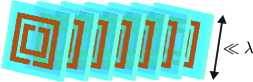
Figure 1: (Color online) Schematic of a one-dimensional magnetoinductive waveguide. The brown (dark gray) and blue (light gray) parts represent metal and dielectric, respectively.

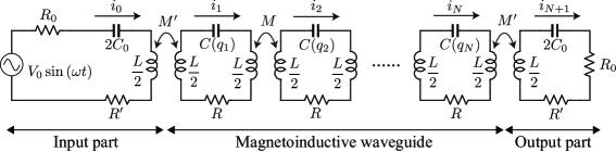
Figure 2: Electrical circuit model of a nonlinear magnetoinductive waveguide with input and output components. Mutual inductances except those between nearest neighbor loops are not shown to avoid complexity of the figure.

II Numerical analysis

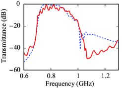
Figure 3: (Color online) Linear transmission spectra of the magnetoinductive waveguide obtained in the numerical analysis (dashed curve) and experiment (solid curve). The transmission spectrum in the numerical analysis is normalized to its maximum value.

We numerically investigate modulation instability in a one-dimensional magnetoinductive waveguide with third-order nonlinearity. To simplify the calculation, we analyze an electrical circuit model of the nonlinear magnetoinductive waveguide, as shown in Fig. 2. The circuit model is composed of a ladder of inductor-capacitor series resonant circuits that are coupled with each other via mutual inductances. The capacitors are assumed to exhibit third-order nonlinearity. Each end of the loop array represents a transmission line (with a characteristic impedance of $R_{0}$) and a transducer (with an inductance of $L/2$, a capacitance of $2C_{0}$, and a resistance of $R^{\prime}$) that couples the magnetoinductive waveguide to the transmission line. The resonant transducers are designed to suppress reflection at the interfaces between the waveguide and the transmission lines.Syms et al. (2010) The sinusoidal voltage source in the leftmost loop corresponds to an incident monochromatic wave. Applying Kirchhoff’s voltage law for the $n$th loop yields the following equation:

$$L\frac{{\mathrm{d}}i_{n}}{dt}+Ri_{n}+v_{n}+\sum_{u=1}^{U}M_{u}\left(\frac{{\mathrm{d}}i_{n+u}}{{\mathrm{d}}t}+\frac{{\mathrm{d}}i_{n-u}}{{\mathrm{d}}t}\right)=0,$$ (1)

where $M_{u}$ is the mutual inductance between the $n$-th loop and the $(n\pm u)$-th loop and $U$ is the upper limit of $u$ in the calculation. The voltages across the capacitors are assumed to be written as

$$v_{n}=\frac{q_{n}}{C(q_{n})}=\frac{q_{n}}{C_{0}}+\alpha q_{n}^{3},$$ (2)

where $C_{0}$ is the linear capacitance, $\alpha$ is a constant that represents the third-order nonlinearity, and ${\mathrm{d}}q_{n}/{\mathrm{d}}t=i_{n}$. The transmission characteristics of the electrical circuit model of the nonlinear magnetoinductive waveguide can be found by solving a set of simultaneous differential equation (1). We numerically solve Eq. (1) using the fourth-order Runge-Kutta method.

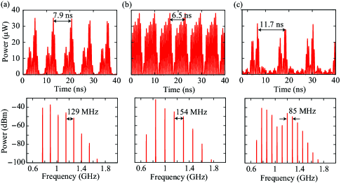
Figure 4: (Color online) Numerically calculated waveforms (upper row) and spectra (lower row) of the transmitted waves through the electrical circuit model of the nonlinear magnetoinductive waveguide for (a) $f=1.15\,{\mu\Omega\mathrm{GHz}}$, $P=17.4\,{\mu\Omega\mathrm{dBm}}$, (b) $f=1.15\,{\mu\Omega\mathrm{GHz}}$, $P=18.5\,{\mu\Omega\mathrm{dBm}}$, and (c) $f=1.20\,{\mu\Omega\mathrm{GHz}}$, $P=18.5\,{\mu\Omega\mathrm{dBm}}$.

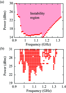
Figure 5: (Color online) Region where the modulation instability caused by the instantaneous third-order nonlinearity is observed. (a) Frequency dependence of threshold value of the source power in the numerical analysis. The instability region is shaded in light red (light gray). (b) Condition of the incident frequency and power in the experiment.

From a preliminary evaluation of the characteristics of the nonlinear split-ring resonator used in the experiment (next section), we determined the circuit constants as follows. The linear capacitance and nonlinear constant were, respectively, set to be $C_{0}=1.08\,{\mu\Omega\mathrm{pF}}$ and $\alpha=8.64\,{\mu\Omega\mathrm{mV/(pC)^{3}}}$ from the datasheet of the varactor diode (Infineon BBY52-02W) used as the nonlinear capacitor. The inductance ($L=27.5\,{\mu\Omega\mathrm{nH}}$) and resistance ($R=7.66\,{\mu\Omega\mathrm{O}}$) were determined from the linear capacitance, measured linear resonant frequency ($920\,{\mu\Omega\mathrm{MHz}}$), and linear resonance linewidth. The mutual inductances between the two loops were calculated from Neumann’s formulaStratton (1941) fitted to the experimental values, which were estimated from the frequency separation of the two resonance peaks of the two coupled split-ring resonators.Syms et al. (2006) For simplicity of calculation, the mutual inductances between the transducer and the other loops were set so that the coupling coefficient $\kappa^{\prime}_{u}=M^{\prime}_{u}/\sqrt{[L(L/2)]}$ was equal to $\kappa_{u}=M_{u}/L$. The upper limit of $u$ was set to be $U=10$, because $\kappa_{10}<\kappa_{1}/100$ and the $U$ dependence of the linear transmission spectrum of the electrical circuit model of the magnetoinductive waveguide was confirmed to be small in the case of $U>10$. The other parameters were set to be $R^{\prime}=R$, $N=25$, and $R_{0}=50.0\,{\mu\Omega\mathrm{O}}$. The dashed curve in Fig. 3 shows a linear transmission spectrum derived from the electrical circuit model as the power consumption of resistance $R_{0}$ in the rightmost loop. The transmission band in the linear region is found to be from 0.73 GHz to 0.88 GHz.

Figure 4 shows three examples of waveforms and spectra of the transmitted waves through the electrical circuit model of the nonlinear magnetoinductive waveguide for different incident frequencies $f$ and powers $P$. The transmitted waves are periodically modulated due to the modulation instability. While the waveform and spectrum of the transmitted wave are strongly dependent on the source frequency and power, the separation of the spectral peaks is of the order of 100 MHz in every case. Note that the generation of nonlinear waves is not derived from parametric four-wave mixing inside each separated split-ring resonator. Only the frequency components that satisfy the phase-matching condition in the magnetoinductive waveguide can be observed in the transmitted waves. That is, the frequencies of the spectral peaks of the transmitted waves are determined by the dispersion relation of the magnetoinductive waveguide.

Figure 5(a) shows the threshold value of the source power for generating the modulation instability as a function of the source frequency. The threshold becomes small in the range of about $1.0$–$1.2\,{\mu\Omega\mathrm{GHz}}$, which is slightly higher than the linear transmission band. This observation is intuitive because, as the incident power increases, the resonant frequency of the split-ring resonator shifts to higher frequency due to the third-order nonlinearityPoutrina et al. (2010) and the transmission band shifts to higher frequency.

III Experiment

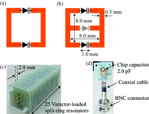
Figure 6: (Color online) (a) Varactor-loaded split-ring resonator with third-order nonlinearity and (b) that with a faster nonlinear response. The split-ring resonator is fabricated using an FR-4 printed circuit board, the thicknesses of the copper layer and the substrate of which are $35\,{\mu\Omega\mathrm{um}}$ and $1.6\,{\mu\Omega\mathrm{mm}}$, respectively. The black varactor diodes are Infineon BBY-52-02W and the gray diode is Rohm 1SS400. Photographs of (c) the magnetoinductive waveguide and (d) the resonant transducer connected to a coaxial cable.

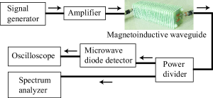
Figure 7: (Color online) Experimental setup for observing modulation instability in a magnetoinductive waveguide.

In this section we describe the experimental observation of modulation instability in the nonlinear magnetoinductive waveguide in the microwave region. Figure 6(a) shows a split-ring resonator loaded with two back-to-back varactor diodes. The split-ring resonator exhibits the third-order nonlinearity.Poutrina et al. (2010) Infineon BBY52-02W varactor diodes were used to realize high nonlinearity with low loss in the split-ring resonator. (The quality factor of the split-ring resonator is determined by the resistance of the varactor diodes rather than the radiation loss of the split-ring resonator.) Since the reverse current of the varactor diode is extremely small, the nonlinear response of the split-ring resonator is slow due to the accumulation of minority carriers. To solve this problem, we modified the structure of the split-ring resonator as shown in Fig. 6(b) and introduced another diode (Rohm 1SS400), whose reverse current is larger than that of the former diodes. The latter diode has little influence on the linear characteristics of the split-ring resonator. By arranging the 25 split-ring resonators axially with a separation of 2.9 mm as shown in Fig. 6(c), we constructed a nonlinear magnetoinductive waveguide with the third-order nonlinearity. To couple the magnetoinductive waveguide to coaxial cables, we used the resonant transducersSyms et al. (2010) shown in Fig. 6(d), whose inductance and capacitance were about half and twice that of the varactor-loaded split-ring resonator, respectively. The solid curve in Fig. 3 shows the linear transmission spectrum of the magnetoinductive waveguide measured using a network analyzer. The frequency range of the transmission band agrees well with that of the numerical calculation.

The experimental setup for observing modulation instability in the magnetoinductive waveguide is shown in Fig. 7. A continuous wave was generated from a microwave signal generator. The wave was amplified and then fed into the magnetoinductive waveguide. The transmitted wave was split into two halves by a power divider. One half was detected by a microwave diode detector to observe the envelope of the transmitted wave using an oscilloscope. The other half was fed into a spectrum analyzer.

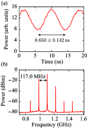
Figure 8: (Color online) Characteristics of the transmitted wave for $f=1100\,{\mu\Omega\mathrm{MHz}}$ and $P=26.5\,{\mu\Omega\mathrm{dBm}}$: (a) waveform of the envelope and (b) spectrum. The inverse of the modulation period, $(8.650\,{\mu\Omega\mathrm{ns}})^{-1}=115.6\,{\mu\Omega\mathrm{MHz}}$, is consistent with the separation of the spectral peaks.

We show three examples of transmitted waves through the nonlinear magnetoinductive waveguide for different incident frequencies $f$ and powers $P$. Figure 8 gives the measured characteristics of the transmitted wave for $f=1100\,{\mu\Omega\mathrm{MHz}}$ and $P=26.5\,{\mu\Omega\mathrm{dBm}}$. In the time domain, the transmitted wave is periodically modulated, and thus, the modulation instability occurs also in the experiment. In the spectral domain, spectral peaks appear at spacings of about 100 MHz, which is the same order as in the numerical calculation. Figure 9 shows the characteristics of the transmitted wave for $f=900\,{\mu\Omega\mathrm{MHz}}$ and $P=26.0\,{\mu\Omega\mathrm{dBm}}$. The modulation period is of the order of $100\,{\mu\Omega\mathrm{us}}$ and the frequency separation between the spectral peaks is of the order of $10\,{\mu\Omega\mathrm{kHz}}$. These values are of a different order of magnitude than those obtained from the numerical analysis. Figure 10 shows the characteristics of the transmitted wave for $f=980\,{\mu\Omega\mathrm{MHz}}$ and $P=26.0\,{\mu\Omega\mathrm{dBm}}$. Two kinds of spectral peaks spaced by about $100\,{\mu\Omega\mathrm{MHz}}$ and $10\,{\mu\Omega\mathrm{kHz}}$ are simultaneously observed.

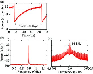
Figure 9: (Color online) Characteristics of the transmitted wave for $f=900\,{\mu\Omega\mathrm{MHz}}$ and $P=26.0\,{\mu\Omega\mathrm{dBm}}$: (a) waveform of the envelope, (b) spectrum, and (c) magnified spectrum around the peak. The inverse of the modulation period, $(72.48\,{\mu\Omega\mathrm{us}})^{-1}=13.8\,{\mu\Omega\mathrm{kHz}}$, is consistent with the separation of the spectral peaks. The difference between the peak values of the original and magnified figures is due to the limited resolution of the instruments.

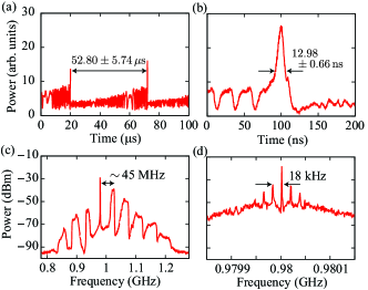
Figure 10: (Color online) Characteristics of the transmitted wave for $f=980\,{\mu\Omega\mathrm{MHz}}$ and $P=26.0\,{\mu\Omega\mathrm{dBm}}$: (a) waveform of the envelope, (b) magnified waveform around the peak, (c) spectrum, and (d) magnified spectrum around the largest peak. The inverse of the modulation period, $(52.80\,{\mu\Omega\mathrm{us}})^{-1}=18.9\,{\mu\Omega\mathrm{kHz}}$, is consistent with the narrower separation of the spectral peaks. The difference between the peak values of the original and magnified figures is due to the limited resolution of the instruments.

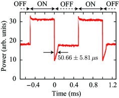
Figure 11: (Color online) Measured nonlinear relaxation characteristic of the varactor-loaded split-ring resonator. The incident frequency, power of the continuous wave, and power of the pulse-modulated wave during the pulse-on period are 1100 MHz, $17.0\,{\mu\Omega\mathrm{dBm}}$, and 31.0 dBm, respectively.

IV Comparison between numerical analysis and experiment

We have shown through the numerical calculation and experiment that modulation instability occurs in the nonlinear magnetoinductive waveguide. However, there are some discrepancies between the results of the numerical calculation and experiment. In the numerical calculation, there exist only spectral peaks spaced by about 100 MHz. In contrast, in the experiment, there exist spectral peaks spaced by about 10 kHz as well as 100 MHz. We explore the cause of the difference below.

The third-order nonlinear response is assumed to occur instantaneously in the numerical analysis. On the other hand, the varactor-loaded split-ring resonators used in the experiment show not only the instantaneous nonlinear response but also a delayed nonlinear response due to the small reverse current of the diodes. (Although we made the nonlinear response faster by introducing the auxiliary diode, the delayed nonlinear response still remains.) When a third-order nonlinear response of a material occurs noninstantaneously as well as instantaneously, the material will exhibit a Raman gain. If we assume that the delayed nonlinear response is described by an exponential relaxation function, the Raman gain takes a maximum value at frequencies spaced by the inverse of the relaxation time from the incident frequency.Stolen et al. (1989) Therefore, we can assume that the varactor-loaded split-ring resonator exhibits a delayed nonlinear response with a relaxation time that equals the modulation period.

To evaluate the nonlinear relaxation time of the fabricated split-ring resonator, we measured the envelope of the transmitted wave when a superposition of a pulse-modulated wave (high power) and a continuous wave (low power) was injected into a nonlinear magnetoinductive waveguide composed of one varactor-loaded split-ring resonator. An example of the measured envelope of the transmitted wave is shown in Fig. 11. During the turn-on transition, the amplitude of the envelope changes instantaneously. On the other hand, we observe a delayed nonlinear response with a relaxation time of about $50\,{\mu\Omega\mathrm{us}}$ during the turn-off transition. While the relaxation time strongly depends on the incident frequency and power, the order of the relaxation time agrees with that of the modulation period for some conditions. Therefore, we infer that it is the delayed nonlinear response that causes the narrowly separated ($\sim 10\,{\mu\Omega\mathrm{kHz}}$) spectral peaks—in other words, the long modulation period ($\sim 100\,{\mu\Omega\mathrm{us}}$) in the experiment. The asymmetry in the relaxation phenomenon is due to the asymmetry of the current flow in the diodes. If we make a strict electrical circuit model of the split-ring resonator used in the experiment, we could reproduce the experimentally observed phenomenon using the numerical calculation shown in the previous section. However, we do not perform this simulation here because the strict modeling is beyond the scope of the present work.

From the above discussion, it is found that there exist instantaneous and noninstantaneous third-order nonlinearities in the varactor-loaded split-ring resonators and each nonlinearity can cause a modulation instability in the nonlinear magnetoinductive waveguide. This implies that the modulation instability is caused by the instantaneous or noninstantaneous nonlinearity in the case of Fig. 8 and Fig. 9, respectively, and by both kinds of nonlinearities in the case of Fig. 10.

In Fig. 5(b) we show the condition of the incident frequency and power for generating the modulation instability caused by the instantaneous nonlinearity in the experiment to compare the experimental and numerical results. We examined the condition by increasing the incident power from 12.5 dBm to 31.0 dBm with 0.5 dBm steps in the frequency range 700–1400 MHz with steps of 10 MHz. Since the separation of the spectral peaks is of the order of 100 MHz and 10 kHz in the case of the modulation instability caused by the instantaneous and noninstantaneous nonlinearity, respectively, we consider that the modulation instability is caused by the instantaneous nonlinearity if the separation of the spectral peaks is larger than 10 MHz.

While the measured instability condition [Fig. 5(b)] roughly agrees with the numerical calculation [Fig. 5(a)], there are two minor discrepancies between them. First, in the experiment, the threshold of the incident power varies rapidly with respect to the incident frequency. Second, there exist some conditions where, although the incident power exceeds the threshold value, modulation instability does not occur. The former difference could be induced because the reflection at the transducer in the experiment is larger than that in the numerical calculation. The electromagnetic energy density in the waveguide increases or decreases depending on the incident frequency due to the Fabry-Perot effect and thus the threshold oscillates. The latter difference may be caused by the power dependence of the effective resistance of the varactor diode. With increasing incident power, the effective resistance increases and the transmittance in the transmission band decreases (not shown). There may be the cases where the increase of the propagation loss becomes larger or smaller than the increase of the gain of the modulation instability when the incident power increases. The Raman gain in the experiment may also be one of the causes of the differences.

V Conclusion

We have shown through a numerical analysis of an electrical circuit model and an experiment in the microwave region that modulation instability occurs in a magnetoinductive waveguide with third-order nonlinearity. While the condition for generating the modulation instability in the experiment roughly agrees with that in the numerical calculation, there are some discrepancies in the characteristics of the modulation instability. The experimental result implies that the difference is due to the noninstantaneous nonlinearity, which was not considered in the numerical analysis. This inference could be confirmed by making a strict electrical circuit model of the varactor-loaded split-ring resonator or by a full wave simulation using a finite-difference time-domain methodTaflove and Hagness (2005) taking both the instantaneous and noninstantaneous nonlinearities into account. Our study in the microwave region can be extended to the terahertz and optical regions using micro- and nanofabrication technologies.