First results from a study of DIBs with thousands of high-quality massive-star spectra

Abstract

We are using five different surveys to compile the largest sample of diffuse interstellar band (DIB) measurements ever collected. GOSSS is obtaining intermediate-resolution blue-violet spectroscopy of $\sim$2500 OB stars, of which 60% have already been observed and processed. The other four surveys have already collected multi-epoch high-resolution optical spectroscopy of 700 OB stars with different telescopes, including the 9 m Hobby-Eberly Telescope in McDonald Observatory. Some of our stars are highly-extinguished targets for which no good-quality optical spectra have ever been published. For all of the targets in our sample we have obtained accurate spectral types, measured non-DIB ISM lines, and compiled information from the literature to calculate the extinction. Here we present the first results of the project, the properties of twenty DIBs in the 4100-5500 Å range. We clearly detect a couple of previously elusive DIBs at 4170 Å and 4591 Å; the latter could have coronene and ovalene cations as carriers.

1 The project

The Galactic O-Star Spectroscopic Survey (GOSSS, Maíz Apellániz et al. 2011, Sota et al. 2011) is obtaining long-slit, $R\sim$2500, blue-green spectroscopy of $\sim$2500 massive stars in both hemispheres, including all known O stars with $B<12$. Its main purpose is to characterize the O-star population in the solar neighborhood by providing accurate spectral types for all of the observed targets. We currently have spectra for 1592 stars and we plan to reach 2500 within two years.

Four other surveys are obtaining high-resolution spectroscopy of a subsample of the GOSSS stars with the purposes of doing detailed atmospheric modeling and calculating the orbits of the spectroscopic binaries. Three of those surveys, OWN (Barbá et al. 2010), IACOB (Simón-Díaz et al. 2011a, 2011b), and NoMaDS (Maíz Apellániz et al. 2012), have been described elsewhere. The fourth one, CAFÉ-BEANS (Calar Alto Fiber-fed Échelle Binary Evolution Andalusian Survey, P.I.: Ignacio Negueruela), is obtaining multi-epoch $R=$ 65 000 spectroscopy of northern stars using the CAFÉ spectrograph at the 2.2 m telescope at Calar Alto (Aceituno et al. 2012).

The original goal of these surveys was to study the stars but they also contain an unprecedented amount of information on optical ISM lines. That led us to start a parallel project to obtain and process such information. In this first analysis we study the properties of the DIBs seen in the GOSSS data.

Table 1. GOSSS extincted and reference stars used in this work.

ID	Extincted star	Spectral type	$E(B-J)$
1	Cyg OB2-12	B5 Ia	10	.38
2	ALS 19 626	B0 Ia	8	.61
3	2MASS	B0 Ia	8	.33
	J20333821+4041064
4	ALS 21 079	O7 Ib-II(f)	7	.64
5	Cyg OB2-22 B	O6 V((f))	7	.56
6	Cyg OB2-22 A	O3 If*	7	.51
7	ALS 15 114	O7.5 Vz	7	.50
8	2MASS	O6.5 III(f)	7	.12
	J20344410+4051584
9	ALS 18 747	O5.5 Ifc	5	.94
ID	Reference star	Spectral type	$E(B-J)$
1	$\eta$ CMa	B5 Ia	0	.37
2	HD 91 969	B0 Ia	0	.82
3	HD 91 969	B0 Ia	0	.82
4	HD 94 963	O7 II	0	.68
5	HDE 303 311	O6 V	1	.53
6	$\zeta$ Pup	O4 I(n)f	0	.07
7	HD 53 975	O7.5 Vz	0	.62
8	HD 152 723 AaAb	O6.5 III(f)	1	.45
9	HD 93 632	O5.5 Ifc	2	.33

  Table 2. Properties of the DIBs measured in this work using Gaussian fits. The first column gives the group ID (some DIBs were fitted together), the next two give the fit results, the fourth one the average equivalent widths of the used stars, and the last one the number of stars used. gr. $\lambda_{\rm c}$ (Å) FWHM (Å) EW (Å) $n_{\rm st}$ 1 4179.48$\pm$0.61 21.88 $\pm$1.73 0.62$\pm$0.14 8 2 4427.94$\pm$0.11 24.15 $\pm$0.30 3.55$\pm$0.68 9 3 4501.67$\pm$0.09 3.24 $\pm$0.40 0.17$\pm$0.04 9 4 4591.19$\pm$0.56 24.95 $\pm$1.58 0.68$\pm$0.25 6 5 4726.70$\pm$0.05 3.88 $\pm$0.30 0.28$\pm$0.05 9 6 4761.12$\pm$0.27 19.72 $\pm$1.06 0.58$\pm$0.09 9 6 4762.36$\pm$0.09 2.69 $\pm$0.48 0.10$\pm$0.01 9 6 4779.69$\pm$0.21 5.48 $\pm$0.57 0.13$\pm$0.02 9 7 4879.83$\pm$0.16 11.51 $\pm$0.63 0.43$\pm$0.07 7 7 4887.43$\pm$0.65 39.75 $\pm$1.14 2.16$\pm$0.36 7 8 4963.85$\pm$0.15 2.62 $\pm$0.66 0.06$\pm$0.02 8 9 4984.59$\pm$0.23 1.33 $\pm$1.29 0.02$\pm$0.01 8 10 5109.66$\pm$0.43 14.91 $\pm$1.34 0.23$\pm$0.08 6 11 5155.99$\pm$0.49 15.97 $\pm$1.50 0.14$\pm$0.03 7 12 5236.29$\pm$0.24 2.27 $\pm$0.77 0.06$\pm$0.02 5 12 5245.43$\pm$0.57 7.26 $\pm$1.56 0.08$\pm$0.03 5 13 5363.52$\pm$0.13 2.74 $\pm$0.55 0.07$\pm$0.01 7 14 5449.83$\pm$0.22 14.06 $\pm$0.61 0.48$\pm$0.13 8 15 5487.23$\pm$0.12 6.63 $\pm$0.33 0.35$\pm$0.05 6 15 5494.29$\pm$0.26 1.90 $\pm$0.96 0.04$\pm$0.01 6

2 4100-5500 Å DIB properties

We selected 9 stars observed by GOSSS with high extinction, good S/N spectra, and coverage of the full 3900-5500 Å range (Table 1). For each star we selected a corresponding GOSSS star with low extinction and similar spectra type in order to apply the traditional pair method, in which the low-extinction spectrum is subtracted from the high-extinction one in order to eliminate the stellar contribution. The spectra were put in the ISM reference system using the Ca ii $\lambda$3934 line. The average profile was then calculated for each DIB by selecting the stars in the sample with the largest EWs, normalizing by it, and calculating the mean and standard deviation of the spectra at each wavelength. The result was fit using either Gaussian and Lorentzian profiles (multiple in the case where DIBs overlap so they must be fitted in groups). Finally, the instrumental width was subtracted to the fit FWHM. Results for the Gaussian fits are shown in Table 2.

• We clearly detect the seldom seen 4179 Å broad DIB (Knoechel & Moffat 1982, Jenniskens & Désert 1994; Fig. 1).

• The broad intense 4428 Å DIB is better fit by a Lorentzian than a Gaussian (see Snow et al.. 2002). However, the differences are small and the broad Lorentzian wings make rectification difficult in practice, so Gaussian fits are less noisy for most data.

• We detect the previously elusive 4591 Å broad DIB, which could be produced by coronene (C₂₄H₁₂) and ovalene (C₃₂H₁₄) cations (Ehrenfreund et al. 1995, Fig. 1).

• The 4770 Å region requires a fit with two narrow and one broad DIBs (Fig. 1).

• The 4880 Å region requires a fit with one broad and one intermediate DIBs (Fig. 1).

• The 5110 Å DIB shows a possible additional component in its left wing.

• There may be a broad component around the 5364 Å DIB (not measured).

• At this resolution the two narrow DIBs to the left and right of He ii $\lambda$5412 are blended with the stellar line and are not analyzed here.

• The 5240 Å region shows two clearly separated components at this resolution.

• The 5490 Å region shows two clearly separated components at this resolution.

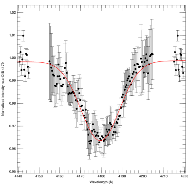
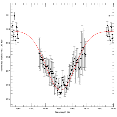
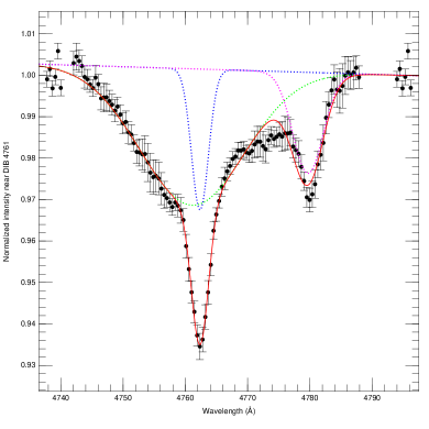
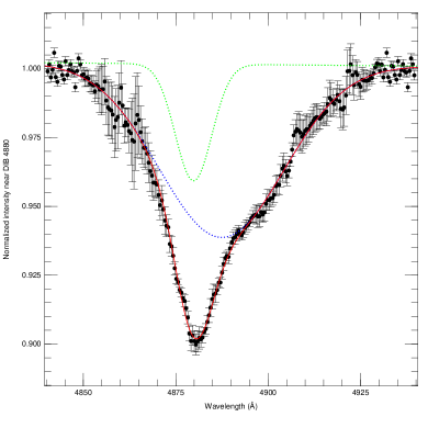
Figure 1: Gaussian fits for DIB groups 1, 4, 6, and 7. Error bars show the standard deviation of the average profile normalized by EW. Dotted lines are used for individual components.

References

- [Aceituno et al. (2012)] Aceituno, J., et al. 2012, A&A 552, A31
- [Barbá et al. (2010)] Barbá, R. H. et al. 2010, Revista mexicana de astronomía y astrofísica (serie de conf.) 38, 30
- [Ehrenfreund et al. (1995)] Ehrenfreund, P. et al. 1995, A&A 299, 213
- [Jenniskens & Désert (1994)] Jenniskens, P. & Désert, F.-X. 1994, A&AS 106, 39
- [Knoechel & Moffat (1982)] Knoechel, G. & Moffat, A. F. J. 1982, A&A 110, 263
- [Maíz Apellániz et al. (2011)] Maíz Apellániz, J. et al. 2011, Highlights of Spanish Astrophysics VI, 467
- [Maíz Apellániz et al. (2012)] Maíz Apellániz, J. et al. 2012, ASP Conference Series 465, 484
- [Simón-Díaz et al. (2011a)] Simón-Díaz, S., Castro, N., García, M., & Herrero, A. 2011a, IAU Symposium 272, 310
- [Simón-Díaz et al. (2011b)] Simón-Díaz, S. et al. 2011b, arXiv 1109.2665
- [Snow et al. (2002)] Snow, T. P., Zukowski, D. & Massey, P. 2002, ApJ 578, 877
- [Sota et al. (2011)] Sota, A. et al. 2011, ApJS 193, 24