Electron-phonon interaction on the surface of a 3D topological insulator

Abstract

We analyze the role of a Rayleigh surface phonon mode in the electron-phonon interaction at the surface of a 3D topological insulator. A strong renormalization of the phonon dispersion, leading eventually to the disappearance of Rayleigh phonons, is ruled out in the ideal case of a continuum long-wavelength limit, which is only justified if the surface is clean and defect free. The absence of backscattering for Dirac electrons at the Fermi surface is partly responsible for the reduced influence of the electron-phonon interaction. A pole in the dielectric response function due to the Rayleigh phonon dispersion could drive the electron-electron interaction attractive at low frequencies. However, the average pairing interaction within the weak coupling approach is found to be too small to induce a surface superconducting instability.

I Introduction

Topological insulators (TI) have attracted a great deal of attention in recent times Zhang et al. (2009); Hasan and Kane (2010). Their most significant feature is the existence of topologically protected surface states. In this context, the electron-phonon (e-ph) interaction at the surface of a 3D topological insulator is particularly relevant, as it could make a significant contribution to the transport properties of the surface states Giraud and Egger (2011); Zhu et al. (2011, 2012); Pan et al. (2012). Experimental evidence is ambiguous. ARPES measurements reveal small effects on surface electrons Pan et al. (2012), suggesting that there is a negligible interaction between electrons and surface phonons at the boundary of a 3D TI. On the other hand, a strong coupling of phonons with surface electrons is extracted from measurements of surface phonon spectra in Bi₂Se₃, leading to a strong Kohn anomaly for transvserse optical surface phonons, while there is no evidence of a Rayleigh acoustical branch Zhu et al. (2011) which would usually be expected to exist in systems with a free surface Zhu et al. (2012). A possible explanation given for the latter feature is a different coupling between planes in the quintuple layer of Bi₂Se₃.
Here we explore a different scenario and assume that the Rayleigh acoustical branch is well defined up to large enough $\vec{q}$ wave vectors parallel to the surface and we would like to check its renormalization due to the electronic states at the surface. This assumption motivates a study of the electron-phonon interaction at the surface of a 3D TI. Our low-energy theory involves a single Dirac cone at the $\Gamma$ point for surface electrons. Up to the linear order in the strain vector u the main contribution to the e-ph interaction is the deformation potential seen by the surface electrons (see Appendix A). In this respect, the crucial quantity that determines the strength of the e-ph coupling is the $q=|\vec{q}|$ vector dependent structure factor $\Lambda_{l}\left(q\right)$, quantifying the localization of the phonon mode at the surface and its overlap with the surface electron density. The typical decay length of the Rayleigh mode away from the surface $\propto 1/q$ has to be compared with the length scale appearing in the screened electronic polarization operator ${\cal{P}}$. While the bare electronic polarization operator may be large even at small $q$ values, the screening in the RPA approximation turns out to be very effective up to $q\sim\alpha_{FS}k_{F}/2\pi$, which is a transferred momentum spanning a large portion of the Fermi surface. Here $k_{F}$ is the Fermi wave vector, $\alpha_{FS}$ is the effective fine structure constant $\alpha_{FS}=e^{2}/\epsilon\hbar v_{F}\sim 0.1$ and $\epsilon\sim 50$ is the average bulk dielectric constant V. Sandomirsky and Schlesinger (2001); Greenaway and Harbeke (1965). At larger momenta, $\Lambda_{l}\left(q\right)$ is heavily suppressed, if it mimicks an ideal continuum medium in the long wavelength limit (see Eq.(5)), leading to a reduction of e-ph interaction. It follows that in this case a small renormalization of the phonon frequency and of the electronic plasma surface mode is produced. However, the ideal limit discussed up to this point for $\Lambda_{l}\left(q\right)$ may be questionable, in view of the scattering by impurities and defects at the surface, and we also show that a different $q$ dependence of $\Lambda_{l}\left(q\right)$ may be quite critical for the survival of the Rayleigh mode. We investigate the limiting case $\Lambda_{l}(q)\sim 1$, analyzing a possible reconstruction of the surface.

In Section II we introduce the model and evaluate the matrix element of the e-ph interaction. In Section III we discuss the damping of the Rayleigh mode, the quality factor and the remote possibility of a softening of the phonon Rayleigh mode in the continuum model. In Section IV the influence of the e-ph interaction in the electron-electron (e-e) scattering is analyzed within the RPA approximation. A short summary of the conclusions is reported in Section V.

Appendix A elaborates on the symmetry properties of the e-ph coupling Hamiltonian and proves that the occurence of the Dirac cone at the $\Gamma$ point constrains the e-ph interaction to a featureless deformation potential.

Appendix B develops a perturbative approach in the continuum elastic dynamics of the surface displacements to deal with a strong anisotropy of the elastic constants while approaching the outermost layers of the surface. The derivation shows that although the sound velocity is softened, the mode always remains well defined.

II The model

The low energy effective Hamiltonian describing the electrons interacting with the phonons is $\mathcal{H}=\mathcal{H}_{0}+\mathcal{H}_{el-ph}$, where $\mathcal{H}_{0}=-i\hbar v_{F}\boldsymbol{\sigma}\cdot\nabla$ is the free Dirac Hamiltonian in 2+1 dimensions for the surface electronic states and $\mathcal{H}_{el-ph}$ is the e-ph interaction. In second quantization

$$\begin{split}\mathcal{H}_{0}-\mu\mathcal{N}&=\sum_{k,s=\pm}\epsilon_{ks}c^{\dagger}_{k,s}c_{k,s},\quad\epsilon_{ks}=sv_{F}|k|-\mu\\ \mathcal{H}_{el-ph}&=\sum_{\boldsymbol{k},\boldsymbol{q},\omega,s}M_{ss}(q)(a_{q}+a^{\dagger}_{q})c^{\dagger}_{\textbf{k+q},s}c_{\textbf{k},s}+h.c..\end{split}$$ (1)

Here $s=\pm$ labels the helicity of surface states $\left|\textbf{k},s\right>$, $\mu=\hbar v_{F}k_{F}$ is the chemical potential and $v_{F}$ is the Fermi velocity ($v_{F}=4.36\times 10^{5}m/s$ for Bi₂Te₃). In systems with a free surface, the Rayleigh mode localized at the surface can be expected to be strongly coupled to the surface states. In the following, we will focus on its contribution to the e-ph interaction. Using linear elasticity theory for an isotropic continuum with stress-free boundary conditions at $z=0$, the Rayleigh mode has a linear dispersion relation $\omega_{q}^{(0)}=c_{R}q$ with velocity $c_{R}=0.89\>c_{t}$ Ezawa (1971); Landau and Lifshitz (1975), where the $c_{l,t}$ are the longitudinal and transverse phonon velocities as determined by elasticity theory. Here $c_{R}/v_{F}\approx 3\times 10^{-3}$. The matrix element of the e-ph interaction, $M_{ss^{\prime}\vec{k}}(\vec{q})$, can be written in terms of the displacement field operator U, as a linear combination of the components of the strain tensor:

$$M_{ss^{\prime}\vec{k}}(\vec{q})=\alpha\left<\textbf{k}+\textbf{q},s|A_{ij}\partial_{i}U_{j}|\textbf{k},s^{\prime}\right>$$ (2)

The generic matrices $A_{ij}$ are determined so that the interaction is compatible with the symmetries of the system. As shown in Appendix B, the high symmetry of the $\Gamma$ point implies that the only possible coupling is with the trace of the strain tensor through the identity matrix $A_{ij}=\delta_{ij}$. Since the e-ph interaction conserves helicity and is independent of it, we drop the label $s$ henceforth. At k close to the $\Gamma$ point, the matrix element of the e-ph interaction reads

$$M(q)=\alpha\>\sqrt{\frac{C}{q\mathcal{A}}}\left(\frac{\omega_{q}^{(0)}}{c_{l}}\right)^{2}\sqrt{\frac{\hbar}{2\rho_{M}\omega_{q}^{(0)}}}\>\Lambda_{l}(q).$$ (3)

Here $\mathcal{A}$ is the unit cell area, while the constant $\alpha$ characterizes the strength of the e-ph coupling Giraud and Egger (2011). In the case of Bi₂Te₃ the estimated value for $\alpha$ is 35eV, as extracted from first principle calculations including static screening effectsHuang and Kaviany (2008). The mass density of Bi₂Te₃ isGiraud and Egger (2011) $\rho_{M}=7860\text{Kg/ m}^{3}\>$ . The coefficient $C$ is completely determined by the velocities for longitudinal and transverse phonons $c_{l}=2800m/s$ and $c_{t}=1600m/s$, through the dimensionless quantities $\lambda_{l}=\sqrt{1-c_{R}/c_{l}}$ and $\lambda_{t}=\sqrt{1-c_{R}/c_{t}}$,

$$\frac{1}{C}=\lambda_{l}-\lambda_{t}+\frac{(\lambda_{l}-\lambda_{t})^{2}}{2\lambda_{l}^{2}\lambda_{t}}$$ (4)

and its value for Bi₂Te₃ is 1.2. As the length scale for the penetration of the surface states inside the bulk is $\hbar v_{F}/\Delta$, where $\Delta$ is the gap in the bulk spectrum, the spatial overlap in the $z$-direction of the electronic surface density with the wavefunction of the Rayleigh phonons in the ideal case is given by:

$$\Lambda_{l}(q)=\frac{2\Delta}{\hbar v_{F}}\int_{0}^{\infty}\!\!\!\!\!\!\!e^{-2\Delta z/\hbar v_{F}-\lambda_{l}qz}dz=\frac{\Delta}{\Delta+\lambda_{l}\hbar v_{F}|q|/2}\>.$$ (5)

This expression does not account for surface defects such as edge dislocations or localized scattering centers, which are likely to be present e.g. due to Te vacancies. It can be expected that the most relevant transferred momenta $q$ for the e-ph interaction are the ones connecting points at the Fermi surface up to $q\sim 2k_{F}$. Due to the absence of backscattering at the ideal surface of the TI, it turns out that scattering with small $q$ has a major role. The actual $q$ dependence of $\Lambda_{l}(q)$ is quite critical for the strength of the e-ph coupling, as will be shown in the following. In particular $\Lambda_{l}(q)$ attains the largest value ($\Lambda_{l}(q)\approx 1$) when $q\ll\Delta/\hbar v_{F}$.

III Effects of electrons on phonons

Electronic screening effects can be taken into account, within the RPA approximation. The electronic polarization operator takes the formMahan (1990)

$$\mathcal{P}(q,\omega)=\frac{P(q,\omega)}{1-v_{q}P(q,\omega)}\>,$$ (6)

where $P(q,\omega)$ is the bare polarization operator per unit area and $v_{q}=e^{2}/2\epsilon q$ is the 2-D electron-electron (e-e) interaction. To investigate the effects of electrons on phonons at the surface of a TI, we first study the phonon damping, defined through the imaginary part of (6) as $\Gamma_{q}=|M(q)|^{2}\text{Im}\mathcal{P}(q,\omega)$ [see Sec. III.1]. The real part of (6), on the other hand, determines the correction to the phonon dispersion $\Delta E=|M(q,\omega)|^{2}\text{Re}\mathcal{P}(q,\omega)$ [see Sec. III.2].

III.1 Phonon damping and quality factor

The phonon damping is calculated as $\Gamma_{q}=|M(q)|^{2}\text{Im}\mathcal{P}(q,\omega)$, where $M(q)$ is the e-ph matrix element given in Eq.(3). In the small $q$ limit, with the frequency $\omega$ satisfying the inequalities

$$\frac{\hbar\omega}{\hbar v_{F}q}\ll 1\ll\frac{\mu}{\hbar v_{F}q}\>,$$ (7)

the bare electronic polarization operator per unit area, $P(q,\omega)$, has the imaginary part

$$\text{Im}P(q,\omega)=\frac{1}{4}\frac{\omega}{\hbar v_{F}^{2}}\sqrt{\left(\frac{2\mu}{\hbar v_{F}q}\right)^{2}-1}\>,$$ (8)

which can be quite large. Within the RPA approximation, we obtain for the full polarization operator

$$\text{Im}\mathcal{P}(q,\omega)=\begin{cases}\frac{\omega}{\hbar v_{F}^{2}\alpha_{FS}}\frac{q}{2k_{F}}\>\>\text{for}\;\;q<\frac{\alpha_{FS}k_{F}}{2\pi}\\ \\ \frac{1}{4}\frac{\omega}{\hbar v_{F}^{2}}\sqrt{\left(\frac{2\mu}{\hbar v_{F}q}\right)^{2}-1}\>\>\text{for}\;\;q>\frac{\alpha_{FS}k_{F}}{2\pi}.\end{cases}$$ (9)

In the limit $q<k_{F}$, the phonon decay rate $\Gamma_{q}$ is

$$\Gamma_{q}=\begin{cases}\frac{\pi}{8\alpha_{FS}}\>K\left(k_{F}\right)\>\frac{(\hbar\omega^{(0)}_{q}\Lambda_{l}(q))^{2}}{\mu}\>\frac{q^{2}}{k_{F}^{2}},\>\>\text{for}\;\;q<\frac{\alpha_{FS}k_{F}}{2\pi}\\ \\ \frac{\pi}{8}\>K\left(k_{F}\right)\>\frac{(\hbar\omega^{(0)}_{q}\Lambda_{l}(q))^{2}}{\mu}\>\>\text{for}\;\;q>\frac{\alpha_{FS}k_{F}}{2\pi}\>.\end{cases}$$ (10)

In our case, the effective fine structure constant, $\alpha_{FS}=e^{2}/\epsilon\hbar v_{F}$, is quite large, typically $\sim 0.1$ . This implies that the damping remains rather small (of order $q^{2}/k_{F}^{2}$) up to relatively high values of $q$. The dimensionless quantity

$$K(k_{F})=\frac{2\alpha^{2}C}{\pi}\frac{c_{R}^{2}}{v_{F}c_{l}}\frac{k_{F}^{2}}{\hbar\rho_{M}c_{l}^{3}}=2.35\;\text{nm}^{2}k_{F}^{2},$$ (11)

plays a central role in determining the features of the e-ph interaction at the surface of the TI. Its value is strongly dependent on the Fermi wave vector. As the linewidth vanishes for $q\rightarrow 0$, the Rayleigh phonons are well defined at small wave vectors. The quality factor $Q=\hbar\omega_{q}/\Gamma_{q}$, measuring the broadening of the phonon energy, is plotted in Fig. 1, also for larger wave vectors $q$. The nature of the divergence of $Q$ at $q=2k_{F}$ is quite specific to TIs, since $q=2k_{F}$ implies backscattering, which is suppressed by the orthogonality of the initial and final spin states.

III.2 Renormalization of the phonon dispersion

To investigate the renormalization of the phonon dispersion by the electronic screening, we calculate the real part of polarization operator $\mathcal{P}(q,\omega)$ in the static limit, $\omega\rightarrow 0$. Again, we find that its bare value $P(q,0)=-k_{F}/2\pi\hbar v_{F}$ is relatively large, while it is heavily suppressed by screening. The RPA approximation yelds

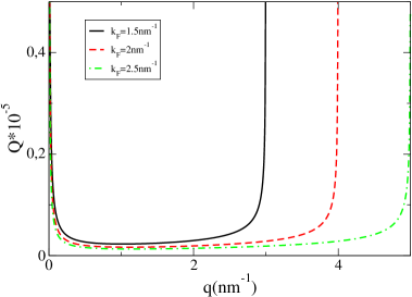
Figure 1: (Color Online) Quality factor $Q$ as a function of momentum $q$ for different values of the Fermi wave vector: $k_{F}=1\;\text{nm}^{-1}$ (black, full line), $k_{F}=1.5\;\text{nm}^{-1}$ (red, dashed line), and $k_{F}=2\;\text{nm}^{-1}$ (green, dashed-dotted line).

$$\mathcal{P}(q,0)=-\frac{k_{F}}{2\pi\hbar v_{F}}\>\mathcal{F}\left(q\right),$$ (12)

where $\mathcal{F}(q)$ is given by

$$\mathcal{F}(q)=\frac{\tilde{q}^{2}}{2}\frac{2-\tilde{q}\>\Theta(\tilde{q}-1)G_{<}\left(1/\tilde{q}\right)}{4\tilde{q}+\alpha_{FS}\left\{2-\tilde{q}\>\Theta(\tilde{q}-1)G_{<}\left(1/\tilde{q}\right)\right\}}\>.$$ (13)

Here $\tilde{q}=q/2k_{F}$ and $G_{<}(x)=x\sqrt{1-x^{2}}-\arccos x$. Its limiting form for $\tilde{q}\ll 1$ is $\mathcal{F}(q)=\frac{\tilde{q}^{2}}{2}\left[\alpha_{FS}+2\tilde{q}\right]^{-1}$.

The correction to the phonon dispersion, $\Delta\omega_{q}=|M(q)|^{2}\mathcal{P}(q,0)/\hbar$, gives the renormalization

$$\omega_{q}=\omega_{q}^{(0)}\left[1-\>\frac{K(k_{F})}{4}\>\Lambda_{l}^{2}(q)\>\mathcal{F}(q)\right],$$ (14)

which is plotted in Fig. 2 versus $q$ for $\alpha=35\;\text{eV}$ and two values of $k_{F}=1\;\text{nm}^{-1}$ (full line), $2.5\;\text{nm}^{-1}$ (dashed line). The inset shows that a renormalization of the phonon velocity only occurs for unrealistically large values of the e-ph coupling $\alpha=105\;\text{eV}$ (black full line), $210\;\text{eV}$ (red dashed line), $227.5\;\text{eV}$ (green dashed dotted line). However, the dispersion is quite sensitive to changes in the $q$ dependence of the structure factor. This can be seen from the dashed dotted curve in the main panel which is plotted for $\alpha=35\;\text{eV}$ and $k_{F}=1\;\text{nm}^{-1}$, by setting a flat structure factor $\Lambda_{l}(q)=1$.

In wide gap TIs, the spatial decay of the electronic surface states and of the Rayleigh modes can occur on comparable scales, leading to $\Lambda_{l}(q)\approx 1$. In this case, the softening of the mode could give rise to a lattice instability at some finite wave vector $q_{c}$. This critical value of $q$ depends on material parameters, such as the deformation potential and the sound velocity, and it is also a function of the doping: $q_{c}$ decreases with increasing $k_{F}$, eventually reaching a constant value $q_{c}^{*}$ fixed by the coupling constant $K(k_{F})$

$$q_{c}^{*}=4k_{F}\sqrt{\frac{\alpha_{FS}}{K(k_{F})}}.$$ (15)

However the formation of a scalar potential superlattice would weaken the screening and eventually compete with the occurrence of the instability itself. This is because a possible reconstruction would reduce heavily the electronic density of states at $q_{c}$, assumed to be close to $k_{F}$ (see Refs. Park et al., 2008; Guinea and Low, 2010; Yankowitz et al., 2012 for similar effects in graphene). A lattice instability in wide gap TIs, induced by the Rayleigh mode at momentum $q_{c}\neq k_{F}$ should be measurable in STM experiments Yankowitz et al. (2012) and would also modify the electronic transport properties.

A signature of the absence of the backscattering induced by the topological protection of the surface states shows up in a milder Kohn anomaly at $q=2k_{F}$, with respect to the one typical of a conventional two-dimensional electron gas. The nonanalyticity is not recognizable in the dispersion itself, but it appears as a kink in the first derivative, as shown in Fig. 2$(b)$ for three values of $k_{F}$ and $\alpha=35\;\text{eV}$. A sharp singularity only develops in the second derivative of the phonon dispersion, as shown in the inset of Fig. 2$(b)$.

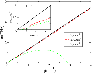
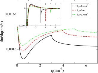
Figure 2: (Color online) $(a)$ Main Panel: Plot of the phonon dispersion $\omega_{q}$ given by eq.(14), for $\alpha=35eV$. The full line and the dashed line are for $k_{F}=1\text{nm}^{-1}$ and $k_{F}=2.5\text{nm}^{-1}$, respectively. The dashed-dotted curve is obtained for $k_{F}=1\text{nm}^{-1}$, by setting $\Lambda_{l}(q)=1$. Inset: The phonon frequency at $k_{F}=1.5\;\text{nm}^{-1}$ (in units $v_{F}k_{F}$) versus $q$, for different values of the strength of the deformation potential $\alpha=105\text{eV}$ (black full line), $210\text{eV}$(red broken line), $227.5\text{eV}$ (green dashed dotted line). $(b)$ Plot of the first derivative of $\omega_{q}$ versus $q$, for $\alpha=35eV$ and various $k_{F}$ values. The discontinuity at $q=2k_{F}$ signals the Kohn anomaly. The inset shows the corresponding marked discontinuities in the second derivative.

IV Effects of phonons on electrons

We now consider the renormalization of the bare e-e interaction $v_{q}$ by the e-ph interaction. The screened e-e potential takes the form $V(q,\omega)=\tilde{v}(q,\omega)/\epsilon(q,\omega)$, involving the propagator of the acoustic Rayleigh mode, $D^{(0)}(q,\omega)$,

$$\tilde{v}(q,\omega)=v_{q}+|M(q)|^{2}\>D^{(0)}(q,\omega)\>,$$ (16)

and the dielectric function

$$\frac{\epsilon(q,\omega)}{\epsilon}=1-\tilde{v}(q,\omega)\>P(q,\omega)\>.$$ (17)

The static limit $\epsilon(q,0)$ diverges for $q\rightarrow 0$ due to the metallic nature of the system. The zeroes of $\epsilon(q,\omega)$ determine the plasmon dispersion relation. The corrections to the bare plasmon dispersion

$$\omega^{(0)}_{p}(q)=\left(\alpha_{FS}\>\frac{v_{F}^{2}k_{F}}{4\pi}\>q\right)^{1/2}.$$ (18)

are quite small, as can be checked by using the approximate form of the polarization operator $P(q,\omega)\approx\mu q^{2}/4\pi\hbar^{2}\omega^{2}$, which is adequate in the limit

$$1\ll\frac{\hbar\omega}{\hbar v_{F}q}\ll\frac{\mu}{\hbar v_{F}q}.$$ (19)

The influence of the e-ph coupling on the e-e interaction can only be found at low $\omega$ values, when the transferred momentum matches the phonon dispersion. A color plot of the effective interaction at small $\omega$’s, in the plane $\omega/q$, is shown in Fig.3(a). We have plotted the dimensionless product $\rho\left(E_{F}\right)\>V(q,\omega)$, where $\rho(E_{F})=k_{F}/2\pi\hbar v_{F}$ is the density of states at the Fermi level, per spin direction. A cross section of the plot, marked by the black line in Fig. 3(a) (at $\omega/v_{F}k_{F}=0.005$), is reported in Fig. 3(b). The plot shows the sharp change of sign of the interaction in crossing the phonon dispersion.

It is interesting to inquire whether an instability to surface superconductivity in a TI as Bi₂Se₃ or Bi₂Te₃ could be triggered by the e-ph interaction mediated by the Rayleigh mode. However the pairing should involve some bulk electron density at the Fermi level, which can be due to impurity bands or doping. In fact, according to our results, the e-ph interaction becomes relevant only at $q<\Delta/\hbar v_{F}$, but at these $q$ vectors the Rayleigh mode extends far from the boundary. We can model the pairing interaction in the usual weak-coupling form, which is appropriate for a conventional phase transition in the bulk material. The critical temperature $T_{c}\sim 1.1\hbar\omega_{D}\>e^{-1/|\lambda|}$ is characterized by the pairing parameter $\lambda<0$. The latter can be estimated as

$$\lambda\sim\frac{2\rho(E_{F})}{\pi}\int_{0}^{\pi}\!\!\!d\theta\;\;V\!\!\!\left(2k_{F}\sin\frac{\theta}{2},0\right)\cos^{2}\frac{\theta}{2}.$$ (20)

Here the cosine factor accounts for the chirality of the surface electronic states. Since the phonon frequency is very low, we rely on the static value of the interaction only. The product $\rho\left(E_{F}\right)\>V(2k_{F}\sin\theta/2,0)$, is plotted in Fig. 4 versus the scattering angle $\theta$ for various values of $k_{F}$. Increasing $k_{F}$, there is an increase of the negative values of the interaction. Indeed, the Coulomb repulsion becomes smaller than the phonon mediated attractive interaction when $k_{F}$ increases, according to the rough estimate

$$\frac{e^{2}}{\epsilon_{0}k_{F}}\ll\frac{\alpha^{2}Ck_{F}}{2\rho_{M}\bar{c}^{2}}.$$ (21)

where $\bar{c}=c_{l}^{2}/c_{R}$. The parameter $\lambda$ is plotted in the inset of Fig. 4 versus $k_{F}$. In terms of the mass in the unit cell $M_{uc}$, the parameter $\lambda$ in the attractive range is approximately

$$|\lambda|\approx\frac{\alpha^{2}Ck_{F}a}{M_{uc}\bar{c}^{2}\mu},$$ (22)

where $a$ is the lattice constant. For $\mu\approx 0.1eV$ and $k_{F}\sim 1\text{nm}^{-1}$ ($k_{F}a\approx 0.1$) is $|\lambda|\approx 10^{-2}$. We conclude that not even if $k_{F}$ is large, the e-ph interaction driven by the Rayleigh mode can be sizable enough to mediate the superconducting pairing correlations. This seems to be confirmed in the case of Bi₂Te₃, which does not become superconducting with Cu dopingTanaka et al. (2012).

V Conclusions

There has been great excitement over the prediction that topological insulators display protected helical states at the boundaries with Dirac dispersion also in view of the possible applications to spintronics Analytis et al. (2010) and to the fabrication of quantum information devices. Nevertheless question arises how robust the protection is when long range perturbations occur. Electron-phonon scattering could be one of the sources of disruption of this remarkable property of the electronic surface states. Phonon spectra have recently been measured and it appears as if the expected acoustical Rayleigh surface mode is absentZhu et al. (2011) . One of the possible explanations for its absence is a strong renormalization of the mode due to the e-ph interaction. We have explored this possibility using a continuum long wavelength approach and RPA electronic screening. The e-ph matrix element has been evaluated in the ideal case of a flat surface, in the absence of defects and with ballistic electron propagation. Its magnitude is strongly dependent on the overlap between the electronic density at the surface and the lattice wave distortions. On the other hand, while the e-ph interaction could be larger at low $q$ vectors, the screened electronic response is quite weak for $q<<2k_{F}$, as well as for $q\sim 2k_{F}$. The influence of the electronic polarization operator is weak at $q\sim 2k_{F}$ due to the absence of backscattering of the helical states. We conclude that, within our assumptions, we are unable to account for a strong renormalization of the Rayleigh mode. Thus, softening of the mode is also excluded.

We have also checked the $q$ and $\omega$ dependence of the electron-electron interaction within the same approximations. The Rayleigh mode provides a pole in the dielectric response, which can change the sign of the e-e interaction. It is known that an increased role of the bulk by doping with intercalated copper drives bulk Bi₂Se₃ to superconductivity. This is not the case for the Bi₂Te₃ in which copper tends to become substitutional and compensation occursTanaka et al. (2012) . We give an estimate of the possible role of the Rayleigh mode in a conventional weak coupling pairing theory for bulk superconductivity. In the case of BiTe we find that the pairing interaction parameter turns out to be quite small. The case of Bi₂Se₃ would be more favorable because, due to the larger bulk gap, the surface electron states are more localized at the boundaries, which enhances the e-ph matrix element.

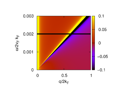
Figure 3: (Color online) $(a)$ Color plot of the dimensionless quantity $\rho(E_{F})\>{V}(q,\omega)$ for $k_{F}=1\;\text{nm}^{-1}$ in the $q/\omega$ plane ($\alpha=35eV$). The horizontal black line at $\omega/v_{F}k_{F}=0.002$ marks a cross section of the plot that is drawn separately in the panel $(b)$.

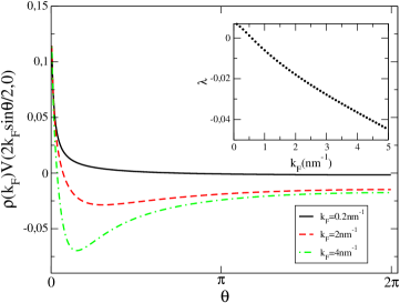
Figure 4: Plot of the dimensionless product $\rho\left(E_{F}\right)\>V(2k_{F}\sin\theta/2,0)$ of Eq.(20) versus the scattering angle $\theta$ for various values of $k_{F}$ ($\alpha=35eV$).The inset shows the dependence of the pairing coupling strength $\lambda$ versus $k_{F}$

In the final stages of preparing this manuscript, we became aware of Ref. Das Sarma and Li, 2013 which is related to this work. In this paper the estimate of the pairing strength $\lambda$ of Eq. (22) is about one order of magnitude larger than what found here, thus leading to a different conclusion about the possibility of induced surface superconductivity.

Acknowledgments: One of us (V.P.) acknowledges useful discussions with E. Cappelluti and P. Lucignano. This work was done with financial support from FP7/2007-2013 under the grant N. 264098 - MAMA (Multifunctioned Advanced Materials and Nanoscale Phenomena), MIUR-Italy through Prin-Project 2009 ”Nanowire high critical temperature superconductor field-effect devices”, as well as the Helmholtz Virtual Insitute ”New States of Matter”. V.P. and F. G. acknowledge financial support from MINECO, Spain, through grant FIS2011-23713, and the European Union, through grant 290846.

Appendix A Matrix elements of the e-ph interaction

The matrix elements of the e-ph interaction appearing in Eq(2) require that the contraction of the strain tensor $(\partial_{i}U_{j}+\partial_{j}U_{i})/2$ with appropriate $4\times 4$ matrix $A_{ij}$ is invariant with respect to the symmetry operations of the little groups Lyubarskii (1960) preserving the wave vectors of the electrons and phonons, respectively. Long-wavelength phonons have momenta close to the $\Gamma$ point and thus the little group for a generic $\vec{q}$ is the space group of the crystal. In TIs as Bi₂Se₃ the surface states are close to the $\Gamma$ point, as well, so that the little group of the surface states is again the space group of the lattice, as for the phonons. In the case of Bi₂Se₃ the space group is $G=\{C_{6},\mathcal{I},\mathcal{T}\}$, where $\mathcal{I}$ is the space inversion and $\mathcal{T}$ is the time reversal. Let the $orbital\otimes spin$ space be addressed by the Pauli matrices $\vec{\tau}$ and $\vec{\sigma}$ , respectively.The Dirac matrices are $\gamma_{0}=i\mathbb{I}\otimes\tau_{z},\>\gamma_{i}=\sigma_{i}\otimes\tau_{x}\>(i=1,..3)$, where $\mathcal{I}$ is the identity matrix. In the first and the fourth column of Table 1 we enumerate all the matrices $\Gamma_{\nu}$ that can be built in the given space. Besides the identity and $\gamma_{5}=i\alpha_{0}\gamma_{1}\gamma_{2}\gamma_{3}=-\mathbb{I}\otimes\tau_{y}$ there are the four matrices $\gamma_{0}\gamma_{5}=\mathbb{I}\otimes\tau_{x},\>\gamma_{i}\gamma_{5}=-i\sigma_{i}\otimes\tau_{z}$ and the six matrices $\Sigma_{\mu\nu}=i/2[\gamma_{\mu},\gamma_{\nu}]$ given by

$$\begin{split}\Sigma_{0i}&=-i\sigma_{i}\otimes\tau_{y}\\ \Sigma_{ij}&=\epsilon_{ijk}\sigma_{k}\otimes\mathbb{I}\end{split}$$ (23)

(with $i<j$). These 15 matrices, plus the identity matrix, make a basis in the space of $4\times 4$ matrices $\{\Gamma_{i}\}$ explicitly written in table 1. The label $Y$ in the $C_{6}$ and $\mathcal{T}$ columns of the Table marks the matrices which are conserved by the symmetry operations $C_{6}$ or $\mathcal{T}$.

Matrix	$C_{6}$	$\mathcal{T}$	Matrix	$C_{6}$	$\mathcal{T}$
$\mathbb{I}$	Y	Y	i$\gamma_{2}\gamma_{5}$
$\gamma_{0}$	Y	Y	i$\gamma_{3}\gamma_{5}$	Y
$\gamma_{1}$			i$\Sigma_{01}$		Y
$\gamma_{2}$			i$\Sigma_{02}$		Y
$\gamma_{3}$	Y		i$\Sigma_{03}$	Y	Y
$\gamma_{5}$	Y		$\Sigma_{12}$	Y
$\gamma_{0}\gamma_{5}$	Y	Y	$\Sigma_{13}$
i$\gamma_{1}\gamma_{5}$			$\Sigma_{23}$

Table 1: Basis in the space of $4\times 4$ matrices.

From table 1 it is possible to extract 4 spacially constant vectors

	TR	I
$\boldsymbol{a}=(\gamma_{1},\gamma_{2},\gamma_{3})$	-1	-1
$\boldsymbol{b}=(\Sigma_{23},\Sigma_{31},\Sigma_{12})$	-1	+1
$\boldsymbol{p}=(i\Sigma_{01},i\Sigma_{02},i\Sigma_{03})$	+1	-1
$\boldsymbol{b}^{\prime}=(i\gamma_{1}\gamma_{5},i\gamma_{2}\gamma_{5},i\gamma_{3}\gamma_{5})$	-1	+1

which give rise to seven second rank tensors conserving time reversal: $a_{i}a_{j},b_{i}b_{j},b^{\prime}_{i}b^{\prime}_{j},p_{i}p_{j},a_{i}b_{j},b_{i}b^{\prime}_{j},a_{i}b^{\prime}_{j}$. The tensors $a_{i}b_{j}$ and $a_{i}b^{\prime}_{j}$ must be dropped because they break inversion symmetry. The first surviving tensors are identical, since

$$\begin{split}\Sigma_{\mu\nu}\Sigma_{\mu\eta}&=\gamma_{\nu}\gamma_{\eta}\\ (i\gamma_{\mu}\gamma_{5})(i\gamma_{\nu}\gamma_{5})&=\gamma_{\mu}\gamma_{\nu}\end{split}$$ (24)

so that we are left just with the two independent bilinears:

$$\begin{split}A_{ij}\equiv a_{i}a_{j}&=(\sigma_{i}\otimes\tau_{x})(\sigma_{j}\otimes\tau_{x})=\delta_{ij}\mathbb{I}\otimes\mathbb{I}+i\epsilon_{ijk}\sigma_{k}\otimes\mathbb{I}\\ B_{ij}\equiv b_{i}b^{\prime}_{j}&=(\sigma_{i}\otimes\mathbb{I})(\sigma_{j}\otimes\tau_{z})=\delta_{ij}\mathbb{I}\otimes\tau_{z}+i\epsilon_{ijk}\sigma_{k}\otimes\tau_{z}\>.\end{split}$$ (25)

Contraction of each of these matrices with the symmetric strain tensor cancels the antisymmetric part of both bilinears. We ignore the perturbative matrix elements arising from $B_{ij}$ because they would induce changes in the bulk gap of the material and we get the final result of Eq.(2) with $A_{ij}=\delta_{ij}\mathbb{I}\otimes\mathbb{I}$.

Appendix B Conditions for the existence of the Rayleigh mode in a slab geometry

Question arises whether a surface layer with softer elastic constants, attached to a more rigid background, still supports the Rayleigh mode. Here below we answer positively to this question by discussing the existence conditions within linear elasticity theory in the limit of a thin surface layer (hereafter defined ”the slab”).

Let us consider a slab with elastic constants $\lambda_{1},\mu_{1}$, with thickness $h$, rigidly attached to a semi-infinite medium occupying the region $z<0$, with constants $\lambda_{2},\mu_{2}$ . Both the slab and the bulk are considered homogeneous elastic media described by the stress tensor

$$\sigma_{ij}=\frac{E}{1+\sigma}\left(u_{ij}+\frac{\sigma}{1-2\sigma}u_{ll}\delta_{ij}\right)=2\rho[c_{t}^{2}u_{ij}+(c_{l}^{2}-2c_{t}^{2})u_{ll}\delta_{ij}].$$ (26)

Boundary conditions are given by

• free surface condition at $z=h$

  $$\sigma_{1}\cdot n_{z}|_{z=h}=0$$ (27)

• continuity of stress at $z=0$

  $$\sigma_{1}\cdot n_{z}|_{z=0}=\sigma_{2}\cdot n_{z}|_{z=0}$$ (28)

• continuity of displacement at $z=0$

  $$u_{1}|_{z=0}=u_{2}|_{z=0}.$$ (29)

In the geometry described above two different polarization are possible for surface phonons: Rayleigh modes, polarized in the $xz$ plane, and the Love waves, polarized in the $xy$ plane. We only consider the Rayleigh mode here, as a discussion on Love can be found for example in Ref.Pujol (2003).

To write the general Ansatz on the displacement vector we introduce the function $\phi(\textbf{r})$ and the vector function $\boldsymbol{\chi}(\textbf{r})$, so that the longitudinal and the transverse part of u read

$$\begin{split}\textbf{u}_{L}(\textbf{r})&=\nabla\phi\\ \textbf{u}_{T}(\textbf{r})&=\nabla\times\boldsymbol{\chi}.\end{split}$$ (30)

The function $\phi$ and each component of $\boldsymbol{\chi}$ satisfy the wave equation with velocity of propagation $c_{l}$ and $c_{t}$ respectively. The most general form of these functions giving surface waves polarized in the $xz$ plane of the slab are

$$\begin{split}\phi&=(A\sinh\lambda_{l}z+B\cosh\lambda_{l}z)e^{i(kx-\omega t)}\\ \boldsymbol{\chi}&=\hat{e}_{y}(C\sinh\lambda_{t}z+D\cosh\lambda_{t}z)e^{i(kx-\omega t)}.\end{split}$$ (31)

Correspondingly, the functions $\phi$ and $\boldsymbol{\chi}$ for the background are

$$\begin{split}\phi&=Ee^{\lambda_{l}z}e^{i(kx-\omega t)}\\ \boldsymbol{\chi}&=\hat{e}_{y}Fe^{\lambda_{t}z}e^{i(kx-\omega t)},\end{split}$$ (32)

The solution of this system of six equations in the six unknowns given by Eqs. (27), (28) and (29) exists provided the determinant of the coefficient matrix vanishes. In principle the vanishing of the determinant defines the dispersion relation for the surface waves. In this case, the secular equation will be of the 12th degree, and some simplification is needed to understand the physics in a faster and clearer way. The first step is to consider a thin slab, whose thickness is negligible compared to the background. In this case, one can take only the zero-th approximation for displacement vector in the slab. This approximation is possible since, in the slab, there is a combination of hyperbolic functions in the definition of u. In this approximation the system becomes

$$\begin{split}2ik\lambda_{l1}A-(k^{2}+\lambda_{t}^{2})D&=0\\ [c_{l1}^{2}\lambda_{l1}^{2}-(c_{l1}^{2}-2c_{t1}^{2})k^{2}]B+2ik\lambda_{t1}c_{t1}^{2}C&=0\\ [2ik\lambda_{l2}E-(k^{2}+\lambda_{t2}^{2})F]&=0\\ [c_{l2}^{2}\lambda_{l2}^{2}-(c_{l2}^{2}-2c_{t2}^{2})k^{2}]E+2ik\lambda_{t1}c_{t1}^{2}F&=0\\ ikB-\lambda_{t1}C&=ikE-\lambda_{t2}F\\ \lambda_{l1}A+ikD&=\lambda_{l2}E+ikF.\end{split}$$ (33)

The structure of system (33) enlightens the physics of surface states of this composite material. The third and the fourth equations for $E$ and $F$ above coincide with the system defining Rayleigh waves at the interface between the slab and the backgroundLandau and Lifshitz (1975). Given a non trivial solution for granted, the penetration of this mode leads to the definition of Rayleigh waves at the interface between the slab and the vacuum too obtained from the remaining equations.

In particular we are left with the inhomogeneous system of four equations in the four unknowns A,B,C,D:

$$\begin{split}2ik\lambda_{l1}A-(k^{2}+\lambda_{t}^{2})D&=0\\ [c_{l1}^{2}\lambda_{l1}^{2}-(c_{l1}^{2}-2c_{t1}^{2})k^{2}]B+2ik\lambda_{t1}c_{t1}^{2}C&=0\\ ikB-\lambda_{t1}C&=M_{1}\\ \lambda_{l1}A+ikD&=M_{2},\end{split}$$ (34)

where $M_{1}$ and $M_{2}$ are assumed to be given quantities, once the homogeneous system for $E,F$ has been solved. They involve the ratio between the velocity of Rayleigh waves $c_{R}$ and the transverse velocity in the bulk, $\xi_{2}=c_{R}/c_{t2}$. In this case, the determinant ${\cal{D}}$ of the matrix for the coefficients $A,B,C,D$ has to be different from zero

$${\cal{D}}=c_{l1}^{2}\lambda_{l1}\lambda_{t1}(k^{2}-\lambda_{t1}^{2})(\lambda_{l1}^{2}-k^{2}),$$ (35)

provided that or, using the definition of the $\lambda$’s given in the main text $\lambda_{l}=\sqrt{1-c_{R}/c_{l}}$ and $\lambda_{t}=\sqrt{1-c_{R}/c_{t}}$

$${\cal{D}}=-c_{l1}^{2}\sqrt{1-\gamma^{2}\xi^{2}}\sqrt{1-\xi^{2}}k^{6}\xi^{4}\gamma^{2}.$$ (36)

$$\xi_{2}=\frac{c_{R}}{c_{t2}}=\frac{c_{R}}{c_{t1}}\frac{c_{t1}}{c_{t2}}=\xi_{1}\>\frac{c_{t1}}{c_{t2}}.$$ (37)

The determinant $\mathcal{D}$ can be non zero provided $0\neq\xi_{1}<1$ and therefore the system of Eq.(34) has a non trivial solution.There are some restrictions, though, on the elastic parameters in the two materials, stemming from $\xi_{1}<1$:

$$\xi_{2}\frac{c_{t2}}{c_{t1}}<1\Rightarrow\frac{c_{t2}}{c_{t1}}<\frac{1}{\xi_{2}}.$$

References

- Zhang et al. (2009) H. Zhang, C.-X. Liu, X.-L. Qi, X. Dai, Z. Fang, and S.-C. Zhang, Nature Phys. 5, 438 (2009).
- Hasan and Kane (2010) M. Z. Hasan and C. L. Kane, Rev. Mod. Phys. 82, 3045 (2010).
- Giraud and Egger (2011) S. Giraud and R. Egger, Phys. Rev. B 83, 245322 (2011).
- Zhu et al. (2011) X. Zhu, L. Santos, R. Sankar, S. Chikara, C. Howard, F. C. Chou, C. Chamon, and M. El-Batanouny, Phys. Rev. Lett. 107, 186102 (2011).
- Zhu et al. (2012) X. Zhu, L. Santos, C. Howard, R. Sankar, F. C. Chou, C. Chamon, and M. El-Batanouny, Phys. Rev. Lett. 108, 185501 (2012).
- Pan et al. (2012) Z.-H. Pan, A. V. Fedorov, D. Gardner, Y. S. Lee, S. Chu, and T. Valla, Phys. Rev. Lett. 108, 187001 (2012).
- V. Sandomirsky and Schlesinger (2001) R. L. V. Sandomirsky, A. V. Butenko and Y. Schlesinger, J. Appl. Phys. 90, 2370 (2001).
- Greenaway and Harbeke (1965) D. Greenaway and G. Harbeke, J. Phys. Chem. Solids 26, 1585 (1965).
- Ezawa (1971) H. Ezawa, Ann. Phys. 67, 438 (1971).
- Landau and Lifshitz (1975) L. D. Landau and E. M. Lifshitz, Theory of Elasticity (Pergamon Press, 1975).
- Huang and Kaviany (2008) B.-L. Huang and M. Kaviany, Phys. Rev. B 77, 125209 (2008).
- Mahan (1990) G. D. Mahan, Many-Particle Physics (Plenum Press, 1990).
- Park et al. (2008) C.-H. Park, L. Yang, Y.-W. Son, M. L. Cohen, and S. G. Louie, Phys. Rev. Lett. 101, 126804 (2008).
- Guinea and Low (2010) F. Guinea and T. Low, Phil.T. Roy. Soc. A 368, 5391 (2010).
- Yankowitz et al. (2012) M. Yankowitz, J. Xue, D. Cormode, J. D. Sanchez-Yamagishi, K. Watanabe, T. Taniguchi, P. Jarillo-Herrero, P. Jacquod, and B. J. LeRoy, Nat. Phys. 8, 382 (2012).
- Tanaka et al. (2012) Y. Tanaka, K. Nakayama, S. Souma, T. Sato, N. Xu, P. Zhang, P. Richard, H. Ding, Y. Suzuki, P. Das, Phys. Rev. B 85, 125111 (2012).
- Analytis et al. (2010) J. G. Analytis, R. D. McDonald, S. C. Riggs, J.-H. Chu, G. S. Boebinger, and I. R. Fisher, Nat. Phys. 6, 960 (2010).
- Das Sarma and Li (2013) S. Das Sarma and Q. Li (2013), eprint cond-mat/1305.3605.
- Lyubarskii (1960) G. Lyubarskii, The Application of Group Theory (Pergamon Press, 1960).
- Pujol (2003) J. Pujol, Elastic Wave Propagation and Generation in Seismology (Cambridge, 2003).