Comparison of H i and optical redshifts of galaxies - The impact of redshift uncertainties on spectral line stacking

Abstract

Accurate optical redshifts will be critical for spectral co-adding techniques used to extract detections from below the noise level in ongoing and upcoming surveys for H i, which will extend our current understanding of gas reservoirs in galaxies to lower column densities and higher redshifts. We have used existing, high quality optical and radio data from the SDSS and ALFALFA surveys to investigate the relationship between redshifts derived from optical spectroscopy and neutral hydrogen (H i) spectral line observations. We find that the two redshift measurements agree well, with a negligible systematic offset and a small distribution width. Employing simple simulations, we determine how the width of an ideal stacked H i profile depends on these redshift offsets, as well as larger redshift errors more appropriate for high redshift galaxy surveys. The width of the stacked profile is dominated by the width distribution of the input individual profiles when the redshift errors are less than the median width of the input profiles, and only when the redshift errors become large, $\sim$150 km s^-1, do they significantly affect the width of the stacked profile. This redshift accuracy can be achieved with moderate resolution optical spectra. We provide guidelines for the number of spectra required for stacking to reach a specified mass sensitivity, given telescope and survey parameters, which will be useful for planning optical spectroscopy observing campaigns to supplement the radio data.

1 Introduction

Measurements of the neutral hydrogen (H i) gas content of galaxies as a function of redshift are critical to our understanding of galaxy formation and evolution. In the local Universe, large area surveys such as the H i Parkes All-Sky Survey (HIPASS, Barnes et al. 2001, Meyer et al. 2004) and the Arecibo Legacy Fast ALFA survey (ALFALFA, Giovanelli et al. 2005) have evaluated metrics such as the H i mass function and the local H i matter density ($\Omega_{HI}$) with increasing accuracy (see, for example Zwaan et al. 2005, Martin et al. 2010). Combined with complementary multi-wavelength photometry and spectroscopy, these surveys have greatly expanded our understanding of the gaseous and stellar components of local galaxies as a function of environment, and provide a $z=0$ reference for cosmological simulations that incorporate gas physics into galaxy formation.

A galaxy’s H i gas content serves as a reservoir of fuel for future star formation. Surveys of the stellar content of galaxies show that the star formation rate decreases by an order of magnitude from $z\sim 1$ to the present day (Madau, Pozzetti, & Dickinson 1998, Hopkins & Beacom 2006, for example), however, little is known of the H i content of galaxies in this epoch. Simulations by Obreschkow et al. (2009) and Lagos et al. (2011) predict the evolution in the size, velocity profile, Tully-Fisher relation, and H i mass function of H i disks as a function of redshift. However, the bandwidth accessible to existing radio telescopes, combined with the intrinsically weak signal from the 21 cm line of neutral hydrogen, have made comprehensive surveys of H i emission at redshifts beyond $z>0.1$ technically challenging, or prohibitively expensive in terms of telescope time.

Observations seeking to detect H i in emission at intermediate redshift have employed a number of different strategies. Catinella et al. (2008) used the Arecibo Observatory to detect 10 massive field galaxies out to a redshift of $z=0.25$. While single dish telescopes are very sensitive, they lack the spatial resolution to resolve individual galaxies at all but the lowest redshifts.

The high sensitivity of large single dish radio telescopes is an advantage to those interested in studying large scale baryon acoustic oscillations: Chang et al. (2010) report the detection of H i emission at a redshift of $z=0.8$ by cross correlating the weak radio signal from the Robert C. Byrd Green Bank Telescope with a map of the large scale structure known from optical spectroscopic observations.

Interferometric observations, with higher spatial resolution, are able to resolve individual galaxies within large-scale structures. Utilising available bandwidths, observations have successfully targeted narrow redshift ranges around known galaxy clusters. In $\sim$2300 hours of observations with the Westerbork Synthesis Radio Telescope (WSRT), the Blind Ultra-Deep H i Environmental Survey has detected more than 150 galaxies in Abell 963 and Abell 2192 at $z=0.206$ and $z=0.188$, respectively (Jaffé et al., 2013).

Increased computing power and improvements in receiver technology are advancing the field of radio astronomy by enabling larger volumes to be surveyed to greater depth in vastly reduced time. This progress enables radio surveys to become competitive with observations at other wavelengths in terms of both survey area and accessible redshift.

Recent upgrades to the Karl G. Jansky Very Large Array (VLA) mean is now possible to observe H i over a continuous redshift range from $0<z<0.45$. The CHILES (COSMOS H i Large Extragalactic Survey) collaboration has demonstrated the feasibility of such a survey in a pilot project spanning $0<z<0.193$ (Fernández et al., 2013). APERture Tile in Focus (APERTIF), a focal-plane array system, will increase the field of view of the WSRT, allowing faster mapping of large areas of sky while measuring the H i content of galaxies out to $z=0.3$ (Verheijen et al., 2008).

The upgrades to existing facilities serve as critical testbeds for future facilities such as South Africa’s MeerKAT (Jonas 2009) and the Australian Square Kilometre Array Pathfinder (ASKAP, Johnston et al. 2008), which themselves are to be precursor instruments for the international Square Kilometre Array (SKA) Telescope. The SKA and the precursors will enable observations of neutral hydrogen over cosmologically significant ranges of redshift and to lower column densities than are possible with existing instrumentation.

Several surveys, such as Looking at the Distant Universe with the MeerKAT Array (LADUMA, Holwerda et al. 2012), Deep Investigation of Neutral Gas Origins (DINGO), Widefield ASKAP L-band Legacy All-sky Blind surveY (WALLABY) and deep APERTIF WSRT surveys are in advanced planning stages and are set to begin within the next few years. These surveys, requiring many thousands of hours of observing time, aim to explore new parameter space and will operate at the limits of the capabilities of the survey telescopes. However, even with the unprecedented sensitivity of these instruments, direct H i detections at moderate ($z\sim 0.5$) redshifts will be rare due to the intrinsic weakness of the emission.

In order to extend the range of measurements to lower H i column densities and higher redshifts, while keeping observation times practical, techniques for extracting information from datasets without statistical detections, such as spectral stacking, are being investigated. These techniques will be critical for the success of the above mentioned surveys, particularly the projects aiming to study the neutral hydrogen content of galaxies at $z\sim 1$.

1.1 H i Spectral Stacking

Stacking a large number of non-detections in order to build up a single detection and recover the statistical properties of the contributing ensemble of objects has long been used, primarily in imaging data (Dunne et al. 2009, Karim et al. 2011). The spectral dimension of a radio cube allows us to stack not only images but spectra as well. For the current work, we are only interested in detecting H i 21cm line emission from neutral hydrogen, not continuum emission resulting from star formation or active galactic nucleus (AGN) activity.

Radio spectral stacking relies on information from supplementary observations, usually optical imaging and spectroscopy, to provide the sky positions and redshifts of a collection of galaxies. The corresponding radio data-cube also contains the H i emission from the known galaxies, even if they are formally undetected. Spectra are extracted from the cube at the locations of the known galaxies, shifted to the rest-frame of each galaxy, and co-added, or stacked, to build up an average detection from many non-detections. Section 3 in Fabello et al. (2011) contains a comprehensive description of the stacking procedure.

In order to reach lower H i mass sensitivity in less observing time, Chengalur, Braun, & Wieringa (2001) undertook a deliberately shallow observation of Abell 3128 ($z=0.06$) to test H i spectral line stacking. This technique has also been successfully employed by a number of groups to extend H i studies to higher redshifts (Lah et al. 2007, Lah et al. 2009) and lower H i content (Fabello et al. 2011, Delhaize et al. 2013). Khandai et al. (2011) employ N-body simulations incorporating H i to investigate the putative stacked signal at $z\sim 1$ with encouraging results.

The primary assumption behind using optical redshifts for H i spectral stacking is that the redshift determined from the optical spectra is the same as that which would be determined from the H i data, if it could be detected. This point is either assumed to be approximately true with any differences averaging to zero (Fabello et al., 2011), or the differences are sufficiently small that they can largely be ignored (Lah et al., 2007). For galaxies undergoing major mergers, or galaxies in overdense environments, the stars and gas can have very different kinematic profiles (Haynes, Giovanelli, & Kent 2007, Chung et al. 2009), and the assumption of identical optical and H i redshifts will break down.

The success of stacking also depends on the quality of the optical (or other supplementary) astrometry and spectroscopy in particular. Accurate redshifts of the galaxies are required in order to properly align the non-detected galaxies in the spectral dimension. If the errors on the measured redshifts are large, the H i profiles will no longer be aligned and the stacked profile will be smeared out.

The stacked signal is also sensitive to the noise properties of the radio data. For a signal buried in Gaussian noise, stacking will increase the flux in the signal linearly with the number of spectra contributing to the stack ($n_{spec}$), but the noise increases only as the square root of the number of spectra, thus the signal-to-noise ratio (S/N) increases as $\sqrt{n_{spec}}$. This is not the case for non-Gaussian noise.

The purpose of this work is to determine how closely redshifts derived from optical spectroscopy relate to those measured from H i profiles using a sample of galaxies that are detected at high significance in both optical and radio data. We are particularly interested in determining the width of the distribution of the redshift differences, as well as any systematic offset that may be present. We compare a number of methods of measuring the optical redshift to assess whether particular measurements have advantages over others. Finally, we employ simple simulations to determine the effect this redshift difference has on a putative stacked profile, and finish with recommendations of minimum data quality requirements for future stacking endeavours.

The outline of the paper is as follows. Section 2 describes the data used for the study, and Section 3 compares the redshifts derived from optical and radio observations of the same galaxies. Section 4 introduces the simple stacking simulation we employ to investigate redshift offsets between the optical and radio observations, Section 5 describes the results of our simulations and Section 6 puts the results in the context of upcoming surveys. Our conclusions are given in Section 7.

2 Input H i and Optical Data

The H i data come from the ALFALFA survey (Giovanelli et al. 2005, Giovanelli et al. 2005, and Giovanelli et al. 2007), specifically the $\alpha$.40 H i source catalog from Haynes et al. (2011). The parameters of most interest for the present study are the measured H i recession velocity and the velocity width of the H i line profile measured at the 50 per cent level of the peak, $W_{50}$.

The optical photometry and spectroscopy are from the Sloan Digital Sky Survey (SDSS, York et al. 2000) Data Release 7 (DR7, Abazajian et al. 2009). The ALFALFA team has carefully crossmatched the $\alpha$.40 H i detections to the SDSS database to determine the optical counterpart for each. We include only the SDSS matches that also have an optical spectrum, resulting in 9974 matches. From this crossmatch, the SDSS ObjID and SpecObjID identifiers are known, and further information from the SDSS database can be extracted.

Flags from the crossmatch indicate a secure counterpart, or some confusion regarding the photometric or spectroscopic data. We only use galaxies with an unambiguous optical counterpart possessing an SDSS spectrum from the morphological centre of the galaxy to create a clean starting sample, reducing the sample size to 9578.

The sample is further reduced by imposing $v_{sys}$$\leq 15\,000$ km s^-1 to cut out H i data heavily affected by radio frequency interference (RFI, Martin et al. 2010). Additionally, galaxies with an active nucleus and broad emission lines, identified with SDSS spectral classification ‘AGN’, are removed, leaving 8923 galaxies.

The quality of the H i detection determined by visual inspection of individual H i spectra is set as a flag within the ALFALFA catalogue. Code 1 implies a reliable detection of high S/N, whereas Code 2 detections generally have lower S/N but a plausible optical counterpart lending support to the detection. Imposing a straight S/N cut results in a similar, but not identical, separation of the two categories.

The Code 1–2 designation is based on the quality of the H i spectra, and is not a quantity intrinsic to the H i properties. We therefore exclude the Code 2 ALFALFA galaxies from the sample, as we aim to investigate the offset between optical and H i velocities, independent of problems arising from their measurement. This final restriction leaves 6419 galaxies, and we refer to this subset of ALFALFA galaxies with secure optical counterparts and high confidence H i parameters as the ALFALFA–SDSS sample.

3 H i vs Optical Redshifts

We wish to compare the redshifts, or equivalently, the recession velocities, of the ALFALFA–SDSS galaxies as determined from the H i and the optical spectra. First, we investigate each of the optical and H i measures separately, to gain confidence in their reliability. Throughout, we convert between redshift and recession velocity with $v=cz$, where $c=299792.458$ km s^-1, as do Haynes et al. (2011) for the H i velocity measurements. Both the SDSS and the ALFALFA velocities are set to the heliocentric reference frame.

3.1 Spectroscopic Reliability

HIPASS (Barnes et al. 2001, Meyer et al. 2004), the Equatorial Survey (ES, Garcia-Appadoo et al. 2009) subset, and the Northern HIPASS catalogue (NHICAT, Wong et al. 2006) serve as an independent check of the reliability of the recession velocities derived for the ALFALFA galaxies. There are 142 unambiguous matches between HIPASS ES and NHICAT and ALFALFA, as determined from inspection of the SDSS imaging, of which 109 are matches with ALFALFA optical counterpart flag ‘I’, indicating a single optical counterpart has been identified. The HIPASS observations are not as sensitive as ALFALFA, so only the most H i-rich galaxies appear in the overlapping sample, and the S/N of the ALFALFA H i detections is high. The spectral resolution of HIPASS, at 18 km s^-1, is also lower than the 11 km s^-1 resolution of ALFALFA.

As seen in Fig. 1, the measured systemic velocities of galaxies common to both ALFALFA and HIPASS correspond very well. There are a few large velocity difference outliers, and visual inspection of the SDSS images shows that there is always another galaxy within the larger HIPASS beam that could be causing confusion.

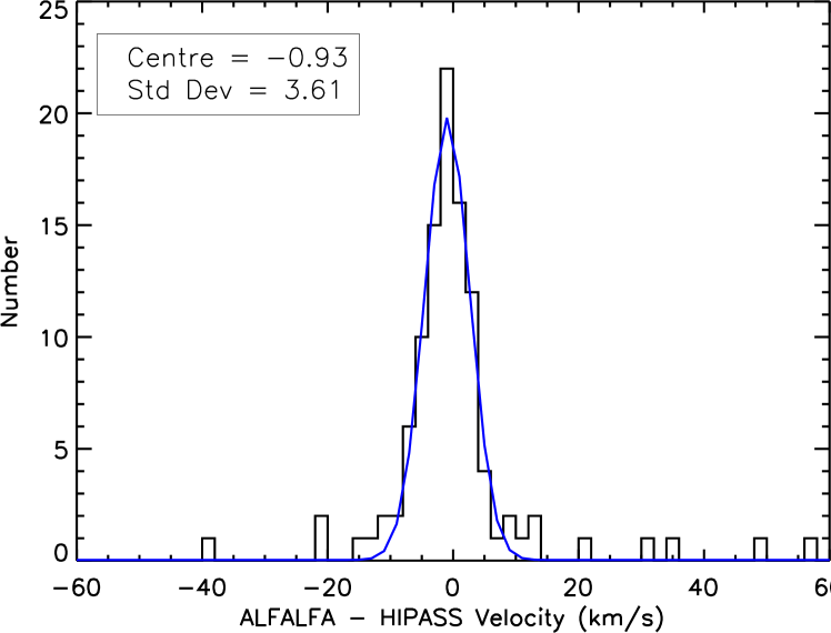
Figure 1: The measured recession velocity differences for ALFALFA galaxies matched to HIPASS ES and NHICAT to determine the repeatability of the ALFALFA redshifts. The centre and the standard deviation of the Guassian fit to the distribution are given in the plot legend.

A similar exercise can be done for the optical redshifts, as a number of galaxies have repeat observations, i.e. two or more spectra at the same sky position observed on different nights. There are 240 ALFALFA galaxies with repeat observations, with the difference in recession velocities derived from each pair of spectra shown in Fig. 2. The width of this distribution, $\sim$10 km s^-1, is much smaller than the 60 km s^-1 error quoted by the SDSS data releases, possibly because the ALFALFA–SDSS galaxies of interest here are all at $z\leq 0.05$ and are generally bright. Therefore, we conclude that, at least for the H i-rich and optically bright galaxies, we can treat both the H i and the optical recession velocities as highly reproducable.

Figure 2: The velocity difference for the 240 galaxies in ALFALFA with more than one SDSS spectrum at the same position on the sky (i.e. repeat observations). The centre and the standard deviation of the Guassian fit to the distribution are given in the plot legend.

3.2 Optical Redshift Measurements

The SDSS provides several redshift measurements for each spectrum derived via independent methods, stored in different tables in the Catalog Archive Server (CAS) database. Since we are interested in the differences between radio and optical redshift determinations, we need to ensure that we are using the best measurements available.

For each spectrum, the redshifts derived from fitting the emission lines are stored in the ELRedshift table, with an associated confidence. The SpecLine table stores the fit parameters to the individual measured emission lines used to derive the ELRedshift result. Single Gaussians are fit to individual features, which become inappropriate for non-Gaussian shaped features.

Alternatively, a cross-correlation of spectral templates to the spectra is also performed, masking out emission features and using only absorption features. The resulting redshift and its error is stored in the XCRedshift table. The redshift from the SpecObj table, simply listed with the variable name $z$, is the redshift determined from the emission lines or cross-correlation method, whichever has the higher confidence. Fig. 3 compares the recession velocity from the SpecObj $z$ and that from the H i measurements for the ALFALFA–SDSS galaxies. The distribution is approximately Gaussian, and the resulting fit is offset from zero by -6.9 km s^-1 and has width $\sigma=19.9$ km s^-1. This distribution is similar to that found by Toribio et al. (2011), who also compared optical and H i recession velocities for ALFALFA galaxies with SDSS spectroscopy, and found a distribution with dispersion $\sim 35$ km s^-1. The reduced width found here is due to our exclusion of Code 2 ALFALFA detections and requirement that the SDSS spectrum be centred on the galaxy. There are non-Gaussian wings of the distribution in Fig. 3, with non-negligible numbers of galaxies having velocity differences $>|40|$ km s^-1. These are discussed further in Section 3.3.

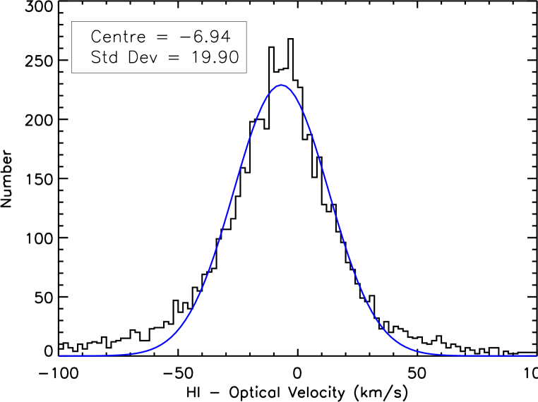
Figure 3: The difference between the velocity derived from the H i and that from the SDSS SpecObj $z$, based on the ALFALFA–SDSS galaxies. The centre and the standard deviation of the Gaussian fit are given in the plot legend.

There is a known velocity offset of 7.3 km s^-1 of the reported SpecObj $z$ redshifts from the SDSS, in the sense that the stated values are too low (Adelman-McCarthy et al., 2008). The origin of the offset is still unknown, but it persists in the DR7 data. If a correction is applied to the redshifts in Fig. 3, the offset from zero becomes -14.2 km s^-1. This offset is corrected in the sppParams table, which uses the Spectro Parameter Pipeline (spp) processing instead of the spectro1d pipeline which results in the SpecObj $z$ value.

Lastly, a collaboration of researchers at the Max Planck Institute for Astrophysics (MPA) and the Johns Hopkins University (JHU) have produced the MPA-JHU value-added galaxy catalogue (hereinafter referred to as the MPA–JHU catalogue), which provides spectral properties derived from an independent analysis of the SDSS DR7 galaxy spectra. Within the MPA–JHU catalogue, a stellar population model is fit to the galaxy continuum to properly account for absorption features, which can be significant in some cases. Further details of the fitting procedure can be found in Tremonti et al. (2004) and Brinchmann et al. (2004), or at the website hosting the catalogues. The redshifts from the sppParams table agree very well with those from the MPA-JHU catalogue.

The comparison of MPA–JHU catalogue and H i velocities is shown in Fig. 4. The distribution is much narrower than that in Fig. 3, and the offset from zero is greatly reduced. Fitting with two Gaussians produces a very good fit to both the core and the wings of the distribution. The two Gaussians may imply two distinct populations contributing to the total sample, and it allows for a simple and useful parametrization of the H i-optical velocity offsets. As the MPA–JHU catalogue does not suffer from the 7.3 km s^-1 offset, and there are additional useful measurements within the MPA–JHU catalogue, we use these values for the optical redshifts of the ALFALFA–SDSS galaxies.

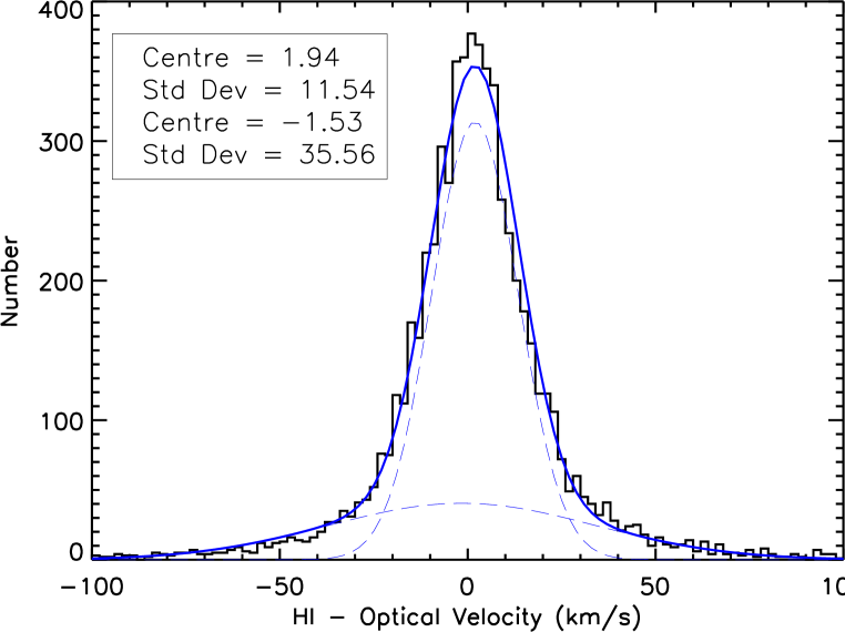
Figure 4: The difference between the velocity derived from the H i and that from the JHU–MPA reprocessed data. The centres and standard deviations of the two Gaussian fits (blue dashed lines) are given in the legend. The blue solid line is the sum of the two individual curves.

3.3 Velocity Outliers

Fig. 4 shows that the optical and the H i velocities do not match exactly, and there is a significant population of galaxies with velocity offsets $>|40|$ km s^-1, which marks where the distribution is entirely composed of objects in the broader distribution. We wish to know if there is any observable property that can be exploited to reduce the width of the distribution or reduce the number of velocity outliers.

Eight per cent of the ALFALFA–SDSS galaxies have H i-optical velocity differences $>|40|$ km s^-1. We investigated several parameters in an attempt to isolate the outliers, including the width of the H i profile (measured as $W_{50}$), H i flux, H i S/N, H i mass and the errors associated with each of these measures, the optical $u-r$ colour, optical galaxy orientation, and optical spectrum S/N. While there is tentative evidence that the velocity outliers have widths $W_{50}$ greater than the median width of 150 km s^-1, from visual inspection of the H i and optical spectra, there is no obvious trend for any of these parameters to preferentially select velocity outliers.

Nearly ten per cent of the ALFALFA galaxies have publicly available H i spectra accessible online, and more will become available as the H i archive is updated. Visual inspection of the outlier H i profiles combined with the optical images from SDSS and DSS2 can help determine the causes of the large offset between the H i and optical velocities. We find a number of factors which may be responsible for large H i–optical offsets:

• Asymmetric H i profiles – The majority of cases fall within this category. The intrinsic H i profile may be severely aysmmetric, leaving one side undetected. Alternatively, the emission from the systemic velocity of the galaxy may only be at the same level as the noise, making it difficult to recognize two peaks in the spectrum belonging to the same H i profile.

• Clearly disturbed, interacting systems – High S/N H i emission from a tidal tail or infalling gas contributes to the width of the H i profile. These are likely outliers because the systemic velocity of the galaxy is determined by the midpoint of the $W_{50}$ profile, whereas the optical redshift is determined from a fibre on the morphological centre of the galaxy.

• Blended H i profiles – More than one galaxy in the Arecibo beam, with H i profiles overlapping in velocity space, but the galaxies are not necessarily interacting. The optical spectrum will generally only measure the recession velocity for one of the galaxies, whereas the H i profile may have contributions from several components.

• Mis-identified H i profiles – These are extremely rare among the Code 1 sources, and may be due to difficult baseline subtraction, a portion of the data having lower weight, or the presence of RFI.

• Absorption line spectrum – A number of galaxies have significant reservoirs of H i but do not show emission lines in their optical spectrum. We will discuss in Section 3.4 that optical redshift measurements derived from absorption features are more uncertain.

In the context of H i stacking, only the interacting systems could result in an intrinsic mismatch between the optical and H i measured systemic velocities. The fraction of interacting systems will increase at higher redshifts (de Ravel et al. 2009, Conselice, Yang, & Bluck 2009), so the number of objects with large velocity offsets will increase with increasing redshift. The other effects result from issues related to measuring quantities from the data. The absorption line spectrum systems must also be treated with caution, as described in Section 3.4. Asymmetric H i profiles will not be as much of an issue, since the H i profile will be undetected, and the redshift estimate will come from the optical spectrum alone.

3.4 Individual Spectral Features

With future H i stacking efforts in mind, the useful observable properties must come from the optical photometry used for positional information, or spectroscopic observations for the redshifts, as by definition, the H i will be undetected. Here, we investigate the spectral properties of the galaxies to determine whether particular spectral features correlate more closely with the H i velocity.

Fig. 5 shows the difference between the H i systemic velocity and the $v_{sys}$ measured from individual spectral features, extracted from the SDSS SpecLine table. Ideally, the comparison would come from the MPA–JHU catalogue, but measurements for all the individual lines are not available. Four emission lines and four absorption features are shown. The emission lines in general result in narrower distributions than the absorption lines, with the exception of [O ii]  3727Å, which for $z>0.02$ appears in the very blue end of the SDSS DR7 spectra with a blue wavelength limit of 3800Å, and for $z\leq 0.02$ is not covered by the SDSS spectra at all. The distibution centre and standard deviation from a single Gaussian fit to the histograms for each spectral feature in Fig. 5 is tabulated in Table 1.

Optical velocities determined from measuring the H$\alpha$ emission line results in the narrowest distribution with a small offset. The distribution for H$\beta$ is wider, with the centre significantly offset from zero. This may be the result of the emission line sitting in a corresponding absorption trough complicating the fit. The absorption lines result in broader distributions than the emission lines.

The small histograms plotted in each panel are the subset of objects that are red, with $u-r\geq 2.3$. This colour cut approximately divides the red sequence galaxies from the blue cloud, as found in Baldry et al. (2004) for a large sample of low redshift SDSS galaxies. The galaxies with $u-r\geq 2.3$ tend to be massive spirals with prominent bulges, dust lanes, and viewed at high inclination angles.

The centres of the velocity difference distributions for the full sample and for the $u-r\geq 2.3$ subsample are different, sometimes by a large amount, as for the Caii H absorption feature. The absorption lines of the red subsample of galaxies are wide with respect to the full sample of galaxies, while the widths of the emission lines for the two subsamples show no such trend. This indicates that the red galaxies have significant evolved stellar populations. The velocity offsets are also much more pronounced for the absorption lines, further implying that the underlying cause must involve the older stellar populations.

The red galaxies have high S/N spectra with well-defined absorption lines, so the distribution offsets are not due to poor measurement fo the features. Measurement uncertainty would also result in wider velocity difference distributions, not coherent shifts of the distribution centres. Asymmetric or blended absorption line profiles could result in systematic offsets of the resulting redshift measurement, if the profile is fit with a single Gaussian, as is done within the SDSS pipeline. Absorption features with either blue or red asymmetry can result in positive or negative distribution offsets.

From Fig. 5, we conclude that measuring redshifts from just one spectral feature is not as reliable as using several features. As future H i surveys reach higher redshifts, spectral features will move through the observing window. H$\alpha$, which shows the narrowest distribution of all the lines, will only be visible in the optical to $z<0.4$. [O iii] is visible to $z<0.8$, and for higher redshifts, [O ii] will be the only observable prominent emission line, and only for galaxies with significant star formation.

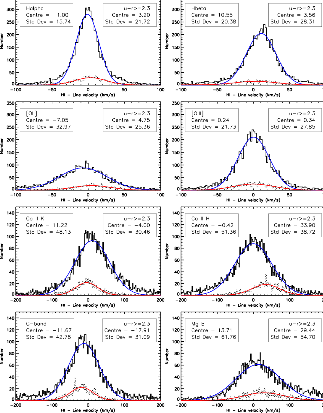
Figure 5: Comparison of velocities derived from individual spectral lines, compared to the ALFALFA H i velocity. The spectral feature is listed in the left-hand caption, along with the centre and width of the distributions. The emission lines (top four panels) all have significantly narrower distributions than the absorption lines (bottom four panels). The sub-samples in each panel show the reddest galaxies with $u-r\geq 2.3$, with the centres and widths of these distributions listed in the right-hand captions. The blue and red lines show the Gaussian curves fit to the full and red subsamples, respectively. Note the different x- and y-axis ranges for the emission and absorption panels.

Table 1: Summary of the distribution centres and standard deviations for each of the spectral features shown in Fig. 5.

			$u-r\geq 2.3$
Spectral	Centre	Std Dev	Centre	Std Dev
Feature	km s-1	km s-1	km s-1	km s-1
H$\alpha$	-1.00	15.74	3.20	21.72
H$\beta$	10.55	20.38	3.56	28.31
[O ii] 3727 Å	-7.05	32.97	4.75	25.36
[O iii] 5008 Å	0.24	21.73	0.34	27.85
Caii K 3935 Å	11.22	48.13	-4.00	30.46
Caii H 3970 Å	-0.42	51.36	33.90	38.72
G-band 4306 Å	-11.67	42.78	-17.91	31.09
Mg B 5177 Å	13.71	61.76	29.44	54.70

4 Simple Stacking Simulation

In order to quantify the effect the velocity difference distribution shown in Fig. 4 has on a putative stacked H i signal, we have constructed a simple spectral co-adding simulation. The simulation does not account for issues arising from the H i observations, such as RFI. We are purely interested in assessing the relative properties of the resulting stacked H i profiles when issues related to the accuracy of the optical spectrosocpy are incorporated.

The inputs of the simulation are the noise properties of the H i spectrum of a non-detection, a distribution of velocity offsets to represent the difference between the H i and optically determined redshifts, and a distribution of intrinsic H i widths. The noise is set to be Gaussian throughout, although there are indications that at some level the noise of real observations is not purely Gaussian (fig. 5 of Fabello et al. 2011 is a good illustration of this). The noise properties, in general, will be dependent on the instrument and observing conditions.

The H i profiles are modelled as two Gaussian curves each of fixed width, with separation either fixed at $W_{50}=150$ km s^-1, or drawn from the distribution of $W_{50}$ shown in Fig. 6, which closely approximates the H i $W_{50}$ distribution from the ALFALFA survey (see fig. 2b in Haynes et al. 2011). The two peaks of the H i profile vary in height with respect to each other, with about 30 per cent of the profiles having peaks differing in height by more than 20 per cent, which is broadly consistent the census of H i profile asymmetry from Richter & Sancisi (1994), who find 20 per cent of profiles are strongly asymmetric. A constant fills in the gap between the two profiles when it dips below half of the peak height. An example H i profile with the relevant features is shown in Fig. 7.

The velocity offset is either set to zero to simulate the case of identical optical and H i redshifts, a combination of 11 km s^-1 and 36 km s^-1 based on Fig. 4, or a series of increasing values representative of possible optical observations. The largest offset of 250 km s^-1 is loosely based on results from the redshift survey of the GOODS South field undertaken by Balestra et al. (2010). Using the VLT VIMOS instrument with the Low Resolution Blue grism (R$\sim$180), Balestra et al. (2010) find the redshift consistency for galaxies with more than one spectrum is measured to have a distribution of width 360 km s^-1, with the accuracy on a single redshift measurement of 360/$\sqrt{2}$=255 km s^-1. For the Medium Resolution orange grism (R$\sim$580), the redshift consistency distribution has width 168 km s^-1, and the accuracy for a single measurement of 120 km s^-1. These determinations of redshift accuracy indicate the difficulty of obtaining accurate measures of high redshift galaxies, even with an 8-m class telescope.

We use two separate methods for setting the peak of the undetected H i profiles with respect to the noise. In the first case, one peak of the H i profiles is given in terms of a fraction of the sigma of the noise, while the other peak can be larger or smaller. Here, we set the peak to be 1$\sigma$, to give a peak S/N $=1$. For convenience, we refer to these profiles as the constant peak profiles, and an example of this profile type is shown in Fig. 7.

The second case sets a reference profile of width $W_{50}=150$ km s^-1 and peak height of 1$\sigma$. The integrated area under this curve is computed and used as the reference area. We scale all the other curves of varying widths such that the area under their curves is equal to the reference area. Physically, as the area under the profile curve is a measure of the H i mass of a galaxy, this case describes an ensemble of galaxies of equal H i masses within a redshift shell. Narrower profiles end up with peak S/N $>1$ and wider profiles have S/N $<1$, but all have the same integrated signal. We refer to these profiles as the constant area profiles.

The constant peak and constant area profiles span a range of input H i mass distributions, from combining galaxies of different masses (constant peak profiles) to combining galaxies all of the same mass (constant area profiles), while maintaining the observationally determined distribution of H i profile widths. The results allow us to begin to understand the relative importance of the input H i mass distribution into the stacked signal by comparing the resulting profiles.

Figure 6: The input H i $W_{50}$ width distribution for the stacking simulations, which is an approximation to the distribution shown in fig. 2b of Haynes et al. (2011).

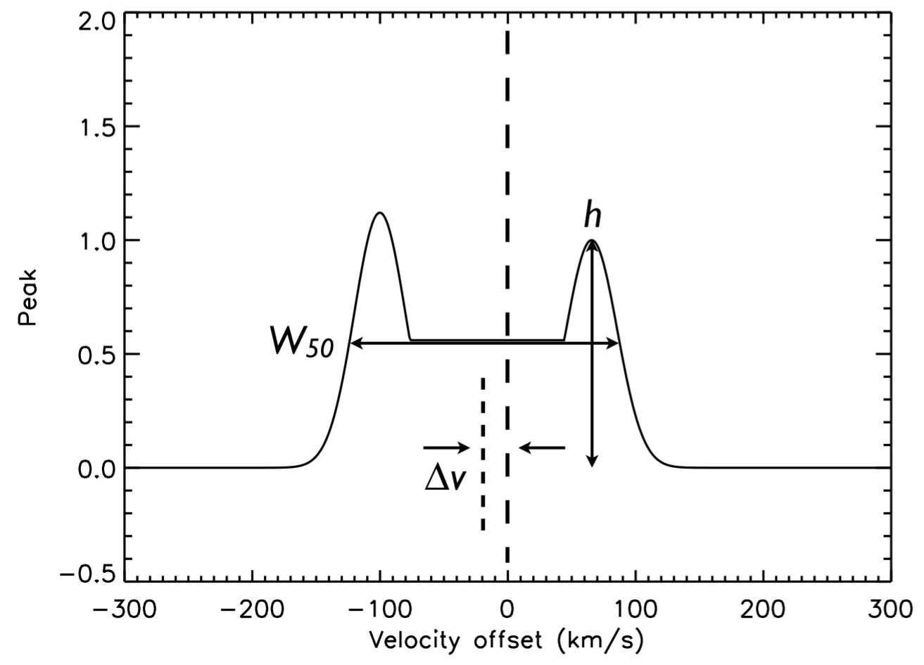
Figure 7: The variable parameters for the simulated H i profiles for the stacking simulations. The height of one peak, h, is set to unity, with the height of the other peak varying with respect to this.

A number of simulations are presented here to facilitate comparison. The parameters for each are listed in Table 2. Simulations with $W_{50}$ listed as Fixed are unphysical as the profiles are all of identical widths, but serve as a useful reference point and show the effect of the velocity offset only. Similarly for simulations 2 and 3, the effect of the H i distribution is isolated, as the velocity offset is set to zero. Simulations 5 and 6 represent the scenario that most closely matches the data we have from the ALFALFA H i profiles and the corresponding SDSS spectra. Simulations 20 and 21 show the effect of much poorer quality optical spectra.

For each combination of parameters, we simulate 1000 spectra, with the parameters drawn from the velocity offset and $W_{50}$ distributions. For the velocity offsets based on Fig. 4, parametrized with two Gaussians, one in three offsets is chosen from the wide profile, to approximate the relative contributions of the wide and narrow components. The 1000 constructed spectra are stacked in no particular order, using a simple averaging for each channel, following:

$$S=\frac{\sum_{i=1}^{1000}S_{i}w_{i}}{\sum_{i=1}^{1000}w_{i}}$$ (1)

where $S_{i}$ are the individual spectra, $w_{i}$ are weights for each spectrum as the inverse of the square of the spectrum RMS noise, and $S$ is the stacked spectrum. For the simulations, the weights are ignored as the noise of each spectrum is the same. The progress of the resulting stacked spectrum is followed with each additional spectrum. This process is repeated 50 times for each set of parameters to ensure the distributions are fully sampled and the results are averaged.

Table 2: Variables incorporated various runs of the simulations. Profile type = P indicates constant peak profiles, and Profile type = A indicates constant area profiles.

Number	Velocity Offset	$W_{50}$	Profile Type
	Dist’n Width (km s-1)	Dist’n
1	0	Fixed	P
2	0	Variable	P
3	0	Variable	A
4	11/36	Fixed	P
5	11/36	Variable	P
6	11/36	Variable	A
7	60	Fixed	P
8	60	Variable	P
9	60	Variable	A
10	100	Fixed	P
11	100	Variable	P
12	100	Variable	A
13	150	Fixed	P
14	150	Variable	P
15	150	Variable	A
16	200	Fixed	P
17	200	Variable	P
18	200	Variable	A
19	250	Fixed	P
20	250	Variable	P
21	250	Variable	A

5 Simulated Stacked Spectra

Here we describe the outcome of the simulations described in Section 4, including the changes in profile shape, how the stacked profile flux compares to the fluxes of the input galaxies, and what we can learn about stacking in the context of future survey design.

5.1 The Stacked Profiles

The stacked profiles from 1000 spectra corresponding to simulations 1, 4, 7, 10, 13, 16 and 19 (profiles of fixed width) are shown in Fig. 8, divided by the number of input spectra, and averaged over the 50 iterations. The double-peaked profile shape is only visible while the velocity errors are small. While these profiles are unrealistic as they are drawn from a set of identical H i profiles representing identical galaxies, they isolate the effect of the redshift errors from the distribution of input profile widths. Once the velocity errors are larger than 11 km s^-1, the width of the profile is no longer well measured by $W_{50}$, so we fit a Gaussian to the curve and measure the standard deviation. Table 3 lists the standard deviations for each of the profiles shown in Figs.  8 through 10. The noise measured in channels 0–300 and 1700–2000, away from the signal for each stacked spectrum after combining $n$ spectra, retains Gaussian behaviour.

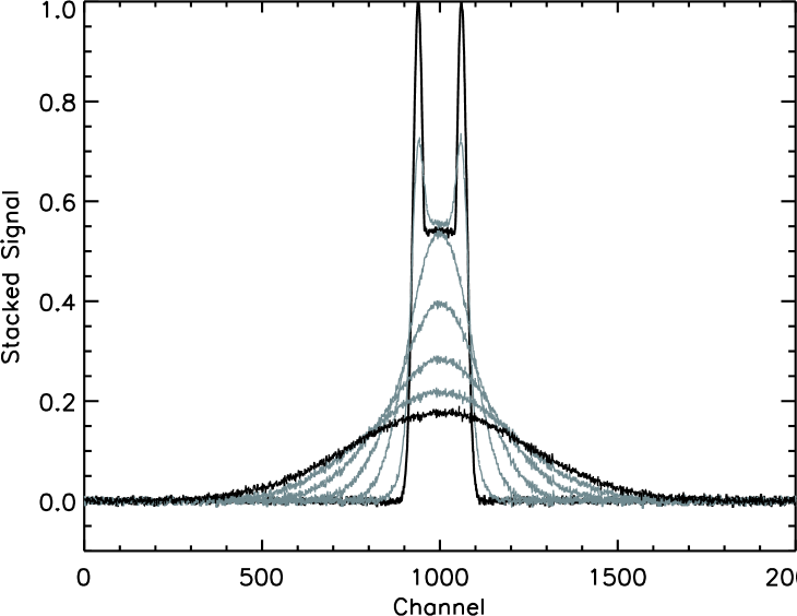
Figure 8: Comparison of the stacked profiles for 1000 constant peak profiles of fixed width ($W_{50}=150$ km s^-1) and velocity offset distribution widths $\Delta v$=0, 11/36, 60, 100, 150, 200, 250 km s^-1 (top to bottom), averaged over 50 iterations. The x-axis is incremented by ones, so each point corresponds to a ‘channel’ of width 1 km s^-1. Each profile has been divided by 1000, the number of input spectra.

The stacked profiles from 1000 spectra corresponding to the constant peak profiles with varying widths (simulations 2, 5, 8, 11, 14, 17 and 20) are shown in Fig. 9. Note that the input double-peaked profile is washed out in all of the stacked profiles by the distribution of input profile widths, and the width of the profiles with large $\Delta v$ become wider than the median input width of $W_{50}=150$ km s^-1.

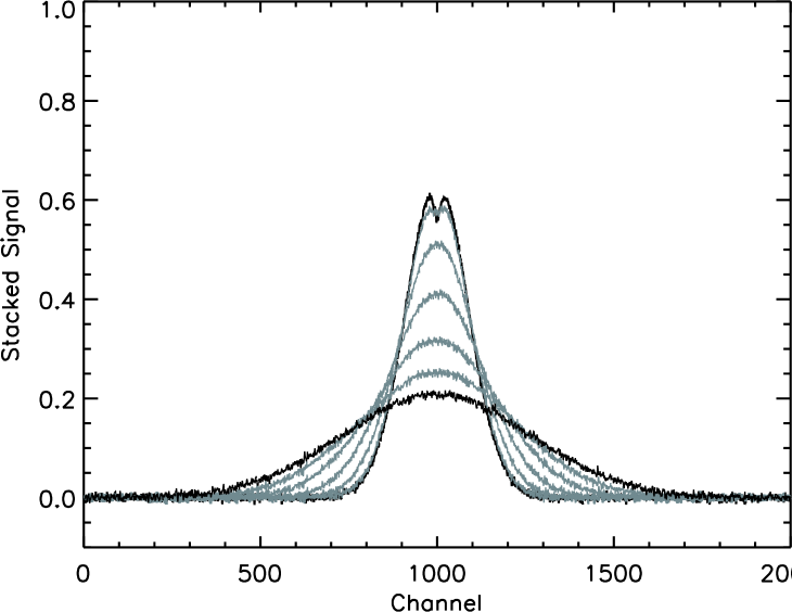
Figure 9: Comparison of the stacked profiles for 1000 constant peak profiles and velocity offsets $\Delta v$=0, 11/36, 60, 100, 150, 200, 250 km s^-1 (top to bottom), averaged over 50 iterations.

Fig. 10 shows the stacked profiles corresponding to the constant area profiles (simulations 3, 6, 9, 12, 15, 18 and 21). The resulting H i profiles are slightly narrower than for the constant peak profiles, due to the relatively strong contribution from narrow input profiles and the weaker contribution from wide profiles, but otherwise the profiles in Figs. 9 and 10 are very similar. This indicates that the relative width of the stacked profile is more sensitive to the input profile width distribution rather than the input H i mass distribution, particularly when the velocity offset distribution width is large.

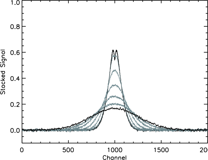
Figure 10: Comparison of the stacked profiles for 1000 constant area profiles and velocity offsets $\Delta v$=0, 11/36, 60, 100, 150, 200, 250 km s^-1(top to bottom), averaged over 50 iterations.

Table 3: Standard deviations of the profiles shown in Figs.  8 through 10. All values are in km s^-1.

Velocity	Fixed	Constant	Constant
Offset	Width	Peak	Area
0	63	92	73
11/36	68	95	76
60	86	111	97
100	117	138	127
150	161	177	168
200	209	222	216
250	255	269	258

5.2 Derived Fluxes of Stacked Profiles

One of the goals of H i stacking is to derive an average mass for the contributing galaxies. We therefore investigate how the measured mass of the stacked profiles compares to the masses of the input galaxies. As the relationship between flux and mass has a straightforward distance dependence, we compute only fluxes for our input and stacked profiles, with the understanding that the fluxes can easily be converted into masses. With real data, redshifts to individual contributing objects will be known from the optical spectroscopy.

The flux of each of the 1000 individual contributing profiles is measured before adding noise by integrating over the 2000 channels. Both the average and median of these input fluxes are calculated for comparison with the flux in the stacked profile.

To compute the flux of the stacked profiles, we integrate under each of the curves shown in Figs. 8 through 10. For the narrow profiles with small velocity offsets, the edges of the profiles are obvious, thus the limits of integration are well determined. However, for the wider profiles, the limits of the profile are not as well defined. Therefore, for each profile that is well fit by a Gaussian, we find the centre and sigma of the fit, and integrate over $\pm$3$\sigma$. For narrow, non-Gaussian shaped profiles, or profiles with low S/N, we simply integrate over the entire 2000 channels, as regions without signal will average to zero since the noise is Gaussian-distributed about zero. This may not be the case for stacking real data, as low-level ripples from standing waves in single dish data, such as that found by Fabello et al. (2011), or low-level RFI, sidelobes from undetected sources in the field, and other calibration issues in interferometric data will cause the stacked noise to be non-Gaussian.

We find that we are able to recover the average flux of the input profiles from the stacked profile, with no dependence on the velocity offsets, and thus the stacked profile width. For the constant peak profiles with variable widths, the flux in the stacked profile is larger than the average flux of the input profiles by 1–2 per cent. It is larger than the median flux of the input profiles by 6–7 per cent, indicating that the rarer, larger input profiles significantly contribute to the stacked profile. The profiles with constant widths show similar behaviour as the constant peak profiles. For the constant area profiles, the average and median input profile fluxes are identical, and differ from the stacked profile flux by less than one per cent. Therefore, in these ideal cases, the flux contained within the stacked profile is a good representation of the average flux of the input profiles.

5.3 Applications to Future Surveys

The dependence of the stacked profile width on the quality of optical redshifts is useful for justifying requirements for spectroscopic ancillary data for upcoming H i deep field surveys. We have demonstrated that the width of a stacked H i profile is dependent on the $W_{50}$ distribution of input H i profiles for small differences between the optical and H i velocities. When the velocity errors are comparable to or larger than the median $W_{50}$ width of the input profiles, they dominate the stacked profile width.

By combining the results of the stacking simulations with a relationship between the measured flux of a stacked signal and the integrated signal to noise, we can predict the average H i mass detectable from a stacked profile at a particular redshift, given a specified integrated S/N and the parameters of the survey and instrumentation.

We start with the equation for integrated S/N from Haynes et al. (2011):

$$\frac{S}{N}=\frac{1000\,S_{21}}{W_{50}}\frac{\omega_{smo}^{1/2}}{\sigma}$$ (2)

where $1000\,S_{21}$ is the integrated flux in mJy km s^-1, $W_{50}$ is the full width at half max of the H i profile, and $\sigma$ is the noise in mJy of the signal-free portion of the spectrum. $\omega_{smo}$ is a ‘smoothing width’, which for the ALFALFA survey is defined as $\omega_{smo}=W_{50}/(2\times 10)$ for profiles less than 400 km s^-1 wide, and 10 is the spectral resolution in km s^-1 for the final ALFALFA cubes. Hereinafter, we express the channel width as $\Delta w$ to generalize the smoothing width to any survey.

Equation 2 is appropriate for individual H i profiles with relatively steep sides, where $W_{50}$ is a good measure of the width of the profile and encompasses most of the flux. However, as seen in Figs. 8, 9 and 10, the sides of stacked signals are not steep, and $W_{50}$ is no longer a good approximation to the full width over which flux is measured. In order to include the majority of the flux in the stacked profiles, instead of $W_{50}$, we use $W_{full}$, which we define as $\pm 3$ times the standard deviation of a Gaussian function fit to the stacked H i profile. This is also the range over which we integrate the stacked profiles from the simulations to compute the total flux. Equation 2 is then rewritten as:

$$\frac{S}{N}=\frac{1000\,S_{21}}{\sigma\,W_{full}}\left(\frac{W_{full}}{2\,\Delta w}\right)^{1/2}.$$ (3)

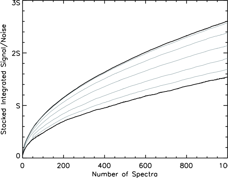
Figure 11: Comparison of the integrated S/N of the profiles shown in Fig. 9 for velocity offsets $\Delta v$=0, 11/36, 60, 100, 150, 200, 250 km s^-1 (top to bottom). The integrated S/N value at 1000 spectra corresponds to the profiles shown in Fig. 9. The scale on the y-axis is arbitrary, with units of S representing integrated S/N.

A measure of the integrated S/N of the stacked H i constant peak profiles and how it grows with adding more stacked spectra is shown in Fig. 11. The integrated S/N grows faster for narrower profiles. The $S/N$ for each of the three profile types show similar behaviour. For large velocity offsets and small numbers of input spectra, the stacked profile is not well-defined, so we simply integrate the stacked signal between 300–1700 channels. The transition between integrating over a set range and integrating over $W_{full}$ is visible for small numbers of input spectra as a discontinuity in the curve. The noise does not contribute significantly to the total flux.

For H i masses at any redshift, the well-known H i mass equation is:

$$\frac{M_{HI}}{M_{\odot}}=\frac{2.36\times 10^{5}\,D^{2}}{1+z}\int S_{v}\,dv\\$$ (4)

where $M_{HI}$ is the total H i mass in solar masses, $D$ is the luminosity distance to the object in Mpc, and the integral is the total flux in Jy km s^-1, equivalent to $S_{21}$ in equations 2 and 3. The $1+z$ factor accounts for the difference between the observed and rest-frame width of the measured profile. Rewriting equation 4 in terms of equation 3:

$$\frac{M_{HI}}{M_{\odot}} = \frac{2.36\times 10^{5}\,D^{2}}{1+z}S_{21}$$ (5)

$$= \frac{2.36\times 10^{5}\,D^{2}}{1+z}\,\frac{(2\,\Delta w\,W_{full})^{1/2}\,\sigma}{1000}\,\frac{S}{N}.$$ (6)

This is the total H i mass in solar masses for a given profile. Assuming that the noise is fairly flat over the frequency range surveyed, which is not unreasonable (Fernández et al. 2013), then the noise of the stacked spectrum is related to the noise of a single spectrum (the inherent noise of a survey, $\sigma_{1}$) by $\sigma=\sigma_{1}n_{spec}^{1/2}$. By dividing both sides of the mass equation by the number of spectra stacked, we can express the average H i mass per contributing object from a stacked signal as:

$$\left<\frac{M_{HI}}{M_{\odot}}\right>=2.36\times 10^{5}\,\left<\frac{D^{2}}{1+z}\right>\frac{(2\,\Delta w\,W_{full})^{1/2}}{1000}\,\frac{\sigma_{1}}{n^{1/2}_{spec}}\,\frac{S}{N}.$$ (7)

The advantage of expressing the H i mass in this way is that all but one of the variables are either defined by the observation parameters ($\Delta w$, $\sigma_{1}$) or they can be estimated for a specific scenario, for example the number of spectra available to stack in a given redshift shell ($D$ and $1+z$, $S/N$, $n_{spec}$). The remaining variable, $W_{full}$, can be estimated from our stacking simulations. From Figs. 8 through 10, $W_{full}$ depends on the distribution of optical–H i velocity differences for the galaxies input into the stacked profile, parametrized by the velocity offset in the stacking simulations.

As seen in Fig. 11, the number of spectra required to reach a given integrated S/N increases with increasing stacked profile width. Fig. 12 shows the relative number of constant peak profile spectra required to reach $S/N=$ 0.6S, 0.8S and S, which is equivalent to making three horizontal cuts in Fig. 11. The behaviour is similar for the constant width and constant area profiles. Approximately twice as many spectra are required for the largest velocity offsets compared with velocity offsets $<100$ km s^-1. For large $S/N$, an arbitrarily large number of spectra would be required for the widest profiles. Conversely, given a finite number of spectra available for stacking, the integrated S/N that can be achieved is reduced for larger velocity offsets.

Figure 12: Comparison of the relative number of spectra required to achieve an integrated S/N=0.6S, 0.8S and S for velocity offsets $\Delta v$=0, 11/36, 60, 100, 150, 200, 250 km s^-1 and the constant peak profiles.

Fig. 13 shows how the relative H i mass sensitivity changes with increasing stacked H i profile width for the constant peak profiles. This is effectively taking a vertical cut through Fig. 11. For a given redshift, the H i mass sensitivity achieved with a given number of spectra improves by a factor of $\sim$1.7 as the width of the H i profile decreases.

Figure 13: Comparison of the H i mass sensitivity for 1000 spectra and integrated S/N=S, for velocity offsets $\Delta v$=0, 11/36, 60, 100, 150, 200, 250 km s^-1.

6 Discussion

The results of the ALFALFA–SDSS redshift comparison and the simulations enable us to make some general recommendations regarding observation strategies in preparation for surveys that will employ H i stacking. As the H i will be undetected, any useful quantities must be derived from the optical data. We also discuss how the results presented here will apply to future telescopes and surveys at high redshift.

6.1 General Recommendations

The success of H i stacking depends heavily on the quality of the optical spectroscopy. The spectral resolution of the SDSS spectra, at about R=1800–2200, is sufficient to resolve spectral features such as the H$\alpha$, [N ii] and H$\beta$, [O iii] emission line groups. From the ALFALFA–SDSS comparison, these spectra, with accurate wavelength calibration, give redshifts that match the H i redshifts to within tens of km s^-1. Measuring a single spectral feature does not give as accurate redshifts as using a number of features, but from the simulations, we see that as long as the difference between the optical and H i redshifts are less than the median width of the H i profiles, the stacked profile shape is largely unaffected by the redshift uncertainties. This is in qualitative agreement with work by Khandai et al. (2011), who find that redshift errors of $\Delta z<35$ km s^-1 dilute their simulated stacked profile peak by less than 3 per cent.

Photometric redshifts are one technique used to circumvent telescope-intensive spectroscopy, and have successfully been applied to extract a number of cosmological results (see, for example, the COMBO-17 project, Wolf et al. 2004). However, even discarding the galaxies assigned redshifts that greatly differ from the real value, referred to as catastrophic outliers, the redshift accuracy achieved is of the order $\Delta z/(1+z)>0.01$, corresponding to velocity uncertainties of several thousands of km s^-1. From Figs. 9 and 10, the resulting profile will be unreasonably wide, and the integrated SNR will hardly increase with additional stacked objects, using the simple stacking procedure followed here. However, photometric redshifts will certainly be useful for pre-selection of galaxy targets in redshift shells, allowing highly efficient follow-up observations with moderate resolution spectroscopy.

Galaxies with red optical colours also seem to produce less accurate redshifts. It may be tempting to target only blue, star-forming galaxies and ignore the red, absorption line galaxies in spectroscopic campaigns, but there is evidence that spheroids contain a non-negligible amount of cold gas (see, for example, Grossi et al. 2009, Serra et al. 2012), and should thus be included in an H i census. However, if the goal is to construct the cleanest stacked spectrum possible, excluding red galaxies is a possibility for particular cases.

As the current and future surveys will encompass large volumes, acquiring spectroscopy of every galaxy in the survey volume is unrealistic. It also may be large effort for low gain, as can be seen in Fig. 11. For small numbers of spectra, the integrated S/N increases rapidly, but after a few hundred spectra, the S/N increases much slower with additional spectra. This is particularly true for lower quality (large velocity error) spectra. Therefore, consideration of the number of galaxies available for stacking, and the quality of the optical spectra to be collected, is necessary for planning the ancillary data collection. Equation 7 will be useful for this planning.

6.2 Future Telescopes and Surveys at High Redshift

The results presented in this paper are based on galaxies in the local Universe, observed with a single-dish radio telescope. Ongoing and upcoming surveys are almost exclusively being undertaken with interferometers, such as the CHILES project with the JVLA, LADUMA with MeerKAT, and DINGO with ASKAP. These facilities all have significantly better spatial resolution than Arecibo. This will be useful for separating close pairs of galaxies which would be unresolved in single dish data.

The expanded frequency range of upcoming facilities, particularly of MeerKAT, will enable H i studies to progress to $z\sim 1.4$. The galaxy population has undergone significant evolution from $z=1$ to the present, so it is interesting to consider how the results from this $z\sim 0$ study may apply at high redshifts. The fraction of interacting galaxies is known to increase with redshift (Conselice, Yang, & Bluck 2009), which will contribute to the outlier population in the optical–H i redshift differences, resulting in a broader stacked H i profile. The higher star-formation rate at $z\sim 1$ produces greater galactic outflows, of order $\sim$300 km s^-1, which will also affect the measured optical redshifts (see, for example, Weiner et al. 2009 and Kornei et al. 2012).

We found that when the optical–H i redshift differences are of the same order as the median H i width, the stacked profile begins to significantly broaden. From the ALFALFA survey, the median width is $W_{50}\sim 150$ km s^-1 at $z=0$, but this value is unknown at $z>0.5$. Simulations from Obreschkow et al. (2009) suggest that the size of the H i disk of a Milky Way type galaxy will decrease by a factor of two between $z=0-1.5$, with a similar decrease in H i mass. If the H i disks become significantly smaller, the median $W_{50}$ will also decrease, and the optical redshifts will need to be of correspondingly better quality.

H i-rich satellite galaxies have not been incorporated in the current study, and will most likely be undetected in both the optical and radio data. They may, however, appear in a stacked profile, both in the wings and the central region of the profile (Khandai et al., 2011). Observationally, at $z=0$ satellites account for only one per cent of the total H i of the Milky Way, and including the satellites predicted by $\Lambda$CDM simulations, this increases to $\sim$10 per cent (Grcevich & Putman, 2009), and may become increasingly important at higher redshift where more galaxy assembly is taking place.

7 Conclusions

We have conducted an investigation into the relationship between galaxy redshifts derived from optical spectroscopy and radio H i observations using galaxies from the ALFALFA survey matched to the SDSS. We find that the redshifts match well, with negligible offset. The width of the distribution is well approximated with two Gaussians, the narrow core having a width of 11 km s^-1 and the broad wings having 36 km s^-1. The width of the distribution is narrower if many optical spectral features are used to measure the redshift instead of only one feature. The $u-r$ colour was the only optical property of the galaxies found that correlated with redshift offset, with red galaxies preferentially lying in the wings of the redshift difference distribution. Disturbed or interacting systems, as well as galaxies with asymmetric H i profiles also preferentially have large redshift offsets.

We have constructed simple simulations to investigate the effect redshift uncertainties have on a stacked H i profile. The simulations span a range of input mass functions, with the resulting stacked profiles being similar in each case. In addition to using the velocity differences derived from the ALFALFA–SDSS galaxies, we also input a number of increasing velocity differences in order to determine at which point the redshift errors dominate the properties of the stacked profile. We find that for redshift errors less than the median width of the input profiles, the distribution of profile widths is the dominant effect which broadens the stacked profile. For larger redshift errors, the input distribution of profile widths becomes insignificant and the redshift errors broaden the stacked profile.

We have computed the flux for each of the contributing profiles as well as the flux of the resulting stacked profile, and find that the recovered flux from the stack matches the average input flux to within a few per cent. We have also provided an equation relating the H i mass sensitivity of a stacked profile in terms of telescope and survey parameters, which will be useful for estimating the number of spectra required to reach a given average H i mass. This should, however, be treated as an optimistic case, as the noise in these simulations is Gaussian and may not be representative of the noise that will be present in real, interferometric radio data, which will be contaminated by RFI and bright continuum sources.

References

- Abazajian et al. (2009) Abazajian K. N., et al., 2009, ApJS, 182, 543
- Adelman-McCarthy et al. (2008) Adelman-McCarthy J. K., et al., 2008, ApJS, 175, 297
- Baldry et al. (2004) Baldry I. K., Glazebrook K., Brinkmann J., Ivezić Ž., Lupton R. H., Nichol R. C., Szalay A. S., 2004, ApJ, 600, 681
- Balestra et al. (2010) Balestra I., et al., 2010, A&A, 512, A12
- Barnes et al. (2001) Barnes D. G., et al., 2001, MNRAS, 322, 486
- Brinchmann et al. (2004) Brinchmann J., Charlot S., White S. D. M., Tremonti C., Kauffmann G., Heckman T., Brinkmann J., 2004, MNRAS, 351, 1151
- Catinella et al. (2008) Catinella B., Haynes M. P., Giovanelli R., Gardner J. P., Connolly A. J., 2008, ApJ, 685, L13
- Chang et al. (2010) Chang T.-C., Pen U.-L., Bandura K., Peterson J. B., 2010, Natur, 466, 463
- Chengalur, Braun, & Wieringa (2001) Chengalur J. N., Braun R., Wieringa M., 2001, A&A, 372, 768
- Chung et al. (2009) Chung A., van Gorkom J. H., Kenney J. D. P., Crowl H., Vollmer B., 2009, AJ, 138, 1741
- Conselice, Yang, & Bluck (2009) Conselice C. J., Yang C., Bluck A. F. L., 2009, MNRAS, 394, 1956
- Delhaize et al. (2013) Delhaize J., Meyer M., Staveley-Smith L., Boyle B., 2013, arXiv, arXiv:1305.1968
- Dunne et al. (2009) Dunne L., et al., 2009, MNRAS, 394, 3
- Fabello et al. (2011) Fabello S., Catinella B., Giovanelli R., Kauffmann G., Haynes M. P., Heckman T. M., Schiminovich D., 2011, MNRAS, 411, 993
- Fernández et al. (2013) Fernández X., et al., 2013, arXiv, arXiv:1303.2659
- Garcia-Appadoo et al. (2009) Garcia-Appadoo D. A., West A. A., Dalcanton J. J., Cortese L., Disney M. J., 2009, MNRAS, 394, 340
- Giovanelli et al. (2005) Giovanelli R., et al., 2005, AJ, 130, 2598
- Giovanelli et al. (2005) Giovanelli R., et al., 2005, AJ, 130, 2613
- Giovanelli et al. (2007) Giovanelli R., et al., 2007, AJ, 133, 2569
- Grcevich & Putman (2009) Grcevich J., Putman M. E., 2009, ApJ, 696, 385
- Grossi et al. (2009) Grossi M., et al., 2009, A&A, 498, 407
- Haynes, Giovanelli, & Kent (2007) Haynes M. P., Giovanelli R., Kent B. R., 2007, ApJ, 665, L19
- Haynes et al. (2011) Haynes M. P., et al., 2011, AJ, 142, 170
- Holwerda et al. (2012) Holwerda B. W., Blyth S.-L., Baker A. J., Baker, 2012, IAUS, 284, 496
- Hopkins & Beacom (2006) Hopkins A. M., Beacom J. F., 2006, ApJ, 651, 142
- Jaffé et al. (2013) Jaffé Y. L., Poggianti B. M., Verheijen M. A. W., Deshev B. Z., van Gorkom J. H., 2013, arXiv, arXiv:1302.1876
- Johnston et al. (2008) Johnston S., et al., 2008, ExA, 22, 151
- Jonas (2009) Jonas J. L., 2009, IEEEP, 97, 1522
- Karim et al. (2011) Karim A., et al., 2011, ApJ, 730, 61
- Khandai et al. (2011) Khandai N., Sethi S. K., Di Matteo T., Croft R. A. C., Springel V., Jana A., Gardner J. P., 2011, MNRAS, 415, 2580
- Kornei et al. (2012) Kornei K. A., Shapley A. E., Martin C. L., Coil A. L., Lotz J. M., Schiminovich D., Bundy K., Noeske K. G., 2012, ApJ, 758, 135
- Lagos et al. (2011) Lagos C. D. P., Baugh C. M., Lacey C. G., Benson A. J., Kim H.-S., Power C., 2011, MNRAS, 418, 1649
- Lah et al. (2007) Lah P., et al., 2007, MNRAS, 376, 1357
- Lah et al. (2009) Lah P., et al., 2009, MNRAS, 399, 1447
- Madau, Pozzetti, & Dickinson (1998) Madau P., Pozzetti L., Dickinson M., 1998, ApJ, 498, 106
- Martin et al. (2010) Martin A. M., Papastergis E., Giovanelli R., Haynes M. P., Springob C. M., Stierwalt S., 2010, ApJ, 723, 1359
- Meyer et al. (2004) Meyer M. J., et al., 2004, MNRAS, 350, 1195
- Obreschkow et al. (2009) Obreschkow D., Croton D., De Lucia G., Khochfar S., Rawlings S., 2009, ApJ, 698, 1467
- de Ravel et al. (2009) de Ravel L., et al., 2009, A&A, 498, 379
- Richter & Sancisi (1994) Richter O.-G., Sancisi R., 1994, A&A, 290, L9
- Serra et al. (2012) Serra P., et al., 2012, MNRAS, 422, 1835
- Toribio et al. (2011) Toribio M. C., Solanes J. M., Giovanelli R., Haynes M. P., Masters K. L., 2011, ApJ, 732, 92
- Tremonti et al. (2004) Tremonti C. A., et al., 2004, ApJ, 613, 898
- Verheijen et al. (2008) Verheijen M. A. W., Oosterloo T. A., van Cappellen W. A., Bakker L., Ivashina M. V., van der Hulst J. M., 2008, AIPC, 1035, 265
- Weiner et al. (2009) Weiner B. J., et al., 2009, ApJ, 692, 187
- Wolf et al. (2004) Wolf C., et al., 2004, A&A, 421, 913
- Wong et al. (2006) Wong O. I., et al., 2006, MNRAS, 371, 1855
- York et al. (2000) York D. G., et al., 2000, AJ, 120, 1579
- Zwaan et al. (2005) Zwaan M. A., Meyer M. J., Staveley-Smith L., Webster R. L., 2005, MNRAS, 359, L30