A versatile simulator for specular reflectivity study of multi-layer thin films

Abstract

A versatile X-ray/neutron reflectivity (specular) simulator using LabVIEW (National Instruments Corp.) for structural study of a multi-layer thin film having any combination, including the repetitions, of nano-scale layers of different materials is presented here (available to download from the link provided at the end). Inclusion of absorption of individual layers, inter-layer roughnesses, background counts, beam width, instrumental resolution and footprint effect due to finite size of the sample makes the simulated reflectivity close to practical one. The effect of multiple reflection is compared with simulated curves following the exact dynamical theory and approximated kinematical theory. The applicability of further approximation (Born theory) that the incident angle does not change significantly from one layer to another due to refraction is also considered. Brief discussion about reflection from liquid surface/interface and reflectivity study using polarized neutron are also included as a part of the review. Auto-correlation function in connection with the data inversion technique is discussed with possible artifacts for phase-loss problem. An experimental specular reflectivity data of multi-layer erbium stearate Langmuir-Blodgett (LB) film is considered to estimate the parameters by simulating the reflectivity curve.

I Introduction

The reflectivity study is a very powerful scattering technique parratt ; russell ; gibaud ; tolan ; nielsen ; physrep performed at grazing angle of incidence to study the structure of surface and interface of layered materials, thin films when the length scale of interest is in nm regime. Utilizing the intrinsic magnetic dipole moment of neutron, the neutron reflectivity study provides magnetic structure in addition with the structural information. In reflectivity analysis, the electron density (ED)/scattering length density (SLD) (in case of X-ray/neutron) of different layers along the depth is estimated by model-fitting the experimental data. Text-based language like FORTRAN is commonly used to write a simulation and data analysis code. However, recently a graphical language LabVIEW ((Laboratory Virtual Instrument Engineering Workbench, from National Instruments Corp.) has emerged as a powerful programming tool for instrument control, data acquisition and analysis. It offers an ingenious graphical interface and code flexibility thereby significantly reducing the programming time. The user-friendly and interactive platform of LabVIEW is utilized, here, to simulate a versatile angle-resolved reflectivity at glancing angles. There is only a recent report praman of LabVIEW-based reflectivity simulator for energy-resolved reflectivity study where the effects of absorption and interfacial roughnesses are not included. The center for X-ray optics (CXRO) provides a similar online simulator, however, the LabVIEW-based simulator has complete freedom to customize the programme according to user’s choice.

Let us start with brief review on theoretical formalisms of specular reflectivity with LabVIEW simulated curves. Scattering geometry for specular scan, polarized neutron reflectivity and reflectivity from liquid surface are discussed in the next section. Data inversion technique and the phase problem are discussed then considering the Auto-correlation function (ACF). Finally, the LabVIEW-based reflectivity simulator is discussed in detail.

II Study of grazing-incidence reflectivity with LabVIEW simulated curves

The basic quantity that is measured in a scattering experiment nielsen ; sivia is the fraction of incident flux (intensity of X-ray/number of neutrons) that emerges in various directions is known as the differential cross-section. Normalizing this quantity by the incident intensity and density of scatterer, one obtains the scattering rate, $R$ which is termed as reflectivity (merely, differed by some constant in different convention and dimensionality) in nano-scale study of materials at grazing angle. For elastic scattering, $R$ depends only on the momentum transfer, $\overrightarrow{q}$ which can be varied by varying the energy (energy-resolved reflectivity) of the incident beam i.e. with a white beam at a fixed grazing incident angle or by varying the incidence angle (angle-resolved reflectivity) using monochromatic beam. The angle-resolved reflectivity which is common in practise for its better resolution is discussed here. In following discussion We consider, mainly, X-ray reflectivity however the formalism holds exactly the same way for neutron reflectivity considering SLD instead of ED.

The Born Formalism: In quantum mechanical treatment, the incident beam, represented by a plane wave emerges out as spherical wave when interacted with the scattering potential. Incident plane is related to the emerging spherical wave through the integral scattering equation. In first Born approximation of the integral scattering equation, the scattering amplitude depends on the Fourier transforation (FT) of the scattering potential. When the scatterer is composed of homogeneous layers parallel to the x-y plane, the scattering amplitude, in the first-order approximation, depends only on the FT of the gradient of ED along the z-axis, implying the expression for reflectivity parratt ; russell ; gibaud ; tolan ; nielsen ; physrep ; sivia as:

$$R(q_{z})=\frac{(4\pi r_{e})^{2}}{q^{4}_{z}}\left|\int_{-\infty}^{+\infty}\frac{d\rho(z)}{dz}e^{iq_{z}z}dz\right|^{2}$$ (1)

where $\rho(z)$ is the ED at depth z (from top of the sample) averaged over the x-y plane, $r_{e}=e^{2}/{m_{e}c^{2}}=2.818\times 10^{-5}$ Å is classical radius of electron, or the Thomson scattering length.

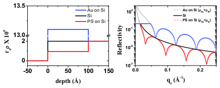
Figure 1: The ED profile, $\rho(z)$ and the Born approximated reflectivity curves for bare Si-substrate (black curve), a 100 Å thick single layer of Poly-sterene (PS) (red curve) and Au (blue curve) ($\rho_{Au}>\rho_{Si}>\rho_{PS}$) on Si-substrate. For small values of $q_{z}$, the failure of the model is obvious as $R$ becomes more than unity (grey curves). The oscilations (Kiessig fringes) with $\Delta q_{z}=0.0628$ Å^-1 exactly corresponds to the layer-thickness, $d=2\pi/{\Delta q_{z}=}$100 Å. Interesting to note that, the overall level of the reflectivity curve is higher or lower depending upon whether the ED of a layer is greater or less than that of the substrate.

In the simplest possible situation where scattering from a bare substrate is considered, the ED is a step function:

$$\rho(z)=\begin{cases}\rho_{s}&\text{for }z<0,\\ 0&\text{for }z>0.\end{cases}$$

Obviously,

$$\frac{d\rho}{dz}=-\rho_{s}\delta(z)$$

where $\delta(z)$ is the Dirac’s Delta function. Using the integral property of Delta fn.

$$\int_{-\infty}^{+\infty}\delta(z-0)e^{iq_{z}z}dz=e^{0}=1$$

Eqn. (1) implies,

$$R(q_{z})=\frac{(4\pi r_{e}\rho_{s})^{2}}{q^{4}_{z}}\equiv R_{F}(q_{z})$$ (2)

$R_{F}(q_{z})$ is known as the Fresnel reflectivity which does not hold at small angle as eqn. (2) violates the physical constraint that $R\leq 1$ as $q_{z}\rightarrow 0$. This limitation is a consequence of neglecting the higher order terms of the scattering integral equation in first-order Born approximation. Using eqn. (2), one can rewrite eqn. (1) as

$$R(q_{z})=R_{F}(q_{z})\left|\frac{1}{\rho_{s}}\int_{-\infty}^{+\infty}\frac{d\rho(z)}{dz}e^{iq_{z}z}dz\right|^{2}$$ (3)

When there is a uniform layer of thickness, $d$ on a substrate (refer to Fig. 1), the ED are given by:

$$\rho(z)=\begin{cases}\rho_{s}&\text{for }z<-d,\\ \rho_{1}&-d<z<0,\\ 0&\text{for }z>0.\end{cases}$$

whose derivative is a pair of scaled $\delta$-functions:

$$\frac{d\rho}{dz}=(\rho_{1}-\rho_{s})\delta(z+d)-\rho_{1}\delta(z)$$

The integral property of $\delta$-function leads to

$$\int_{-\infty}^{+\infty}\delta(z-0)e^{iq_{z}z}dz=(\rho_{1}-\rho_{s})e^{idq_{z}}-\rho_{1}$$

The reflectivity in this case, on simplification is obtained as

$$R(q_{z})=\frac{(4\pi r_{e})^{2}}{q^{4}_{z}}\left[\rho^{2}_{1}+(\rho_{1}-\rho_{s})^{2}-2\rho_{1}(\rho_{1}-\rho_{s})cos(dq_{z})\right]$$ (4)

Superposed on the Fresnel reflectivity ($\propto q_{z}^{-4}$), it is a sinusoidal curve with a repeat distance of

$$\Delta q_{z}=\frac{2\pi}{d}$$

.

In Fig. 1, the black curve is the generated Fresnel curve following Born approximation for Si ($r_{e}\rho_{Si}=2.0\times 10^{-6}$ Å^-2) while the red and blue curves corresponding to a uniform 100 Å layer of Poly-sterene (PS) and Au ($\rho_{Au}>\rho_{Si}>\rho_{PS}$) on Si, respectively. The failure of Born approximation is obvious for small values of $q_{z}$ as $R$ blows up beyond 1 (grey region). It is interesting to note that, the overall level of the reflectivity curve is higher or lower depending upon whether the ED of a layer is greater or less than that of the substrate. Moreover, the distinct oscillations (Kiessig fringes) with $\Delta q_{z}=0.0628$ Å^-1 exactly corresponds to the layer-thickness, $d=2\pi/{\Delta q_{z}=}$100 Å.

Generation of Born reflectivity, discrete FT and conversion of length-scales: The generation of Born reflectivity curve is not straightforward following eqn.(1) which in its analytic form demands $z$ to be spanned from $-\infty$ to $+\infty$ whereas in reality the accessible range of $z$ is finite. Hence, one needs to perform the discrete differentiation and FT for a given range of $z$ (say, from $z_{min}$ to $z_{max}$ with uniform interval of $\delta z$) to find $R(q_{z})$ over a desired range of $q_{z}$ (say, from $q_{min}$ to $q_{max}$ with interval of $\delta q_{z}$). It may be mentioned here that what matters in generating the reflectivity curve is the peaks of $d\rho/dz$ corresponding to each interfaces (starting from the air-film interface to film-substrate interface) and the relative separation of the peaks. The last peak in $d\rho/dz$ corresponding to assumed finite extend (say, 100 $\AA$) of the substrate does not matter significantly. It is important to note that one can always perform a coordinate shift in the z-space and also may redefining the z-range (minimal is the film thickness as $\rho$ varies in between only) with suitable $\delta z$. Moreover, the selection of $q_{z}$ values is free to be selected as per interest when one performs the FT manually (following eqn. (8)) and $q_{min}$ or $q_{max}$ may have no connection with $z_{min}$ and $z_{max}$. For a given set of layer-thicknesses ($d$) and corresponding EDs ($\rho$), it is easy to interpolate the ED profile, $\rho(z_{j})\equiv\rho_{j}$. Practical surfaces and interfaces are always rough and the effect of roughness may be included in $\rho(z)$. When the height variation at any surface or interface is assumed to be Gaussian, the EDP will be an error-function profile given by

$$\rho_{j}(z)=(\frac{\rho_{j-1}-\rho_{j}}{2})erfc(\frac{z}{\sqrt{2}\sigma_{j-1,j}})+\rho_{j}+$$

$$(\frac{\rho_{j}-\rho_{j+1}}{2})erfc(\frac{d-z}{\sqrt{2}\sigma_{j,j+1}})$$ (5)

where $erfc(x)=\frac{2}{\sqrt{\pi}}\int_{x}^{\infty}e^{-t^{2}}dt$. The discrete differentiation is performed following the Forward method, i.e.

$$\frac{d\rho}{dz}|_{z_{j}}\equiv\rho_{j}^{\prime}=\frac{1}{\delta z}(\rho_{j+1}-\rho_{j})$$ (6)

for j =0, 1, . . . , N-1 (considering $\rho_{N-1}=\rho_{N}=\rho_{substrate}$) or the Backward method, i.e.

$$\rho_{j}^{\prime}=\frac{1}{\delta z}(\rho_{j}-\rho_{j-1})$$ (7)

for j = 0, 1, . . . , N-1 (considering $\rho_{-1}=\rho_{0}=\rho_{air}=0$). And the discrete FT is done using the following method:

$$\mathfrak{r}(q_{k})=\sum_{j=0}^{N-1}\rho_{j}e^{-iq_{k}j}$$ (8)

where $q_{k}$ is a given value of $q_{z}$ and

$$R(q_{k})=\frac{(4\pi r_{e})^{2}}{q^{4}_{z}}\left|\mathfrak{r}(q_{k})\right|^{2}$$ (9)

So, for a set of $q_{z}$ values, one obtains the reflectivity curve. However, when a standard discrete FT transformer tool or library function (like a black-box) which takes N number (a convenient choice is a power-of-two i.e. $N=2^{M}$ where $M$ is a positive integer which reduces the computation time if fast FT (FFT) algorithm is used) of $\rho_{j}^{\prime}$ values as input is used, the usual output is spanned over $\pm\pi=\pm q_{max}$ with $\delta q=\pi/N$ and one may need to shift the positive half and the negative half. For standard FT tool with the exponential in the form of $e^{\pm iq_{z}z}$ the following relation is useful for conversion of the length-scales $\delta q_{z}\delta z=\pi/N$ (if the exponential has the form of $e^{\pm i2\pi q_{z}z}$, then $\delta q_{z}\delta z=1/N$).

The scattering geometry: To be more precise, eqn. (1) is the expression for specular reflectivity where the measurement is done in a $\theta-2\theta$ geometry i.e. w. r. to the beam, sample is rotated by an angle $\theta$ following a rotation of detector by $2\theta$. One may define the axes by coinciding a particular axis with the beam direction, in particular when the beam-direction is fixed in space (for synchrotron beam-lines), however, as we are interested in structure of the sample it is convenient to define the axes fixed with the sample.

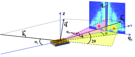
Figure 2: The scattering geometry w. r. to the reference axes fixed with the sample. A beam (X-ray/neutron) incidents at an angle $\alpha_{i}$ and gets scattered (reflected/diffracted) towards ($\alpha_{f},\phi$). $2\theta$ represents the deviation of the beam from its incident direction.

Fig. 2 shows a general scattering geometry when reference frame is chosen fixed with the sample. In this geometry, the incident wave vector is given by,

$$\overrightarrow{k_{i}}\doteq\frac{2\pi}{\lambda}\left(\begin{array}[]{ccc}cos\alpha_{i}\\ 0\\ -sin\alpha_{i}\end{array}\right)$$

and the scattered wave vector for an angle $\phi$ out-of the plane of reflection is given by,

$$\overrightarrow{k_{f}}\doteq\frac{2\pi}{\lambda}\left(\begin{array}[]{ccc}cos\alpha_{f}cos\phi\\ cos\alpha_{f}sin\phi\\ sin\alpha_{f}\end{array}\right)$$

where $\alpha_{i},\alpha_{f}$ are the incident and scattered angle w. r. to the sample. For elastic scattering, $|\overrightarrow{k_{i}}|=|\overrightarrow{k_{f}}|=k=\frac{2\pi}{\lambda}$. The transfer wave vector,

$$\overrightarrow{q}=\overrightarrow{k_{f}}-\overrightarrow{k_{i}}\doteq\frac{2\pi}{\lambda}\left(\begin{array}[]{ccc}cos\alpha_{f}cos\phi-cos\alpha_{i}\\ cos\alpha_{f}sin\phi\\ sin\alpha_{f}+sin\alpha_{i}\end{array}\right)$$ (10)

Using the relation

$$\widehat{k_{f}}\cdot\widehat{k_{i}}=cos2\theta=cos\alpha_{i}cos\alpha_{f}cos\phi-sin\alpha_{i}sin\alpha_{f}$$

one can obtain the following form for magnitude of the momentum transfer,

$$|\overrightarrow{q}|=q = \frac{2\pi}{\lambda}\sqrt{2[1-(cos\alpha_{i}cos\alpha_{f}cos\phi-sin\alpha_{i}sin\alpha_{f})]}$$ (11)

$$= \frac{2\pi}{\lambda}\sqrt{2(1-cos2\theta)}$$

$$= \frac{4\pi}{\lambda}sin\theta$$

Here, one may note that the last expression is equivalent to the Bragg’s condition for $d=\frac{2\pi}{q}=\frac{\lambda}{2sin\theta}$ where $2\theta$ is the deviation of the scattered beam from its initial direction. One important point is that the expression for $q_{z}$, derived from simple vector geometry becomes equivalent, apparently, with the Bragg’s condition which is essentially involved with interference! Actually, when one considers $d=\frac{2\pi}{q}$, the essence of interference effect automatically comes in as the $d-space$ is connected to the $q-space$ by Fourier transformation and vice-versa. Another point, obvious from the Bragg’s condition, $2dsin\theta=n\lambda$, is that when the small length-scale (atomic spacing of few Å) is probed, the Bragg peaks should appear at larger angles ($\theta\sim$ few tens of degrees) whereas for larger length-scales (few tens or hundreds of nm) the peaks should appear at smaller angles ($\theta\sim$ few degrees only) — the former one is the case of diffraction and the later for reflectivity.

Sometimes, it is convenient to express $\overrightarrow{q}$ in terms of the parallel (to sample surface) component, $q_{||}=\sqrt{q_{x}^{2}+q_{y}^{2}}$ and the perpendicular, $q_{\bot}=q_{z}$. The specular condition, $\alpha_{i}=\alpha_{f}=\theta$ with $\phi=0$, implies $q=q_{\bot}=q_{z}=2k_{z}=4\pi sin\theta/\lambda$. So specular reflectivity can be done either by varying $\lambda$ for fixed $\theta$ (energy resolved) or by varying $\theta$ for fixed $\lambda$ (angle resolved).

Footprint correction: One important correction needs to be included, particularly for specular reflectivity at small angles, when the footprint of the beam exceeds the sample size, L. If the beam width is W, then the footprint, F for an incidence angle of $\alpha_{i}$ is given by F=W/sin$\alpha_{i}$, hence, for F$>$L the experimental data need to be corrected by multiplying a factor of F/L.

Instrumental resolution: Another crucial point that one has to consider is the instrument resolution function. The effect of instrumental resolution can be considered as convolution by the resolution function which in most cases is approximated by a Gaussian whose standard deviation is usually determined by the full-width at half-maxima (FWHM) of the direct beam in a detector scan. We consider a Gaussian resolution function with suitably defined window [$\equiv$ (2 $\times$ N_resolution + 1) data points] for post-processing (weighted sum ) of the simulated data to include the instrumental resolution effect.

Specular reflectivity from liquid surface/interface:

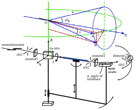
Figure 3: Schematic of the experimental set up and the beam geometry for reflectivity study from liquid surface. $\overrightarrow{OX}$ is the direct beam while OAX defines the horizontal plane. The rotation of the deflector crystal (black line at O) about the direct beam defines a cone of semi-opening angle $2\theta_{B}$ at O. The rotation of deflector crystal, $\chi$ is related to the angle of incidence, $\alpha$ through the relation $sin\alpha=sin(2\theta_{B})sin\chi$. To bring the point of interest back to its original position a vertically shift of $dtan\alpha$ followed by a horizontally rotation by an angle of $sin^{-1}[sin(2\theta_{B})(1-cos\chi)]$ is required.

While discussing about the scattering geometry and experimental set up for reflectivity study of solid samples, we may have a glimpse on the reflectivity study from liquid surface or liquid-liquid interface liquid1 which is special because the liquid surface necessarily be horizontal. Moreover, the reflected intensity from liquid surface/interface drops drastically with increase in angle hence a synchrotron beam is preferred. Unfortunately, synchrotron beams are usually fixed in direction and need to incline by Bragg-reflection using suitable single-crystal. Usually the deflector crystal is mounted at O,the center of the goniometer stage where the solid samples are mounted and the liquids are placed on an additional stage which can rotate about the vertical axis through O. The rotation of the deflector crystal about the direct beam ($\overrightarrow{OX}$, refer to Fig. 3) obeying the Bragg condition (for example, the Bragg angle of Ge($111$) at 18 keV $=\theta_{B}=6.008^{\circ}$) causes the Bragg-reflected beam to describe a cone of opening angle $4\theta_{B}$ ($\sqrt{z^{2}+y^{2}}=xtan(2\theta_{B})$). As a result, the change in angle of incidence causes the point of incidence to shift hence for each angle the point of incidence (the liquid stage as a whole) has to be brought back to its original position. Now, the locus of the beam on a virtual cylinder ($\sqrt{x^{2}+y^{2}}=d$: defined by the rotation of the liquid stage about the vertical axis through O) of radius d is given by $x^{2}[2-sec^{2}(2\theta_{B})]+2y^{2}+z^{2}=d^{2}$. If a rotation of the deflector crystal by an amount $\chi$ brings the horizontal beam $\overrightarrow{OA}$ to $\overrightarrow{OB}$ which makes an angle $\alpha$ with horizontal (x-y) plane then considering the vertical shift on a virtual vertical plane (not on the cylindrical surface), one can write, $dsin\alpha=dsin(2\theta_{B})sin\chi$ which relates the angle of incidence, $\alpha$ to the rotation of the crystal through the relation $sin\alpha=sin(2\theta_{B})sin\chi$. So, for a rotation of the deflector crystal by an amount of $\chi$, the point of interest should be vertically shifted by an amount of $dtan\alpha$ (for a line joining the origin and a point $\textbf{r}(x,y,z)$ that makes an angle $\alpha$ with x-y plane, it is obvious that $cos\alpha=z/r$ hence $tan\alpha=z/d$) followed by a horizontal rotation of $sin^{-1}[sin(2\theta_{B})(1-cos\chi)]$. To avoid the shifting of the incident spot while changing the incident angle two-crystal assembly may also be used where the fixed beam passes through one focus of an ellipsoid of revolution and the point of incidence on the liquid surface fixed at another focus while the driving crystals move in a coupled fashion over two circular cross-sections of the ellipsoid of revolution. However, using two crystals involves more loss of beam intensity and more complicity in alignment.

The dynamical theory and Parratt formalism:

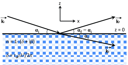
Figure 4: Schematic of reflection and refraction of a wave incident on a smooth surface at an angle $\alpha_{i}$. Reflected wave emerges at an angle, $\alpha_{f}=\alpha_{i}$ and the refracted wave transmitted through the medium at an angle $\alpha_{t}$. $\overrightarrow{k_{i}}$, $\overrightarrow{k_{f}}$, $\overrightarrow{k_{t}}$ are the incident, reflected and transmitted wave vectors, respectively.

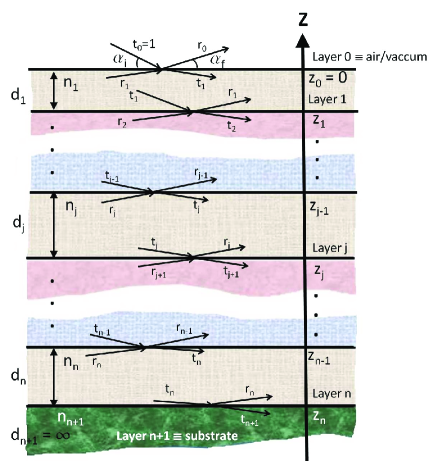
Figure 5: Schematic of multiple reflection from a multilayer film having $n$-layers on a substrate with $n+1$ interfaces. For incident wave amplitude is normalized to unity, $t_{0}=1$. No reflection from the substrate sets, $r_{n+1}=0$.

In classical treatment of scattering, the continuity of the electric and magnetic field vectors of the propagating electro-magnetic wave at an interface provides the relation between the reflection ($r$) and transmission ($t$) coefficients and hence imply the reflectivity, $R=r^{*}r$. For a smooth air-medium interface (refer to Fig. 4) with an incidence angle of $\alpha_{i}=\alpha_{f}$ (specular), the expression for $r$ and $t$, known as Fresnel formula is given by

$$r = \frac{k_{i,z}-k_{t,z}}{k_{i,z}+k_{t,z}},$$ (12)

$$t = \frac{2k_{i,z}}{k_{i,z}+k_{t,z}}$$ (13)

where

$$k_{i,z}=ksin\alpha_{i}$$

and (from Snell-Descartes’ law)

$$k_{t,z}=nksin\alpha_{t}=k\sqrt{n^{2}-cos^{2}\alpha_{i}}$$ (14)

The refracted wave transmits at an angle $\alpha_{t}$ through the medium having refractive index,

$$n=1-(\delta+i\beta)$$ (15)

where ED, $\rho$ is redefined as

$$\delta=r_{e}\rho\lambda^{2}/2\pi$$

and $\beta$ is the absorption co-efficient. It is more convenient to use $\rho$ (electron per ${\AA}^{3}$) rather than the dimensionless number $\delta$ because $\rho$ is a $\lambda$-independent specific number for a material. The dynamical calculation, for a thin film consisting of a single layer on a substrate, using matrix transfer method gibaud ; tolan for each layer which essentially connects the fields between two consecutive layers, yields the following relation

$$r = \frac{r_{0,1}+r_{1,2}e^{-2ik_{z,1}}}{1+r_{0,1}r_{1,2}e^{-2ik_{z,1}}}$$ (16)

$$t = \frac{t_{0,1}t_{1,2}e^{-ik_{z,1}}}{1+r_{0,1}r_{1,2}e^{-2ik_{z,1}}}$$ (17)

where $r_{j,j+1}$ is the coefficient of reflection at the interface between $j$-th and $(j+1)$-th layer. It may be noted here that the additive term to unity in the denominator corresponds to multiple reflection in the film. Extension to a multi-layer film having $n$ homogeneous layers on a substrate, one obtains the recursion relation for the ratio of reflection and transmission coefficients of the j-th layer, as follows

$$X_{j}=\frac{r_{j}}{t_{j}}=e^{-iq_{z,j}z_{j}}\frac{r_{j,j+1}+X_{j+1}e^{(iq_{z,j+1}z_{j})}}{1+r_{j,j+1}X_{j+1}e^{(iq_{z,j+1}z_{j})}}$$ (18)

where $q_{z,j}=2k_{z,j}$ and $z_{j}=\sum_{m=0}^{j}d_{m}\equiv$ depth including the j-th layer thickness from top. In our convention (refer to Fig. 5), $j=0$ for air/vacuum and $j=n+1$ for the substrate. The expression for $r_{j,j+1}$ is given by

$$r_{j,j+1}=\frac{q_{z,j}-q_{z,j+1}}{q_{z,j}+q_{z,j+1}}$$ (19)

with

$$q_{z,j} = \sqrt{{q_{z}}^{2}-\frac{32\pi^{2}}{\lambda^{2}}(\delta_{j}+i\beta_{j})}$$ (20)

$$= \sqrt{{q_{z}}^{2}-16\pi r_{e}\rho_{j}-\frac{i32\pi^{2}\beta_{j}}{\lambda^{2}}}$$ (21)

No reflection from the substrate (assumed to be sufficiently thick) sets

$$X_{n+1}=0$$

as the start of the recursion. After $n+1$ iterations, the expression for specular reflectivity is obtained as

$$R=|X_{0}|^{2}$$

Critical Angle: It may be noted here that, X-ray, propagating through a medium of higher refractive index, suffers total external reflections when incident on a surface of a material having lower refractive index. The very concept of total external angle defines an angle below which the X-rays are totally reflected back and termed as Critical angle. Setting $\alpha_{t}=0$ in eqn. (14), one obtains $n^{2}(\approx 1-2\delta)=cos^{2}\alpha_{c}(\approx 1-\alpha^{2}_{c})$ i.e. the critical angle, $\alpha_{c}$ is related to the ED of the material as

$$\alpha_{c}\approx\sqrt{2\delta}=\lambda\sqrt{r_{e}\rho/\pi}=sin^{-1}(\lambda q_{c}/4\pi)$$ (22)

Typical orders of magnitude are: $\delta\simeq 10^{-5}$ and $\beta\simeq 10^{-6}$ so that $\alpha_{c}\simeq 0.1^{\circ}$ to $0.5^{\circ}$. For Si, $\delta_{Si}=7.6\times 10^{-6}$ and corresponding $\alpha_{c}=0.223^{\circ}$ with $q_{c}=0.0316$ Å^-1 for $\lambda=1.54$ Å. For a multilayer film, the overall critical angle is determined by the layer having the highest value of $\delta$. In Fig. 1, the critical angle for blue curve (Au on Si) is defined by $\delta_{Au}$ as $\delta_{Au}=4.96\times 10^{-5}>\delta_{Si}$ whereas for red curve (PS on Si) the critical angle is defined by $\delta_{Si}$ as $\delta_{Si}>\delta_{PS}=3.5\times 10^{-6}$. For incident angle less than the critical angle i.e. $\alpha_{i}<\alpha_{c}$, the penetration depth is only few nano-meters, however, it increases sharply to several micro-meters as $\alpha_{i}$ exceeds $\alpha_{c}$ and X-ray immediately sees the whole layer. Actually, there is a so-called evanescent wave within the refracting medium, propagating parallel to the interface and exponentially decaying perpendicular to it. In grazing incidence diffraction (GID) study where only the first few atomic layers are of main interest $\alpha_{i}$ is kept just below the $\alpha_{c}$ i.e. ($\alpha_{i}\lesssim\alpha_{c}$).

The transfer matrix formalism is equivalent to the recursive approach of Parratt’s parratt ; gibaud ; tolan formalism and both (known as Dynamical Theory) are fairly exact since it incorporates the issue of multiple scattering. The additive term to unity in the denominator of eqn. (18), corresponding to multiplicative reflection gibaud ; tolan , contributes significantly for small incident angles and when ignored the reflectivity expression can be simplified to,

$$R(q_{z}) = \left|\sum_{j=0}^{n}r_{j,j+1}e^{i\sum_{m=0}^{j}q_{z,m}d_{m}}\right|^{2}$$ (23)

$$= \left|\sum_{j=0}^{n}\frac{q_{z,j}-q_{z,j+1}}{q_{z,j}+q_{z,j+1}}e^{i\sum_{m=0}^{j}q_{z,m}d_{m}}\right|^{2}$$

where $d_{j}$ is the thickness of $j$-th layer.

In further assumption that the incident angle does not change significantly from layer to layer i.e. $q_{z}$ is same for all layers, with an additional approximation (so that first two terms of the binomial expansion of the right hand side of the eqn. (21) would be sufficient to consider),

$$q_{z}>q_{c}=\frac{4\pi}{\lambda}sin\theta_{c}=\sqrt{16\pi r_{e}\rho}$$ (24)

one can write eqn. (23) in a simpler form:

$$R(q_{z}) = \frac{64\pi^{4}}{\lambda^{4}q^{4}_{z}}\left|\sum_{j=0}^{n}({\delta_{j+1}-\delta_{j}})e^{iq_{z}z_{j}}\right|^{2}$$ (25)

$$= \frac{(4\pi r_{e})^{2}}{q_{z}^{4}}\left|\sum_{j=0}^{n}({\rho_{j+1}-\rho_{j}})e^{iq_{z}z_{j}}\right|^{2}$$ (26)

where $\sum_{m=0}^{j}d_{m}=z_{j}\equiv$ depth including the j-th layer thickness from top. Eqn. (26) is exactly the same with eqn. (1) in the continuous limit. This greatly simplified treatment, known as the Kinematical Theory or Born approximation reduces the Parratt recursive formula to a simple relation.

In Born approximation, the effect of multiple reflection from different layers of a multi-layer film is ignored and also the effect of refraction from one layer to another is not considered by assuming the incident angles to be same for all interfaces. Hence, for a bare substrate where there is no multiple reflection and only one angle of incidence, both the Parratt curve and the Born curve are expected to be identical and same with the Fresnel curve. However, the third approximation (24) makes the difference and fails to restrict the Born curve from blowing up at small angles.

Formulation of reflectivity expression for scattering of electromagnetic wave from rough surfaces is difficult as the solution of the relevant wave equations turns out to be complicated involving matching of the boundary conditions over random rough surfaces and several simplifying assumptions have to be invoked for their solution. An exponential damping factor may be included when the roughness ($\sigma$) has an error-function profile, as introduced by Névot and Croce gibaud ; tolan to modify eqn. (19), eqn. (23) and eqn. (26) in the following form:

$$r_{j,j+1}=\frac{q_{z,j}-q_{z,j+1}}{q_{z,j}+q_{z,j+1}}e^{-\frac{q_{z,j}q_{z,j+1}\sigma^{2}_{j,j+1}}{2}}$$ (27)

$$R(q_{z})=\left|\sum_{j=0}^{n}\frac{q_{z,j}-q_{z,j+1}}{q_{z,j}+q_{z,j+1}}e^{i\sum_{m=0}^{j}q_{z,m}d_{m}}e^{-\frac{q_{z,j}q_{z,j+1}\sigma^{2}_{j,j+1}}{2}}\right|^{2}$$ (28)

$$R(q_{z}) = \frac{64\pi^{4}}{\lambda^{4}q^{4}_{z}}\left|\sum_{j=0}^{n}({\delta_{j+1}-\delta_{j}})e^{iq_{z}z_{j}}e^{-\frac{q_{z}^{2}\sigma^{2}_{j,j+1}}{2}}\right|^{2}$$ (29)

$$= \frac{(4\pi r_{e})^{2}}{q_{z}^{4}}\left|\sum_{j=0}^{n}({\rho_{j+1}-\rho_{j}})e^{iq_{z}z_{j}}e^{-\frac{q_{z}^{2}\sigma^{2}_{j,j+1}}{2}}\right|^{2}$$ (30)

It may be noted here that the roughness term as introduce here carries more weightage for larger $q_{z}$ hence damps the reflectivity curve slightly more in comparison with roughness introduced following eqn. (LABEL:rough).

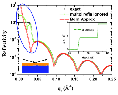
Figure 6: Reflectivity curves for a 100 Å thick single layer of PS on Si substrate following different formalism. Electron density, convoluted with the roughness is in the inset. The region highlighted by the blue circle shows distinct difference between the curves. The back one is for exact dynamical theory. The effect of multiple reflection is ignored for green curve. Further approximation (Born) that the incident angle to be same at all interfaces and $q_{z}>q_{c}$ is assumed for the red curve.

Fig. 6 compares the reflectivity curves for a 100 Å thick single layer of PS on Si substrate following eqn. (18) using (27), (28) and (30). The inset figure shows the electron density profile with the gaussian roughness (refer to eqn. (LABEL:rough)) of the interfaces. The region highlighted by the blue circle, particularly around $q_{c}^{Si}=0.0316$ Å^-1, shows distinct difference between the curves. The back one is for exact dynamical theory. The effect of multiple reflection causes the reflectivity to grow more than 1 as observed for the green curve. For the Born approximated (blue) curve, the deviation is even serious as it assumes further that the incident angle to be the same at all boundaries.
Polarized neutron reflectivity (PNR): In addition to the structural information, reflectivity study using the spin polarized neutron (PNR) provides the detail of in-plane magnetic ordering in a magnetic thin film. Neutrons arriving at the sample surface are spin polarized either parallel $(+)$ or antiparallel $(-)$ to the quantization axis defined by the applied magnetic field, H (along the y-direction, refer to Fig. 2). In this case, the refractive index includes the nuclear and magnetic scattering contributions and expressed as

$$n^{\pm}(z)=1-(b\mp c\mu)$$ (31)

where $b$ is the complex nuclear SLD and $c=\lambda^{2}m_{n}\mathbf{\mu}_{n}/\hbar^{2}$ and $\mathbf{\mu}(\mu_{x},\mu_{y},\mu_{z})$ is the magnetization. Eqn. (31) is same, except the additional magnetic term, with eqn. (15) as $b\equiv\delta+i\beta$. Depending upon the polarization of incident and reflected neutron beam, the measured reflectivities are designated as $R^{++}$, $R^{--}$, $R^{+-}$ and $R^{-+}$. The non-spin-flip (NSF) data, $R^{++}$ and $R^{--}$ depend on structural as well as magnetic contribution and provide the magnetization parallel to the applied field [($R^{++}-R^{--})\propto<\mu_{y}>$], however, the spin-flip (SF) intensities, $R^{+-}$ and $R^{-+}$ reflectivities (usually, these two are degenerate) are purely of magnetic origin and depend on the average square of the transverse in-plane magnetic moment, $<\mu_{x}^{2}>$ zabel ; sg . One important feature of PNR is that the value obtained for $<\mu_{y}>$ can be calibrated in $\mu_{B}$ units because the number of scatterer can be estimated from simultaneous analysis of R⁺⁺ and R^– using Eq. (31). The PNR data, collected in this geometry, are insensitive to the out-of-plane moment $\mu_{z}$. In PNR study of antiferromagnetic thin-films, one obtains additional half-order peaks corresponding to double the lattice spacing in real space of similar spins.
Comparison between X-ray and neutron refractivities: The nature of interaction for X-ray and neutron with the scatterer is different as X-ray sees the electron cloud within the sample (long-range electro-magnetic interaction) but neutron sees the nucleuses as point scatterer (short-range strong interaction) in addition with the magnetic (long-range electro-magnetic) structure of the scatterer (in case of polarized neutron reflectivity utilizing the intrinsic dipole moment of neutrons). Even with laboratory-sources of X-ray, the reflectivity as low as $10^{-8}$ and $q_{z}$ value as high as $\simeq$1 Å^-1 can be achieved, however for neutron reflectivity, it is difficult to have $R$ values below $10^{-6}$ or $q_{z}$ beyond 0.2 Å^-1. Unlike monotonic dependence of electron density over atomic number in case of X-ray, the neutron reflectivity provides reacher structure since the scattering length density varies drastically from element to element even for different isotopes of the same atom and can be negative as well.

Auto-correlation function and the phase problem:
Here, we discuss the difficulty of finding unique ED profile from reflectivity data. As the reflectivity expression is obtained as modulus-squared in the final step, the information of the phase of the scattered wave is lost in the reflectivity experiments as a result the direct inversion of the data to reconstruct the EDP is impossible. However, supplemented with additional information like prior knowledge of number of layers etc. from sample preparation makes it possible to extract the EDP.

Now let us discuss the lack of uniqueness of EDP mathematically by considering the auto-correlation function or ACF of $f(z)$, which provides a model-independent real-space representation of the information contained in the intensity of reflectivity pattern, defined as,

$$ACF(z)=\int_{-\infty}^{\infty}f(t)^{*}f(z+t)dt=\int_{-\infty}^{\infty}|F(q)|^{2}e^{izq}dq$$ (32)

where $F(q)$ is the FT of $f(z)$. Considering $d\rho/dz=\rho^{\prime}(z)\equiv f(z)$ and comparing eqn. (32) with eqn. (3), one can write, the ACF of $\rho^{\prime}(z)$ as follows:

$$ACF(\rho^{\prime}(z))=\mathcal{F}^{-1}\left[\frac{\rho_{s}^{2}R(q_{z})}{R_{F}(q_{z})}\right]=\mathcal{F}^{-1}\left[\mathfrak{R}(q_{z})\right]$$ (33)

where $\mathcal{F}^{-1}$ is the inverse FT and $\mathfrak{R}(q_{z})=\frac{\rho_{s}^{2}R(q_{z})}{R_{F}(q_{z})}$. The above expression is known as the Patterson function and imply the information regarding the depth of interfaces independent of any model. However, there is an inherent discrepancy of this data inversion technique due to the so-called phase-loss ambiguity. As a result some peaks may get introduced additionally or get overlooked in the ACF of $\rho^{\prime}(z)$ as pair-wise depth difference does matter in its calculation. A pair of sharp peaks, say, at $z_{1}$ and $z_{2}$ with amplitudes $A_{1}$ and $A_{2}$, respectively, contributes to a symmetric pair of very sharp peaks at $\pm(z_{1}-z_{2})$ with amplitude $A_{1}A_{2}$ to $ACF(z)$ along with an additive of $A^{2}_{1}+A^{2}_{2}$ to the ACF at the origin. For $n$ interfaces i.e. $n$ number of peak in $\rho^{\prime}(z)$ will pair-wise contribute to $n(n-1)$ number of peaks towards its ACF in general. The peak for air-sample interface at $z=0$ in $\rho^{\prime}(z)$, when considered pair-wise with other interfaces, will contribute to $(n-1)$ peaks at their respective positions. But, the additional peaks with the possibility of overlap and/or exact cancelation may complicate the analysis unless one has prior information of layers from sample growth.

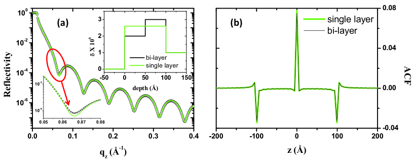
Figure 7: (a) A particular combination of thicknesses and EDs may result in similar reflectivity curves when corresponding ACFs are the same. The reflectivity curves for a bi-layer and a single layer film of same total thickness of 100 Å on the same substrate look alike. The ED is shown in the inset and small deviation near the first deep is magnified for clarity. (b) The corresponding ACFs or the Patterson functions are the same in both cases.

As for example, let us consider two x-ray reflectivity curves looking exactly the same except a small difference near the first deep, marked by the red circle in Fig. 7a. The black curve corresponds to a bi-layer film ($\delta_{1}=2\times 10^{-6}$ and $\delta_{2}=3\times 10^{-6}$) having same thickness of 50 Å each on a substrate ($\delta_{s}=1\times 10^{-6}$). For green curve, there is only a single layer ($\delta=2.6\times 10^{-6}$) of thickness 100 Å on the same substrate. At $z=\pm 50$ Å, exact cancelation of the contributions from pairs of $\delta$-functions at ($z=0$; $z=50$ Å) and ($z=50$ Å; $z=100$ Å) in case of the bi-layer film results in the same ACF as for single layer, and hence both reflectivity curves look exactly the same (refer to Fig. 7b)! Interestingly, such situation may happen when $\delta_{1}=\sqrt{\delta(\delta-\delta_{s})}=\delta_{2}-\delta_{s}$ where $\delta_{2}>\delta>\delta_{1}>\delta_{s}$.

To generate the ACF, one may directly use the discrete inverse FT formula given by,

$$ACF(z)=\frac{1}{N}\sum_{k=0}^{N-1}\mathfrak{R}(q_{k})e^{-iq_{k}k}$$ (34)

where $k=0,1,2,....,N-1$ which needs the $\mathfrak{R}(q_{z})$ to be defined from $q_{min}=0$ with uniform $\delta q_{z}$ and the obtained ACF will be automatically scaled having uniform interval of unity ($\delta z=1$). However, the truncation effect due to finite span or window of $q_{z}$ which introduces ripples in the ACF with a characteristic wavelength of $2/q_{max}$ will be unavoidable. The peaks in ACF will be distinct and better when $q_{max}$ as large as $\pi$ and larger the number of data points. When a standard inverse FT tool is used, it is convenient to interpolate the reflectivity data from $q_{min}=0$ to $q_{max}=\pi$ with uniform $\delta q=\pi/N$ so that ACF (exchanging the positive half and the negative half) will be automatically scaled with unit interval between $\pm N$.

Data inversion technique: A direct data inversion is cumbersome due to many practical difficulties like limited extent of measured value of $q_{z}$, statistical noise, incoherent background signal and the blurring from instrumental resolution.
Having preliminary idea about the system one can simulate the reflectivity curve close enough to the experimental one by proper choice of parameters. For a close choice of model EDP $\rho_{m}(z)$ with corresponding simulated reflectivity, $R_{m}(q_{z})$ one may start iterationfitmilan using the following ansatz

$$\rho_{e}^{\prime}(z)=\mathcal{F}^{-1}\left[\sqrt{\frac{R_{e}(q_{z})}{R_{m}(q_{z})}}\mathcal{F}[\rho_{m}^{\prime}(z)]\right]$$

where $R_{e}(q_{z})$ is the experimental reflectivity and $\rho^{\prime}_{e}(z)$ is used as the $\rho^{\prime}_{m}(z)$ in the next iteration.

III LabVIEW-based versatile reflectivity simulator:

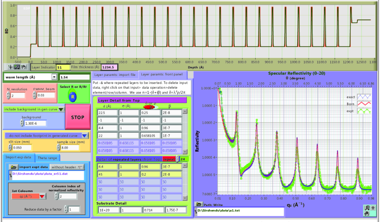
Figure 8: Front panel of the developed specular reflectivity simulator using LabVIEW (version $8.5$). The programme simultaneously generates reflectivity curves for a multilayer thin film following Born approximation (red curve) as well as the exact dynamical theory according to the range and steps of the imported experimental data (green) or as provided from the front panel for model parameters (thickness, roughness, ED, absorption coefficient) fed from the front panel or from parameter file (.txt or .dat having four coloumns with headers for thickness, roughness, delta and beta, respectively) providing the path.

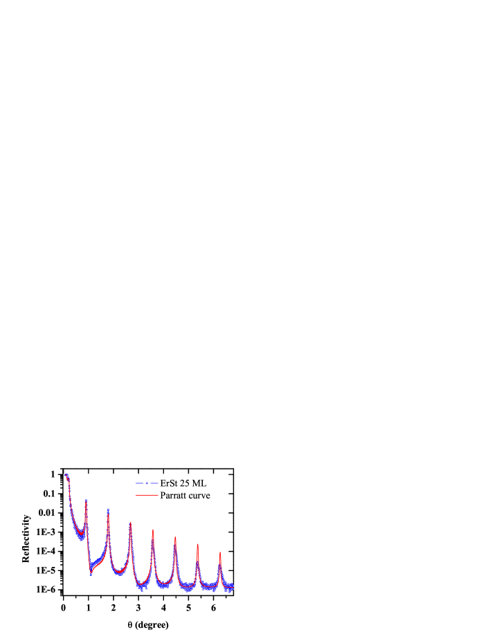
Figure 9: The specular reflectivity curve (blue dots) of stacked multi-layer of erbium stearate LB film on Si substrate. The red line is the generated curve following the Parratt formalism.

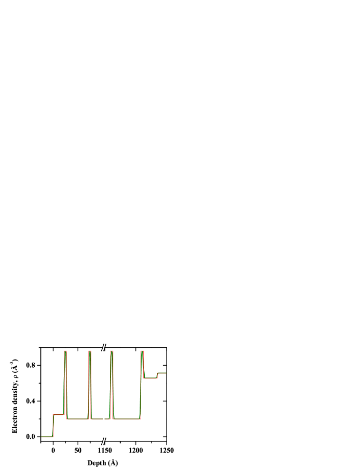
Figure 10: Variation of electron density along the depth [from air (z = 0) to substrate] of an erbium stearate LB film (having 25 repetition of Er⁺ layers, each separated by a hydrocarbon-tail) on Si substrate with (dark green) and without (red) roughness (Gaussian) effect.

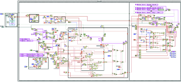
Figure 11: Block diagram or the source code of the developed specular reflectivity simulator using LabVIEW. Different icons corresponding to different logical operations, connected through wires through which data flow.

Fig. 11 shows the block diagram of the simulator. The code is build by drag-n-drop the icons and connecting them by wires through which data flow following the desired logic. One can easily modify and customize any of such programmes according to their need and preferences.

Fig. 8 shows the screen-shot of the front panel of the simulator which simultaneously plots specular reflectivity curves for a multi-layer film following the (i) exact dynamical theory (eqn. (18) with eqn. (27)) and the (ii) Born Theory (eqn. (30) with restriction $R\leq 1$) according to the range and steps of the imported experimental data (normalised) or as provided from the front panel corresponding to the model parameters (thickness, roughness, ED, absorption coefficient) fed from front panel or imported from file providing the path. The simulator needs the followings as the input: wavelength ($\lambda$) in Å or energy in keV, range and step of $\theta$ (or according to the experimental data when imported, providing the path), layer detail i.e. $d,\sigma,\delta,\beta$ (with option to be imported, providing the path), FWHM of the direct beam, number of data point (N_resolution) to define the instrumental resolution window and the output path. It is easy to include repeated layers by just putting $-1$ for $d,\sigma,\delta,\beta$ to a particular layer where the repeated layers are intended to be inserted. The repeated layer detail with number of repeat can be incorporated in another window of the front panel. To delete input data, one has to right click on that particular input $>$ data operation $>$ delete element$/$row$/$column. Inclusion of background and footprint effect (providing the sample size and beam width) are optional. $R$ (or $R/R_{F}$ as selected) vs. $q_{z}$ and $R$ (or $R/R_{F}$ as selected) vs. $\theta$ along with the electron density profile (EDP) including the roughness modification are simultaneously plotted during run as shown in Fig. 8. The total thickness of the film and the number of layers in between air and substrate is displayed in the front panel during run. The simulator generates five output files, namely, the parameter file (filenamepar.txt), box EDP (filename_boxEDP.txt) and the convoluted EDP (filename_convEDP.txt), the simulation data file with (filename_generated.txt) and without (filename.txt) inclusion of the instrumental resolution effect. While simulating the reflectivity curve for an experiential data, one can reduce the simulation time using the option of reducing the number of data points by a given factor.

A typical reflectivity data (refer to Fig. 9) of a multi-layer of erbium stearate Langmuir-Blodgett film on Si substrate obtained from a lab-source (rotating copper anode, Enraf Nonius, model FR591) using Cu$\alpha$ characteristic X-ray is considered here to estimate the parameters by simulating the reflectivity curve. In the out-of-plane direction, the film consists of 25 layers of Er separated by organic spacer (stearate tail). The thickness of different layers from the top (i.e. from air to substrate), used to simulate the curve is as follows: stearate tail (22.5 Å) + 24 $\times$ [Er⁺-head (4.4 Å) + stearate tail (45 Å)] + Er⁺-head (4.4 Å] + SiO₂ (22 Å). The total film-thickness is 1234.5 Å and total number of model-layers is 51. Corresponding electron density profile with and without the roughness effect is shown in Fig. 10.

Once having a close guess of the parameters, experimental data can be fitted utilizing LabVIEW platform with constrained non-linear least-square fit option using the Levenberg-Marquardt algorithm or the trust-region dog-leg algorithm to optimize the set of parameters for the best fit. LabVIEW-based fitting part is in progress. A model-independent ACF or the Patterson function generation programme from the specular reflectivity data which provides an idea about the thickness of layers and the depth of interfaces is also developed. Some programmes are also developed those are useful in furnishing the spec-files. It may be mentioned here that the stand-alone executable version of the simulator is also built and it needs only the LabVIEW run-time environment (free to download from National Instruments).

Download link: One needs to run the main programme specular reflectivity simulator.vi only, however, it needs two sub-programmes namely, boxEDP_subVI.vi and convEDP_subVI.vi (to be placed in the same folder) during run. Click here to download the zipped folder containing these three programme and other related programme files. One may use the stand-alone version reflgen.exe as well. Without having full Labview software, one needs to install only the LabVIEW run-time engine (free to download from National Instruments). The limitation of this version is that the source code i.e. the block diagram is not available hence can not be edited. After downloading one should run it to open the actual Labview simulator. From File $>$ VI properties, one can find the location of the programme to copy and paste it at the desired folder. The programme named BornReflGen_ACF can be used to generate the Born reflectivity and corresponding ACF. To merge reflectivity data, furnish spec-files and for conversion of electron density, the other programmes may be helpful.

References

- (1) L. G. Parratt, Phys. Rev. 95, 359 (1954).
- (2) T. P. Russell, Mat. Sc. Rep. 5, 171 (1990).
- (3) J. Daillant and A. Gibaud, X-ray and neutron reflectivity : principle and applications, Lectures notes in physics (Springer, 1999).
- (4) M. Tolan, X-ray scattering from soft-matter thin films, 5-89 (Springer, 1999).
- (5) J. Als-Nielsen and D. McMorrow, Elements of modern X-ray physics, 61-95 (John Wiley & Sons, 2001)
- (6) J. K. Basu and M. K. Sanyal, Phys. Rep. 363, 1 (2002).
- (7) V. A. Kheraj, C. J. Panchal, M. S. Desai and V. Potbhare, Pramana: J. Phys. 72, 1011 (2009).
- (8) D. S. Sivia, Elementary scattering theory: for X-ray and neutron users, 93-112 (Oxford, 2011).
- (9) M. L. Schlossman et. al, Rev. Sci. Instrum. 68, 4372 (1997).
- (10) M. K. Sanyal, S. Hazra, J. K. Basu, and A. Datta, Phys. Rev. B 58, R4258 (1998).
- (11) H. Zabel, K. Theis-Bröhl, and B.P. Toperverg, The Handbook of Magnetism and Advanced Magnetic Materials: Vol. 3 - Novel Techniques, H. Kronmüller, S.P.S. Parkin (Eds.), 2327 - 2362, (Wiley, New York, 2007).
- (12) S. Gayen, M. K. Sanyal, A. Sarma, M. Wolff, K. Zhernenkov, and H. Zabel, Phys. Rev. B 82, 174429 (2010).