Fast and robust population transfer in two-level quantum systems with dephasing noise and/or systematic frequency errors

Abstract

We design, by invariant-based inverse engineering, driving fields that invert the population of a two-level atom in a given time, robustly with respect to dephasing noise and/or systematic frequency shifts. Without imposing constraints, optimal protocols are insensitive to the perturbations but need an infinite energy. For a constrained value of the Rabi frequency, a flat $\pi$ pulse is the least sensitive protocol to phase noise but not to systematic frequency shifts, for which we describe and optimize a family of protocols.

I Introduction

The coherent manipulation of quantum systems with time-dependent interacting fields is a major goal in atomic, molecular and optical physics, as well as in solid-state devices, for fundamental studies, Nuclear Magnetic Resonance and other spectroscopic techniques, metrology, interferometry, or quantum information applications Allen ; Bergmann ; Vitanov-Rev1 ; Kral ; Molmer ; Guerin . Two-level systems are ubiquitous in these areas, and the driving of a population inversion is an important operation that should be typically fast, faithful, stable with respect to different types of noise and perturbations, and of course “feasible in practice”. The later requirement depends on the specific system but may be sensibly quantified by setting constraints on the possible values of the control parameters. These constraints imply quantum speed limits that could be satisfied by optimized protocols.

In a recent paper Andreas , the stability of fast population inversion protocols with respect to amplitude noise and to systematic perturbations of the driving field was studied, and optimally stable protocols were found by making use of invariant-based inverse engineering and perturbation theory. Our aim here is to extend the analysis to dephasing noise, which may be the dominant source of decoherence due to environmental effects or the randomly fluctuating frequency of the control field, and to systematic frequency errors. By “systematic error” we mean here a constant shift of the frequency with respect to the one in the ideal protocol, due e.g. to calibration imperfections or inhomogeneous broadening.

We shall make use, as in Andreas ; ChenPRA , of invariant-based inverse-engineering, which is summarized in Sec. II. Section III describes the system and the perturbations by a Lindblad master equation. Perturbation theory is then used in Sec. IV to derive an expression for the sensitivity of population inversion with respect to dephasing noise or systematic frequency errors, and optimal protocols are defined with or without constraints. Section V deals with systematic frequency errors and, finally, both types of perturbation – due to the dephasing noise and constant frequency offset – are combined in Sec. VI. We shall for concreteness use a language appropriate for two-level atoms in optical fields, but the results are applicable to other two-level quantum systems.

II Shortcuts to adiabaticity

II.1 Dynamical invariants

We consider a two-level quantum system driven by a time-dependent Hamiltonian of the form

$$H_{0}(t)=\frac{\hbar}{2}\left(\begin{array}[]{cc}-\Delta(t)&\Omega(t)\\ \Omega(t)&\Delta(t)\\ \end{array}\right),$$ (1)

in the basis $|1\rangle={1\choose 0}$, $|2\rangle={0\choose 1}$. Eq. (1) corresponds to a laser-adapted interaction picture, where the rapid oscillations of the field have been transformed out, and $\Delta(t)$ and $\Omega(t)$ are the time-dependent detuning and (real) Rabi frequencies. Associated with this time-dependent Hamiltonian there are Hermitian dynamical invariants $I(t)$, fulfilling $\partial I/\partial t+(1/i\hbar)[I,H_{0}]=0$, so that their expectation values remain constant. $I(t)$ may be parameterized as ChenPRA ; spinQD

$$I(t)=\frac{\hbar}{2}\Omega_{0}\left(\begin{array}[]{cc}\cos\theta&\sin\theta e^{-i\beta}\\ \sin\theta e^{i\beta}&-\cos\theta\end{array}\right),$$ (2)

where $\Omega_{0}$ is an arbitrary constant (angular) frequency to keep $I(t)$ with dimensions of energy, and $\theta\equiv\theta(t)$ and $\beta\equiv\beta(t)$ are time dependent angles. Using the invariance condition we find the differential equations

$$\dot{\theta}(t) = -\Omega(t)\sin\beta(t),$$ (3)

$$\dot{\beta}(t) = -\Omega(t)\cot\theta(t)\cos\beta(t)-\Delta(t).$$ (4)

The eigenstates of the invariant $I(t)$, satisfy $I(t)|\phi_{n}(t)\rangle=\lambda_{n}|\phi_{n}(t)\rangle$ ($n=\pm;\lambda_{\pm}=\pm\hbar\Omega_{0}/2$). Consistently with orthogonality and normalization they can be written as

$$|\phi_{+}(t)\rangle=\left(\begin{array}[]{c}\cos\frac{\theta}{2}e^{-i\beta}\\ \sin\frac{\theta}{2}\end{array}\right),|\phi_{-}(t)\rangle=\left(\begin{array}[]{c}\sin\frac{\theta}{2}\\ -\cos\frac{\theta}{2}e^{i\beta}\end{array}\right).$$ (9)

According to Lewis-Riesenfeld theory LR , the solution of the time-dependent Schrödinger equation, up to a (global) phase factor, can be expressed as

$$|\Psi(t)\rangle=\Sigma_{n}c_{n}e^{i\gamma_{n}(t)}|\phi_{n}(t)\rangle,$$ (10)

where the $c_{n}$ are time-independent amplitudes, and the $\gamma_{n}(t)$ are Lewis-Riesenfeld phases

$$\gamma_{n}(t)\equiv\frac{1}{\hbar}\int_{0}^{t}\langle\phi_{n}(t^{\prime})|i\hbar\frac{\partial}{\partial t^{\prime}}-H_{0}(t^{\prime})|\phi_{n}(t^{\prime})\rangle dt^{\prime},$$ (11)

where the initial time $t_{i}$ has been chosen as $t_{i}=0$. In our two-level system model, the Lewis-Riesenfeld phases take the form

$$\gamma_{\pm}(t)=\pm\frac{1}{2}\int_{0}^{t}\left(\dot{\beta}+\frac{\dot{\theta}\cot\beta}{\sin\theta}\right)dt^{\prime}.$$ (12)

II.2 Inverse engineering

We shall now review briefly the inverse engineering of population inversion based on dynamical invariants. The initial and final states of the process are set as $|\Psi(0)\rangle=|2{\rangle}\equiv$$0\choose 1$ and $|\Psi(T)\rangle=|1{\rangle}\equiv$$1\choose 0$ respectively. The state trajectory between them may be parameterized according to one of the eigenstates, $|\phi_{n}(t)\rangle$, of the invariant. By using $|\phi_{+}(t)\rangle$ in Eq. (9), the boundary conditions ChenPRA

$$\theta(0)=\pi,~{}~{}~{}\theta(T)=0,$$ (13)

guarantee the desired initial and final states. If in addition

$$\dot{\theta}(0)=0,~{}~{}~{}\dot{\theta}(T)=0,$$ (14)

then $\Omega(0)=\Omega(T)=0$, and $H_{0}(t)$ and $I(t)$ commute at times $t=0$ and $t=T$. Apart from the boundary conditions, $\theta(t)$ and $\beta(t)$ are in principle quite arbitrary, and the possible divergences at multiples of $\pi$ of $\beta$ may be canceled with a vanishing $\dot{\theta}$. The commutativity at the time boundaries implies that the operators share the eigenstates so, if $H_{0}(t)$ remains constant before and after the process time interval $[0,T]$, then the initial eigenstates of $H_{0}(t<0)$ will be smoothly inverted into final eigenstates of $H_{0}(t>T)$ following the invariant eigenvectors. If the condition (14) is not imposed, the states at $t=0$ and $t=T$ will not be stable (stationary eigenstates), so a sudden jump is required in the Hamiltonian to make them so. The flat $\pi$ pulse is a clear simple example, where the Rabi frequency jumps from or drops to zero abruptly. Once $\theta(t)$ and $\beta(t)$ have been specified (the interpolation may be based on simplicity or to satisfy further conditions) the Rabi frequency and detuning are given, from Eqs. (3) and (4), by

$$\Omega(t) = -\frac{\dot{\theta}(t)}{\sin\beta(t)},$$ (15)

$$\Delta(t) = \dot{\theta}(t)\cot\beta(t)\cot\theta(t)-\dot{\beta}(t).$$ (16)

For $\beta(t)=\pi/2$, then $\Delta=0$, and

$$\int^{T}_{0}\Omega(t)\,dt=\pi$$ (17)

corresponds to a $\pi$ pulse. In particular, for $|\dot{\theta}|=\pi/T$, the flat $\pi$ pulse ($\Omega(t)=\pi/T$ and $\Delta=0$) minimizes, for a given $T$, the maximal value of $\Omega(t)$ along the protocol, $\Omega^{\rm max}=\mbox{max}_{t}|\Omega(t)|$.

III Model for dephasing noise and systematic frequency shifts

We assume that the dynamics of the two-level quantum system with dephasing noise and systematic error may be described by a master equation in Lindblad form book ; Lindblad ,

$$\frac{\partial\rho}{\partial t}=-\frac{i}{\hbar}[H_{0}+H_{1},\rho]-\frac{1}{2}(\Gamma_{d}^{{\dagger}}\Gamma_{d}\rho+\rho\Gamma_{d}^{{\dagger}}\Gamma_{d}-2\Gamma_{d}\rho\Gamma_{d}^{{\dagger}}),$$ (18)

where $\rho$ is the density matrix, $H_{0}$ is the unperturbed Hamiltonian (1), $H_{1}=\hbar\delta_{0}\sigma_{z}/2$ describes the systematic frequency error ($\delta_{0}$ is a constant frequency shift), $\Gamma_{d}=\gamma_{d}\sigma_{z}$ is the Lindblad operator corresponding to a dephasing rate $2\gamma_{d}^{2}$ Sarandy07 , and $\sigma_{z}$ is the $z$ Pauli matrix. This master equation results from averaging over white noise realizations of the fluctuation of the laser frequency or more generally, of the detuning, see the appendix in Andreas . The designed detuning thus may generally be perturbed in our model by a systematic constant offset and a random contribution with zero mean and delta-function correlation function. The dephasing effect corresponds to the randomization of the relative phases of coherent superpositions of states. It is detrimental for a process of complete population transfer, since the dynamics goes necessarily through a transient superposition of states. Very few analytic solutions are known for such systems (see for instance Kyoseva and the approximative results beyond the exact resonance in Ref. Lacour ). In the adiabatic context, the effects of dephasing can be reduced by a fast sweeping through the resonance, which however induces nonadiabatic effects. Adiabatic solutions reaching a compromise have been proposed in Lacour08 . Ideal sudden-switch transitions have been suggested in Poggi . We show below that, for a given peak Rabi frequency, the flat $\pi$-pulse is optimally robust with respect to the dephasing effect. We next analyze a family of (continuous) pulsed Rabi frequencies which are very close to the optimality of the flat $\pi$-pulse. It is next considered for a robust process with respect to systematic frequency errors and also combined with the dephasing error.

It is useful to represent the density matrix by the Bloch vector $\vec{r}(t)=(r_{x},r_{y},r_{z})$,

$$\vec{r}(t)=\left(\begin{array}[]{c}\rho_{12}+\rho_{21}\\ i(\rho_{12}-\rho_{21})\\ \rho_{11}-\rho_{22}\\ \end{array}\right),$$ (19)

as $\rho=\frac{1}{2}(1+\vec{r}\cdot\vec{\sigma})$, where $\vec{\sigma}=(\sigma_{x},\sigma_{y},\sigma_{z})$ is the Pauli vector. The Bloch equation corresponding to the master equation can be written as

$$\frac{d}{dt}\vec{r}=(\hat{L}_{0}+\hat{L}_{1}+\hat{L}_{d})\vec{r},$$ (20)

where

$$\hat{L}_{0}=\left(\begin{array}[]{ccc}0&\Delta&0\\ -\Delta&0&-\Omega\\ 0&\Omega&0\\ \end{array}\right),$$ (24)

$$\hat{L}_{1}=\left(\begin{array}[]{ccc}0&-\delta_{0}&0\\ \delta_{0}&0&0\\ 0&0&0\\ \end{array}\right),$$ (25)

and

$$\hat{L}_{d}=\left(\begin{array}[]{ccc}-2\gamma_{d}^{2}&0&0\\ 0&-2\gamma_{d}^{2}&0\\ 0&0&0\\ \end{array}\right).$$ (29)

The probability to find the system in $|1{\rangle}$ at time $t$ is $P_{1}(t)=\frac{1}{2}[1+r_{z}(t)]$. In the following, we shall consider the dephasing term $\hat{L}_{d}$ and the systematic frequency error $\hat{L}_{1}$ as a perturbation, respectively, and then study both together.

IV Phase noise

In this section we set $\delta_{0}=0$ and consider only phase noise as the perturbation. The unperturbed Bloch vector is written as

$$\vec{r}_{0}(t)=\left(\begin{array}[]{c}\sin\theta\cos\beta\\ \sin\theta\sin\beta\\ \cos\theta\\ \end{array}\right).$$ (30)

Applying time-dependent perturbation theory,

$$r_{z}(T)\simeq 1+\int_{0}^{T}dt\langle\vec{r}_{0}(t)|\hat{L}_{d}|\vec{r}_{0}(t)\rangle,$$ (31)

which results in

$$P_{1}(T)\simeq 1-\gamma_{d}^{2}\int_{0}^{T}\sin^{2}\theta dt.$$ (32)

By defining the noise sensitivity as Andreas

$$q_{N}=-\frac{1}{2}\frac{\partial^{2}P_{1}(T)}{\partial\gamma_{d}^{2}}\bigg{|}_{\gamma_{d}=0},$$ (33)

and using Eqs. (32) and (33), we have

$$q_{N}=\int_{0}^{T}\sin^{2}\theta\,dt.$$ (34)

The smaller the noise sensitivity the more stable the fidelity is with respect to dephasing noise. According to Eq. (34) $q_{N}$ is zero when $\theta$ is equal to $0$ or $\pi$. Thus a sudden jump of $\theta$ from $\pi$ to $0$ will cancel the effect of dephasing noise. (This is consistent with the sudden-switch transitions in Poggi .) However, a step function for $\theta$ implies an infinite Rabi frequency according to Eq. (15), and an infinite energy. Let us consider a time $t^{*}$ for which $|\dot{\theta}|$ is maximal. Then we can use Eqs. (15) and (34) to establish the following inequalities:

$$\Omega^{\max}q_{N} = \frac{1}{|\sin\beta(t^{*})|}\int_{0}^{T}|\dot{\theta}(t^{*})|\sin^{2}\theta dt,$$ (35)

$$\geq \frac{1}{|\sin\beta(t^{*})|}\left|\int_{0}^{T}\dot{\theta}\sin^{2}\theta dt\right|,$$

$$\geq \frac{\pi}{2|\sin\beta(t^{*})|}\geq\pi/2.$$

This is a significant relation that sets in particular a lower bound for the sensitivity when $\Omega^{\max}$ cannot exceed some predetermined fixed value, $\Omega^{\max}\leq\Omega^{M}$, due to a finite laser power, or to avoid multiphoton excitation of other transitions that remain negligible for weak fields Zhang .

A flat $\pi$ pulse with $\beta=\pi/2$ and $\theta=\pi(T-t)/T$, saturates the bound since

$$\Omega=\pi/T,~{}~{}q_{N}=T/2.$$ (36)

Let us now consider a continuous $\Omega(t)$ based on a $\theta(t)$ function that satisfies the boundary conditions (13) and (14). A simple example is

$$\theta(t)=\left\{\begin{array}[]{ll}\pi,&~{}~{}0\leq t\leq t_{1}\\ \frac{\pi}{2}\left\{1-\sin\left[\frac{\pi(2t-T)}{2WT}\right]\right\},&~{}~{}t_{1}\leq t\leq t_{2}\\ 0,&~{}~{}t_{2}\leq t\leq T\end{array}\right.,$$ (37)

with $t_{1}=(1-W)T/2$, $t_{2}=(1+W)T/2$ and $0<W\leq 1$. From Eq. (37) and for $t_{1}\leq t\leq t_{2}$,

$$|\dot{\theta}(t)|=\frac{\pi^{2}}{2WT}\cos\left[\frac{\pi(t-T/2)}{WT}\right]\leq\frac{\pi^{2}}{2WT}.$$ (38)

We set $\beta=\pi/2$ such that Eq. (16) gives $\Delta=0$. From Eq. (15) and for $t_{1}\leq t\leq t_{2}$, we get

$$\Omega(t)=\frac{\pi^{2}}{2WT}\cos\left[\frac{\pi(t-T/2)}{WT}\right],$$ (39)

with $\Omega(t_{1})=\Omega(t_{2})=0$. The maximal value at $t=T/2$ is

$$\Omega^{\max}=\frac{\pi^{2}}{2WT}.$$ (40)

These are (non-flat) $\pi$ pulses satisfying Eq. (17).

In the noiseless limit, Eq. (37) provides complete population inversion for every $W$ with $0<W\leq 1$. The noise sensitivity, defined by Eq. (34), becomes

$$q_{N}=[1+J_{0}(\pi)]TW/2,$$ (41)

where $J_{0}$ is the Bessel function of the first kind. This gives $\Omega^{\max}q_{N}=\pi^{2}[1+J_{0}(\pi)]/4\approx 1.7167>\pi/2\approx 1.5708$, for all $T$ and allowed $W$, only slightly above the bound satisfied by the flat $\pi$ pulse.

V Systematic frequency errors

In this section, we shall discuss solely systematic frequency errors described by $H_{1}=\hbar\delta_{0}\sigma_{z}/2$ assuming $\gamma_{d}=0$. By using perturbation theory, we obtain

$$|\psi(T)\rangle \simeq |\psi_{0}(T)\rangle-\frac{i\delta_{0}}{2}\int_{0}^{T}dtU_{0}(T,t)\sigma_{z}|\psi_{0}(t)\rangle-\left(\frac{\delta_{0}}{2}\right)^{\!2}$$

$$\times \int_{0}^{T}\!\!\!dt\!\!\int_{0}^{t}\!dt^{\prime}U_{0}(T,t)\sigma_{z}U_{0}(t,t^{\prime})\sigma_{z}|\psi_{0}(t^{\prime})\rangle+...,$$

where $U_{0}(T,t)=|\psi_{0}(T)\rangle\langle\psi_{0}(t)|+|\psi_{\perp}(T)\rangle\langle\psi_{\perp}(t)|$, $|\psi_{0}(t)\rangle=e^{i\gamma_{+}}|\phi_{+}(t){\rangle}$, and $|\psi_{\perp}(t)\rangle=e^{i\gamma_{-}}|\phi_{-}(t){\rangle}$. The probability to find the ground state at $t=T$ is

$$P_{1}(T)\simeq 1-\left(\frac{\delta_{0}}{2}\right)^{2}\left|\int_{0}^{T}dt\langle\psi_{\perp}(t)|\sigma_{z}|\psi_{0}(t)\rangle\right|^{2}.~{}~{}$$ (43)

By defining the systematic error sensitivity as

$$q_{S}=-\frac{1}{2}\frac{\partial^{2}P_{1}(T)}{\partial\delta_{0}^{2}}\bigg{|}_{\delta_{0}=0},$$ (44)

we have

$$q_{S}=\frac{1}{4}\left|\int_{0}^{T}dt\sin\theta e^{im(t)}\right|^{2},$$ (45)

with

$$m(t)=2\gamma_{+}(t)-\beta(t).$$ (46)

For example, a flat $\pi$ pulse ($\Omega=\pi/T$, $\theta=\pi(T-t)/T$, and $\beta=\pi/2$) gives

$$q_{S}=(T/\pi)^{2}.$$ (47)

Note that $q_{S}$ and $q_{N}$ have different dimensions. A major difference between the two types of perturbation is that there are protocols that nullify $q_{S}$ without requiring an infinite $\Omega^{\max}$. According to Eq. (45) a sudden jump from $\pi$ to $0$ leads to a systematic error sensitivity $q_{S}=0$. However, as mentioned before, the sudden transition requires an infinite laser intensity. To keep $\theta$ continuous and nullify $q_{S}$ we may assume -motivated by Andreas2013 -

$$m(t)=2\theta+2\alpha\sin(2\theta),$$ (48)

where $\alpha$ is a free parameter, which will be varied to achieve $q_{S}=0$. Setting Eqs. (48) and (46) to be equal and doing the time derivative, we obtain

$$\beta(t)=\cos^{-1}\left(\frac{2M\sin\theta}{\sqrt{1+4M^{2}\sin^{2}\theta}}\right).$$ (49)

with $M=1+2\alpha\cos(2\theta)$. Let us calculate the corresponding physical quantities. Substituting Eq. (49) into Eqs. (15) and (16), we get for $t_{1}\leq t\leq t_{2}$

$$\Omega(t) = -\dot{\theta}\sqrt{1+4M^{2}\sin^{2}\theta},$$ (50)

$$\Delta(t) = 2\dot{\theta}\cos\theta\left[M+\frac{1-4\alpha+6\alpha\cos(2\theta)}{1+4M^{2}\sin^{2}\theta}\right].$$ (51)

Now we choose the $\theta$ as in Eq. (37). The systematic error sensitivity is then given by

$$q_{S}=\frac{1}{4}\left|\int_{t_{1}}^{t_{2}}dt\sin\theta\exp\left(2i\theta+2i\alpha\sin(2\theta)\right)\right|^{2}.$$ (52)

Let $t\equiv\frac{T}{2}(1+\lambda W)$, i.e. $\lambda=(2t-T)/(WT)$, then we get

$$q_{S}=(WT)^{2}\Big{|}\frac{1}{4}\int_{-1}^{1}d\lambda\,\cos\left[\frac{\pi}{2}\sin\left(\frac{\pi}{2}\lambda\right)\right]$$

$$\times\exp\left\{-i\pi\sin\left(\frac{\pi}{2}\lambda\right)+2i\alpha\sin\left[\pi\sin\left(\frac{\pi}{2}\lambda\right)\right]\right\}\Big{|}^{2}.$$

This can be simplified further by doing the additional variable transformation $z=\sin\left(\pi\lambda/2\right)$,

$$q_{S}=\frac{(WT)^{2}}{2\pi}\left|\int_{-1}^{1}dz\,\frac{\cos\left(\frac{\pi z}{2}\right)}{\sqrt{1-z^{2}}}e^{-i\pi z+2i\alpha\sin\left(\pi z\right)}\right|^{2}.$$ (53)

The important point is that $q_{S}/(WT)^{2}$ is independent of $T$ and of $W$ and only depends on $\alpha$. This function is shown in Fig. 1(a). The goal is to choose a value of $\alpha$ such that $q_{S}/(WT)^{2}=0$. The corresponding Rabi frequency is for $t_{1}\leq t\leq t_{2}$ and for all $\alpha$

$$\Omega(t)=\frac{\pi^{2}\sqrt{1-z^{2}}}{2WT}\sqrt{1+4[1-2\alpha\cos(\pi z)]^{2}\cos^{2}\left(\frac{\pi z}{2}\right)},$$ (54)

where $z=\sin\left(\pi\lambda/2\right)=\sin\left[\pi(2t-T)/(2WT)\right]$ ($-1\leq z\leq 1$) as defined above and $\Omega(t)=0$ otherwise.

We are interested in a protocol with $\Omega^{\rm max}$ as small as possible and therefore an $|\alpha|$ as small as possible. The value $\Omega^{\rm max}WT$ versus $\alpha$ is also shown in Fig. 1(b). Note that $\Omega^{\rm max}WT$ is independent of $T$ and $W$ as it can be seen from Eq. (54). The $\alpha$ with the smallest magnitude fulfilling $q_{S}=0$ is $\alpha=-0.206$. This value of $\alpha$ makes the systematic error sensitivity zero for all $W$ and all $T$. For $\alpha<0$, the maximal value of the Rabi frequency at $t=T/2$ is given by

$$\Omega^{\max}=\frac{\pi^{2}}{2WT}\sqrt{1+4(1+2|\alpha|)^{2}},$$ (55)

which increases monotonously with $|\alpha|$. When $\alpha=-0.206$, $\Omega^{\max}WT=14.784$ and $q_{S}=0$, see Fig. 1 (a) and (b).

Figure 1 (c) represents the Rabi frequency $\Omega(t)T$ and detuning $\Delta(t)T$ versus $t/T$ for $\alpha=-0.206$ and $W=1$. Both functions are continuous and easy to implement.

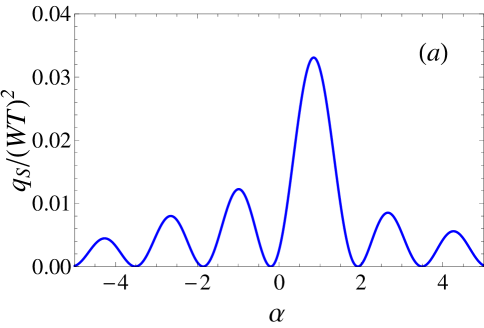
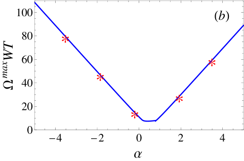
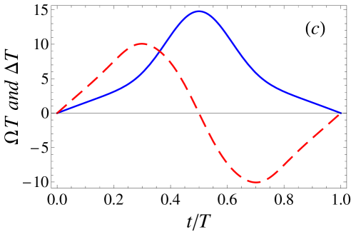
Figure 1: (Color online) (a) Systematic error sensitivity $q_{S}/(WT)^{2}$, Eq. (53), and (b) the Rabi frequency $\Omega^{\max}WT$, Eq. (55), versus $\alpha$, where the stars correspond to $\alpha$ with $q_{S}=0$. The coordinate of the start with the minimal $|\alpha|$ with $q_{S}=0$ is $(-0.206,14.784)$. (c) Rabi frequency $\Omega T$ (solid blue) and detuning $\Delta T$ (dotted red) versus time $t/T$, from Eqs. (37), (49), (50) and (51) with $W=1$, $\alpha=-0.206$.

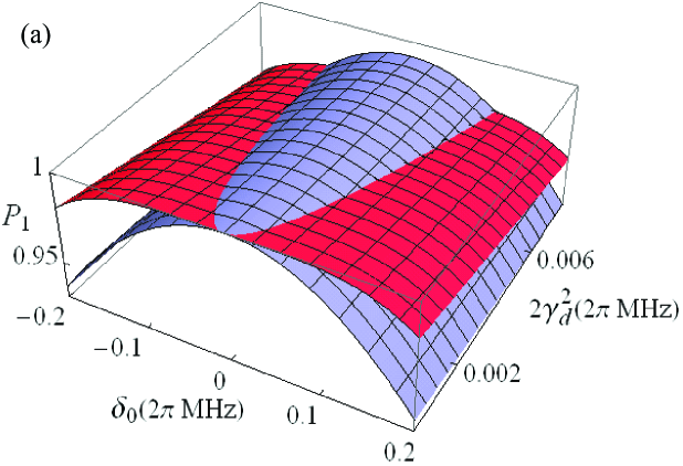
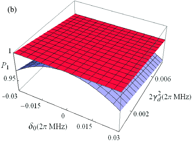
Figure 2: (Color online) Comparison of inversion probability $P_{1}(T)$ for two protocols. In (a) they share the same maximal Rabi frequency $\Omega^{\max}=0.784$ $\times$ 2$\pi$ MHz: one is a flat $\pi$-pulse, optimal for dephasing noise (light blue surface, prominent around $\delta_{0}=0$), with $T_{\pi}=\pi/\Omega^{\max}=0.638$ $\mu$s; the other one (dark red surface, more prominent around $\gamma_{d}=0$) has been optimized with respect to systematic frequency errors within the family described by Eqs. (37) and (49) with $T=3$ $\mu$s, $\alpha=-0.206$, and $W=1$. In (b) this later pulse remains the same but the $\pi$ pulse spans also $3$ $\mu$s, so that its $\Omega^{\max}=0.167\times 2\pi$ MHz.

VI Combined perturbations

Finally, we will consider both types of perturbations (noise and systematic error) together, so that $P_{1}(T)\approx 1-\gamma_{d}^{2}q_{N}-\delta_{0}^{2}q_{S}$. The best protocol in this case depends on the relative importance between dephasing noise and systematic error. Fig. 2 (a) depicts the final population $P_{1}(T)$ versus dephasing noise and systematic error perturbative parameters for two protocols that share the same $\Omega^{\max}$. The first one is a flat $\pi$ pulse (light blue surface), which is optimal with respect to dephasing noise ($q_{N}=T_{\pi}/2$, $q_{S}=(T_{\pi}/\pi)^{2}$, $\Omega=\Omega^{\max}=\pi/T_{\pi}$), and the second one (dark red surface) is described in the previous section ($\alpha=-0.206$, $q_{N}=[1+J_{0}(\pi)]TW/2$, $q_{S}=0$, $\Omega^{\max}=14.784/WT$. We choose $W=1$, $T=3$ $\mu$s, and $T_{\pi}=0.638$ $\mu$s so that $\Omega^{\max}$ takes the same value for both protocols. The $\pi$ pulse is the most stable when dephasing noise is dominant whereas the protocol that nullifies $q_{S}$ outperforms the $\pi$ pulse otherwise. In Fig. 2 (b) the $\pi$ pulse is modified to span also $T=3$ $\mu$s. This lowers its $\Omega^{\max}$ as well as its robustness.

VII Discussion

The design of fast and robust protocols for coherent population or state control of a quantum system depends strongly on the type of noise and/or perturbation. In a previous publication we designed, for the population inversion of a two-level atom in an electric field, driving fields which are robust with respect to amplitude noise or/and systematic perturbations of the Rabi frequency Andreas . Here we have considered instead excitation frequency shifts with constant offset and/or a white noise component that generates dephasing. When the Rabi frequency is not allowed to increase beyond a certain value, a flat $\pi$-pulse is the most robust approach versus phase noise but not with respect to systematic frequency shifts. The effect of systematic frequency shifts can be minimized (achieving zero sensitivity) with an alternative family of protocols. The results obtained here and in Andreas indicate that the standard claim that “adiabatic methods are robust whereas resonant $\pi$ pulses are not” does not apply to all possible perturbations. In other words, “robustness” is a relative concept. A protocol may be robust with respect to a particular perturbation but not to others. Depending on the physical conditions, it may be possible to nullify the sensitivity with respect to different perturbations simultaneously Andreas2013 . In the case of phase noise and frequency errors, only the sensitivity with respect to systematic frequency shifts can be nullified with finite energy.

The present techniques may as well be applied to find robust protocols for other perturbations and decoherence effects including spontaneous decay and bit-flip Sarandy07 , with applications in different quantum systems such as quantum dots spinQD , Bose-Einstein condensates in accelerated optical lattices Oliver , or quantum refrigerators Tova . Combining invariant-based engineering with optimal control techniques Gorman will allow for further stability with different physical constraints. This work may as well be generalized to consider colored phase noise and non-Markovian dephasing Yu ; Huelga ; Diosi1998 ; Yu-2 ; Guerin11 ; Vega , as well as alternative phase noise sources and master equations Poggi .

References

(1) L. Allen and J. H. Eberly, Optical Resonance and Two-level Atoms (Dover, New York, 1987).
(2) K. Bergmann, H. Theuer, and B. W. Shore, Rev. Mod. Phys. 70, 1003 (1998).
(3) N. V. Vitanov, T. Halfmann, B. W. Shore, and K. Bergmann, Annu. Rev. Phys. Chem. 52, 763 (2001).
(4) P. Král, I. Thanopulos, and M. Shapiro, Rev. Mod. Phys. 79, 53 (2007).
(5) M. Saffman, T. G. Walker, and K. Mølmer, Rev. Mod. Phys. 82, 2313 (2010).
(6) S. Guérin and H. R. Jauslin, Adv. Chem. Phys. 125, 147 (2003).
(7) A. Ruschhaupt, X. Chen, D. Alonso, and J. G. Muga, New J. Phys. 14, 093040 (2012).
(8) X. Chen, E. Torrontegui, and J. G. Muga, Phys. Rev. A 83, 062116 (2011).
(9) Y. Ban, X. Chen, E. Ya. Sherman and J. G. Muga, Phys. Rev. Lett., 109, 206602 (2012).
(10)H. R. Lewis and W. B. Riesenfeld, J. Math. Phys. 10, 1458 (1969).
(11) H.-P. Breuer and F. Petruccione, The Theory of Open Quantum Systems (Oxford University Press, Oxford, 2002).
(12) G. Lindblad, Commun. Math. Phys. 48, 119 (1976).
(13) M. S. Sarandy, E. I. Duzzioni, and M. H. Y. Moussa, Phys. Rev. A 76, 052112 (2007).
(14) E. S. Kyoseva and N. V. Vitanov, Phys. Rev. A 71, 054102 (2005).
(15) X. Lacour, S. Guérin, L. P. Yatsenko, N. V. Vitanov, and H. R. Jauslin, Phys. Rev. A 75, 033417 (2007).
(16) X. Lacour, S. Guérin, and H. R. Jauslin, Phys. Rev. A 78, 033417 (2008).
(17) P. M. Poggi, F. C. Lombardo, and D. A. Wisniacki, Phys. Rev. A 87, 022315 (2013).
(18) J.-F. Zhang, J. H. Shim, I. Niemeyer, T. Taniguchi, T. Teraji, H. Abe, S. Onoda, T. Yamamoto, T. Ohshima, J. Isoya, and D. Suter,
arXiv:1212.0832.
(19) D. Daems, A. Ruschhaupt, D. Sugny, and S. Guérin, arXiv:1304.4016 (2013).
(20) M. G. Bason, M. Viteau, N. Malossi, P. Huillery, E. Arimondo, D. Ciampini, R. Fazio, V. Giovannetti, R. Mannella, and O. Morsch, Nat. Phys. 8, 147 (2012).
(21)T. Feldman and R. Kosloff, EPL 89, 20004 (2010).
(22) D. J. Gorman, K. C. Young, and K. B. Whaley,
Phys. Rev. A 86, 012317 (2012).
(23) L. Diósi, N. Gisin, and W. T. Strunz, Phys. Rev. A 58, 1699 (1998).
(24) T. Yu, L. Diósi, N. Gisin, and W. T. Strunz, Phys. Rev. A 60, 91 (1999).
(25) I. deVega and D. Alonso, Phys. Rev. A 73, 022102 (2006).
(26) T. Yu and J. H. Eberly, Opt. Commun. 283, 676 (2010).
(27)S. Guérin, V. Hakobyan, and H. R Jauslin, Phys. Rev. A 84, 013423 (2011).
(28) S. F. Huelga, A. Rivas, and M. B. Plenio, Phys. Rev. Lett. 108, 160402 (2012).