Pairing of Zeros and Critical Points for Random Meromorphic Functions on Riemann Surfaces

Abstract.

We prove that zeros and critical points of a random polynomial $p_{N}$ of degree $N$ in one complex variable appear in pairs. More precisely, suppose $p_{N}$ is conditioned to have $p_{N}(\xi)=0$ for a fixed $\xi\in\mathbb{C}\backslash\{0\}.$ For $\epsilon\in\left(0,\frac{1}{2}\right)$ we prove that there is a unique critical point in the annulus $\left\{z\in\mathbb{C}\,\middle|\,N^{-1-\epsilon}<\left\lvert z-\xi\right\rvert<N^{-1+\epsilon}\right\}$ and no critical points closer to $\xi$ with probability at least $1-O(N^{-3/2+3\epsilon}).$ We also prove an analogous statement in the more general setting of random meromorphic functions on a closed Riemann surface.

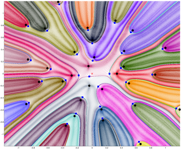
Figure 1. The zeros (black discs) and critical points (blue squares) of a degree $50$ $SU(2)$ polynomial $p_{50}$ appear in pairs. The typical distance between each pair is on the order of $\frac{1}{50}.$ Each pair lines up with the origin, denoted by a red asterisk. The gradient flow lines for $\log\left\lvert p_{50}\right\rvert^{2}$ are shown.

0. Introduction

The purpose of this article is to prove that zeros $\{z_{j}\}$ and critical points $\{c_{j}\}$ of random meromorphic functions on a Riemann surface come in pairs $(z_{j},c_{j})$ with $\left\lvert z_{j}-c_{j}\right\rvert\approx N^{-1},$ where $N$ is the common number of zeros and poles. To explain the result, consider $\mathcal{P}_{N}^{\xi},$ the space of polynomials in one complex variable of degree at most $N$ that vanish at a fixed $\xi\in\mathbb{C}=\mathbb{C}P^{1}\backslash\{\infty\}.$ We equip $P_{N}^{\xi}$ with a conditional gaussian measure $\gamma_{h,\xi}^{N}$ depending on a hermitian metric $h$ on $\mathcal{O}(1)\twoheadrightarrow\mathbb{C}P^{1}$ (see §0.2 for a precise definition). Consider the random variables

(0.1) $$\mathcal{N}_{r}:=\#\left\{z\in D_{r}(\xi)\,\middle|\,\frac{d}{dz}p_{N}(z)=0\right\},$$

where $D_{r}(\xi)$ is the disk of radius $r,$ and define $e^{-\phi_{z_{0}}(z)}:=\left\lVert z_{0}(z)\right\rVert_{h}^{2}$ for the usual frame $z_{0}$ of $\mathcal{O}(1)$ over $\mathbb{C}P^{1}\backslash\{\infty\}.$

Theorem 1.

Suppose $d\phi_{z_{0}}(\xi)\neq 0.$ For $\epsilon\in(0,\frac{1}{2}),$ write $R_{\pm}=N^{-1\pm\epsilon}.$ There is $K=K(\epsilon,h)$ so that

$$\gamma_{h,\xi}^{N}\left(\mathcal{N}_{R_{+}}=1\,\,\,\text{and}\,\,\,\mathcal{N}_{R_{-}}=0\right)\geq 1-K\cdot N^{-3/2+3\epsilon}.$$

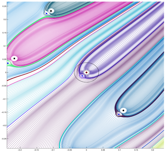
Figure 2. Zeros (black discs) and holomorphic critical points (blue squares) for an $SU(2)$ polynomial $p_{50}$ of degree $50$ conditioned to have a zero at $\xi=1+1i$ (denoted by a red asterisk) are drawn in normal coordinates centered at $\xi.$ The annulus with inner radius $N^{-1-1/10}$ and outer radius $N^{-1+1/10},$ which Theorem 1 perdicts to have a unique critical point is shown.

The pairing of zeros and critical points is illustrated in Figures 1 and 2. Typical nearest neighbor distance for $N$ i.i.d points on $\mathbb{C}P^{1}$ is $N^{-1/2}.$ We give a heuristic derivation of the much smaller $N^{-1}$ distance in Theorem 1 in terms of electrostatics on a Riemann surface in §2.2. In this paper, we focus on understanding the distance from a fixed zero to the nearest critical point for a random polynomial (or more generally meromorphic function on a Riemann surface). In §2.2 we also give a heuristic explanation for why paired zeros and critical points line up with the origin in Figure 1 and leave a rigorous characterization to future work (cf also Theorem 2 in [12]).

0.1. Riemann Surfaces

Zeros and critical points of random meromorphic functions on a closed Riemann surface $\Sigma$ also come in pairs. To study this situation we replace $\mathcal{P}_{N}^{\xi}$ with $H_{N}^{\xi},$ the space of sections of a very ample line bundle $L^{\otimes N}\twoheadrightarrow\Sigma$ that vanish at $\xi\in\Sigma.$ We generalize $\frac{d}{dz}$ by fixing an arbitrary section $\sigma_{N}\in H_{N}=H_{hol}^{0}(\Sigma,L^{N})$ and defining the meromorphic connection $\nabla^{\sigma_{N}}$ on $L^{N}$ via $\nabla^{\sigma_{N}}\sigma_{N}=0.$ The critical points of a section $s_{N}\in H_{N}^{\xi}$ are thus given by

(0.2) $$\nabla^{\sigma_{N}}s_{N}(z)=0.$$

The derivative $\frac{d}{dz}=\nabla^{z_{0}^{\otimes N}}$ on $\mathcal{O}(N)$ is of this form. For more on meromorphic connections see §5. Defining the meromorphic function $\gamma_{N}(z):=\frac{s_{N}(z)}{\sigma_{N}(z)}$ on $\Sigma,$ we see that

$$\nabla^{\sigma_{N}}s_{N}(z)=0\quad\longleftrightarrow\quad d\gamma_{N}(z)=0.$$

$d\gamma_{N}(z)=0$ is equivalent to $d\log\left\lvert\gamma_{N}(z)\right\rvert=0$ if $\gamma_{N}$ has simple zeros. We may therefore view $\left\lvert\gamma_{N}\right\rvert$ as a Coulomb potential on $\Sigma$ and interpret the critical point equation $d\log\left\lvert\gamma_{N}(z)\right\rvert=0$ as points of equilibrium for the electric field on $\Sigma$ generated by charge distributed according to the divisor of $\gamma_{N}.$ This perspective is developed in §2.2.

We emphasize that our notion of critical point is purlely holomorphic and results in a completely different theory from critical points computed with respect to smooth metric connections studied in [7, 8, 9, 10, 11]. We refer the reader to §2.4 for a discussion of this point.

0.2. Definition of Hermitian Guassian Ensembles

The ensembles of random sections we study are called Hermitian Gaussian Ensembles. They were first studied by Bleher, Shiffman and Zelditch in [2, 3, 15, 16]. Let $h$ be a smooth positive Hermitian metric on an ample holomorphic line bundle $L\twoheadrightarrow\Sigma$ over a closed Riemann surface. We recall the definition of the Hermitian Gaussian ensemble associated to $h.$ A random section of $L^{N}$ from this ensemble is

$$s_{N}:=\sum_{j=0}^{N}a_{j}S_{j},$$

where $a_{j}\sim N(0,1)_{\mathbb{C}}$ are i.i.d. standard complex Gaussians and $\{S_{j}\}_{j=0}^{N}$ is any orthonormal basis for $H_{N}$ with respect to the inner product

(0.3) $$\left\langle s_{1},s_{2}\right\rangle_{h}:=\int_{\Sigma}h^{N}(s_{1}(z),s_{2}(z))\,\omega_{h}(z),\quad s_{1},s_{2}\in H_{N}.$$

Here $\omega_{h}:=\frac{i}{2\pi}\partial\overline{\partial}\log h^{-2}$ is the curvature of $(L,h).$ We will write $\gamma_{h}^{N}$ for the law of $s_{N}$ and abbreviate $s_{N}\in HGE_{N}(L,h).$ In this paper, we focus on the following variant of $HGE_{N}(L,h):$

Definition 1.

For $\xi\in\Sigma$ fixed, we will write $s_{N}\in HGE_{N}^{\xi}(L,h)$ if the law of $s_{N}$ is the standard gaussian measure on

$$H_{N}^{\xi}=\left\{s_{N}\in H_{hol}^{0}(\Sigma,L^{N})\,\middle|\,s_{N}(\xi)=0\right\}$$

generated by the restriction of the inner product (0.3) to $H_{N}^{\xi}.$

We denote by $\gamma_{h,\xi}^{N}$ the law of $s_{N}\in HGE_{N}^{\xi}(L,h)$ and will write $s_{N}(z)=\sum_{j=1}^{d_{N}-1}a_{j}S_{j}^{\xi}(z),$ where $a_{j}$ are iid standard complex guassians and $\{S_{j}^{\xi},\,\,j=1,\ldots,d_{N}-1\}$ is any orthonormal basis for $H_{N}^{\xi}$ with respect to the inner product (0.3). Every $s_{N}\in HGE_{N}^{\xi}(L,h)$ satisfies $s_{N}(\xi)=0$ and may equivalently be defined as

$$s_{N}=\mathbb{E}\left[\widetilde{s}_{N}\,|\,ev_{\xi}(s_{N})=0\right],$$

where $\widetilde{s}_{N}\in HGE_{N}(L,h)$ and $ev_{\xi}:H_{hol}^{0}(\Sigma,L^{N})\rightarrow L^{N}|_{\xi}$ is the evaluation map at $\xi.$ See §3 of [18] for more details.

1. Main Result

Theorem 2 is our main result. We will need the following definition

Definition 2.

For $(L,h)\twoheadrightarrow\Sigma$ as above and $\sigma_{N}\in H_{hol}^{0}(L^{N}),$ define $\phi_{\sigma_{N}}:\Sigma\rightarrow(-\infty,\infty]$ by

$$\phi_{\sigma_{N}}:=\log\left\lVert\sigma_{N}\right\rVert_{h^{N}}.$$

Let $(L,h)\twoheadrightarrow\Sigma$ be as above and fix $\Gamma\in[0,\frac{1}{2})$ as well as $\sigma_{N}\in H_{hol}^{0}(L^{N})$ and $\xi\in\Sigma\backslash\{\sigma_{N}=0\}$ satisfying

(1.1) $$\left\lvert d\phi_{\sigma^{N}}(\xi)\right\rvert>C\cdot N^{1-\Gamma}$$

for some $C>0$ and all $N$ (cf §2.3 for the electorstatic interpretation of (1.1)).

Theorem 2.

Suppose $s_{N}\in HGE_{N}^{\xi}(L,h).$ For each $\epsilon\in(0,\frac{1}{2}-\Gamma)$ define $R_{\pm}=N^{-1+\Gamma\pm\epsilon}.$ Then there exists a constant $K=K(\Sigma,L,h,\Gamma,\epsilon),$ such that for each $N\geq 1$

(1.2) $$\gamma_{h,\xi}^{N}\left(\mathcal{N}_{R_{-}}=0\quad\text{and}\quad\mathcal{N}_{R_{+}}=1\right)\geq 1-K\cdot N^{-3/2+2\Gamma+3\epsilon}.$$

In the definition of $\mathcal{N}_{r},$ the disk $D_{r}$ is computed in Kähler normal coordinates centered at $\xi.$

Remark 1.

Let $\mu$ be any probability measure on $\prod_{N=1}^{\infty}H_{N}^{\xi}$ with marginals $\mu_{h,\xi}^{N}.$ Write $A_{N,\epsilon}$ for the event $\left\{\mathcal{N}_{R_{+}}=1\,\,\,\text{and}\,\,\,\mathcal{N}_{R_{-}}=0\right\}.$ If $2\Gamma+3\epsilon<\frac{1}{2},$ then we may apply the Borel-Cantelli Lemma to see that the events $A_{N,\epsilon}$ occur for all large enough $N$ $\mu-$almost surely.

2. Discussion

To explain the pairing of zeros and critical points, let us consider a degree $N$ random polynomial drawn from the $SU(2)$ ensemble studied in [12, 17, 18, 20, 21, 22]:

$$p_{N}(z):=\sum_{j=0}^{N}a_{j}\sqrt{\binom{N}{j}}\,z^{j}.$$

Here $a_{j}$ are iid standard complex gaussian random variables. The law of $p_{N}$ is $\gamma_{h_{FS}}^{N},$ where $h_{FS}$ is the Fubini-Study metric on $\mathcal{O}(1)\twoheadrightarrow\mathbb{C}P^{1}.$ $\gamma_{h_{FS}}^{N}$ is the unique centered gaussian on $\mathcal{P}_{N}$ for which the expected empirical measure of zeros is uniform on $\mathbb{C}P^{1}$ (cf §1.2 in [19]). The zeros and critical points of $p_{50}$ are drawn in Figure 1. The colored lines are gradient flow lines for the random morse function $G_{50}(z)=\log\left\lvert p_{50}(z)\right\rvert,$ whose local minima and saddle points are the zeros and critical points of $p_{50},$ respectively. There are no local maxima since $G_{50}$ is subharmonic. Flow lines of the same color terminate in the same zero or critical point.

2.1. Electrostatic Explanation for Pairing of Zeros and Critical Points

We now explain why most zeros $z_{j}$ are paired with unique nearby critical points $c_{j}$. We also explain why $\arg z_{j}\approx\arg c_{j}$ and $0<\left\lvert z_{j}\right\rvert-\left\lvert c_{j}\right\rvert\ll 1.$ In fact Theorem 1 shows that $\left\lvert z_{j}\right\rvert-\left\lvert c_{j}\right\rvert\approx N^{-1}.$

Let us distribute $N$ positive and $N$ negative charges on $\mathbb{C}P^{1}$ according to the divisor of $p_{N}.$ That is, we place $N$ positive delta charges at infinity and a single negative delta charge at each zero of $p_{N}.$ Write $E_{p_{N}}(z)\in T_{z}^{*}\mathbb{C}P^{1}$ for the resulting electric field at $z.$ As explained in §2.2, the critical point equation $\frac{d}{dz}p_{N}(z)=0,$ is equivalent to $E_{p_{N}}(z)=0.$

Suppose that $p_{N}(\xi)=0$ for some $\xi\neq 0.$ The remaining zeros of $p_{N}$ tend to be uniformly distributed on $\mathbb{C}P^{1}.$ For $z$ very near $\xi,$ the contribution to $E_{p_{N}}(z)$ from the remaining zeros is, heuristically, on the order of $N^{1/2}$ by the central limit theorem. To leading order in $N,$ $E_{p_{N}}(z)$ is thus the deterministic order of $N$ contribution from the $N$ positive delta charges at infinity and the single negative delta charge at $\xi.$

The Coulomb force in $1$ complex dimension at distance $r$ decays like $r^{-1}.$ Hence, for a configuration of $N$ positive charges at infinity and one negative charge at $\xi,$ a point of equilibrium for the electric field exists at a point $z$ a distance of order $N^{-1}$ away from $\xi$ in the direction of the line from infinity to $\xi.$ This is the electrostatic explanation for the pairing of zeros and critical points shown in Figures 1 and 2.

The pairing of zeros and critical points breaks down near the origin (the south pole) in Figure 1 because the electric field from the $N$ positive charges at infinity vanishes at the south pole. Critical points near $\xi=0$ are therefore determined by the locations of zeros with small modulus.

2.2. Electrostatics on Riemann Surfaces

We describe a theory of electrostatics on a closed Riemann surface $\Sigma$ that depends only on its complex structure. We will see that solutions to the critical point equation $d\gamma=0$ for a meromorphic function $\gamma:\Sigma\rightarrow\mathbb{C}P^{1}$ are precisely points of equilibrium for the electric field on $\Sigma$ from charges distributed according to its divisor

$$D:=\operatorname{Div}(\gamma)=\sum_{\gamma(z)=0}m(z)\delta_{z}-\sum_{\gamma(w)=\infty}m(w)\delta_{w}.$$

Here $m(\cdot)$ denotes the order of the relevant zero or pole of $\gamma.$ To begin, observe that $d\gamma=0$ is equivalent to $d\log\left\lvert\gamma\right\rvert=0$ as long as $\gamma$ has simple zeros. Let $\Delta=\frac{i}{\pi}\partial\overline{\partial}$ be the Laplacian mapping $\Omega^{0}(\Sigma)$ to $\Omega^{1,1}(\Sigma).$ By the Poincaré-Lelong formula, $G(z,D):=\log\left\lvert\gamma(z)\right\rvert,$ solves

(2.1) $$\Delta G(z,D)=D.$$

This is the analog of Poisson's Equation, which says that the Laplacian of the Coulomb potential gives the charge density.

Definition 3.

The electric co-field at $z$ from charge distribution $D$ is

$$E_{\gamma}(z):=dG(z,D_{\gamma})\in T_{z}^{*}\Sigma.$$

Since $\Sigma$ is compact, the equation $\Delta G=f$ has a solution only if $\int_{\Sigma}f=0.$ The price we pay for using only the complex structure of $\Sigma$ to define $E_{\gamma}$ is that we may work only with electrically netural charge distributions. As noted before, the critical point equation $d\gamma(z)=0$ is generically equivalent to $d\log\left\lvert\gamma(z)\right\rvert=0$ and hence to $E_{\gamma}(z)=0.$

2.3. Meaning of $\phi_{\sigma_{N}}$

The quantity $d\phi_{\sigma_{N}}$ (Definition 2) plays a key role in our results. To see why, note that

$$\frac{i}{2\pi}\partial\overline{\partial}\log\left\lVert\sigma_{N}(z)\right\rVert_{h}^{-2}=N\omega_{h}-Z_{\sigma_{N}}.$$

As in §0.2, $\omega_{h}$ is the curvature form of $h$ and $Z_{\sigma_{N}}$ is the current of integration over the zero set of $\sigma_{N}.$ The term $N\omega_{h}$ is essentially $\mathbb{E}\left[Z_{s_{N}}-\delta_{\xi}\right]$ for $s_{N}\in HGE_{N}^{\xi}(L,h)$ (cf e.g. Theorem 1 in [18], Lemma 3.1 in [15], and Lemma 2 in §5 of [12]). Let us write as in §2.1 $E_{\frac{s_{N}}{\sigma_{N}}}(\xi)$ for the electric field at $\xi$ from charge distributed according to $Z_{s_{N}}-\delta_{\xi}-Z_{\sigma_{N}}.$ Then

$$d\phi_{\sigma_{N}}(\xi)\approx\mathbb{E}\left[E_{N}(\xi)\right].$$

The contribution of the random zeros of $s_{N}$ should heuristically be on the order of $N^{1/2}$ by the central limit theorem. The condition that $\left\lvert d\phi_{\sigma_{N}}(\xi)\right\rvert>N^{1-\Gamma}$ for some $\Gamma<\frac{1}{2}$ is equivalent to asking that the average electric field at $\xi$ be dominated by the deterministic contribution from the charges at $\xi$ and at $Z_{\sigma_{N}}.$ Points $z\in\Sigma$ for which $d\phi_{\sigma_{N}}(z)=0,$ for example, play the same role as the origin for the $SU(2)$ ensemble (cf the end of §2.1).

2.4. Smooth Versus Holomorphic Critical Points

The critical points we study solve the equation

(2.2) $$\nabla^{\sigma_{N}}s_{N}(z)=0\quad\longleftrightarrow\quad\frac{d}{dz}\left(\frac{s_{N}(z)}{\sigma_{N}(z)}\right)=0.$$

Smooth critical points (cf e.g. [7, 8, 9]), in contrast, are solutions of

(2.3) $$\nabla^{h}s_{N}(z)=0\quad\longleftrightarrow\quad\frac{d}{dz}\left\lVert s_{N}(z)\right\rVert_{h}=0,$$

where $\nabla^{h}$ is the Chern connection of $h.$ The two settings are qualitatively different. For instance, the zeros of $s_{N}\in HGE_{N}(L,h)$ repel (cf e.g. the Introductions in [3] and[18]). Hence, since zeros and holomorphic critical points tend to apear in pairs, solutions to (2.2) repel as well. This can be seen directly by computing the two point function for holomorphic critical points, although we do not do this in the present paper. In contrast, Baber in [1] showed that smooth critical points of $s_{N}$ actually attract. Further, the number of holomorphic critical points depends only on $L,$ $N$, and $\sigma_{N}$ by the Riemann-Roch formula. The number of smooth critical points is, on the other hand, a non-degenerate random variable, whose expected value is $\frac{5N}{3}$ to leading order in $N$ (cf Corollary 5 and §6 in [7]).

Smooth critical points were implicitly studied in the work of Nazarov, Sodin, and Volberg [14], where a so-called ``gravitational allocation'' was constructed between the counting measure for zeros of a gaussian analytic function $f(z)$ and Lebesgue measure on $\mathbb{C}.$ The allocation is achieved by gradient flow for the potential $\left\lVert f(z)\right\rVert_{h}^{2},$ where $h(z)=\frac{1}{\pi}e^{-\left\lvert z\right\rvert^{2}}$ is the usual hermitian metric on $\mathbb{C}\times\mathbb{C}\twoheadrightarrow\mathbb{C}.$ The saddle points for this potential are critical points of $f$ with respect to the Chern connection of $h.$ The analogous gravitational allocation in Figures 1 and 2 uses $\left\lvert p_{N}(z)\right\rvert^{2}$ as a potential, omitting the smooth metric factor. Finally, we mention that the expected distribution of critical values for smooth critical points was worked out in [10] and [11].

3. Acknowledgements

I am grateful to S. Zelditch for many helpful conversations about his work previous work on statistics of zeros and critical points and for his comments on an earlier draft of this paper. I would also like to thank R. Peled for sharing with me M. Krishnapur's code that I modified to generate the figures in this paper.

4. Outline

The remainder of this paper is organized as follows. First, in §5, we give some background on meromorphic connections. Then, in §6, we establish notation to be used throughout. In §7 we recall relevant facts about Bergman kernels. Namely, in §7.1-7.2 we recall their definition and in §7.3-7.4 we recall their asymptotic expansions as given by Zelditch and Shiffman in [16]. Finally, in the appendix, §9, we derive asymptotics for derivatives of the Bergman kernel. These asymptotics will be the key analytic formulas underlying the proof of Theorem 2, which is given in §8.

5. Meromorphic Connections on $L\twoheadrightarrow\Sigma$

Definition 4.

A meromorphic connection on $L\twoheadrightarrow\Sigma$ is a connection $\nabla$ on $L$ with the following mapping property:

$$\nabla:H_{mer}^{0}(\Sigma)\rightarrow H_{mer}^{0}(\Sigma)\otimes_{\mathcal{O}_{mer}(\Sigma)}\Omega^{1,0}(\Sigma).$$

We study critical points of random sections of $L$ and its tensor powers with respect to a special class of meromorphic connections. For $\sigma\in H_{hol}^{0}(\Sigma,L)$ the equation $\nabla^{\sigma}\sigma=0$ defines the meromorphic connection $\nabla^{\sigma}$ up a constant multiple. For $s\in H_{hol}^{0}(L)$

$$\nabla^{\sigma}s=\nabla^{\sigma}\frac{s}{\sigma}\sigma=d\left(\frac{s}{\sigma}\right)\cdot\sigma\in H_{mer}^{0}(L)\otimes\Omega^{1}(\Sigma).$$

This formula shows that $\nabla^{\sigma}$ introduces a pole at each zero of $\sigma$ (not counting multiplicity).

Meromorphic connections $L$ are natural generalizations of the holomorphic derivative $\frac{d}{dz}.$ Indeed, if we write $z_{0}$ for the usual frame for $\mathcal{O}(1)\twoheadrightarrow\mathbb{C}P^{1}\backslash\{[0:1]\}.$ The section $z_{0}^{N}$ induces the trivialization

$$\alpha_{N}:\mathcal{O}(N)\big{|}_{\mathbb{C}P^{1}\backslash{\{\infty\}}}\stackrel{{\scriptstyle\cong}}{{\longrightarrow}}\mathbb{C}\times\mathbb{C},$$

which identifies $H_{hol}^{0}(\mathbb{C}P^{1},\mathcal{O}(N))$ with $\mathcal{P}_{N},$ the polynomials of degree up to $N.$ We may define then define a meromorphic connection $\nabla^{z_{0}^{N}}:=\alpha_{N}^{*}d$ on $\mathcal{O}(N).$ We note that the section $z_{0}^{N}$ corresponds to the constant polynomial $1$ and hence is parallel for $\nabla^{z_{0}^{N}},$ in agreement with our earlier notation. Moreover, $z_{0}$ vanishes only at $[0:1]$ and hence $\nabla^{z_{0}^{N}}$ has a simple pole at $[0:1].$ See §3 in [12] for more details.

6. Notation

In §0.2, we wrote $s_{N}=\sum_{j=1}^{d_{N}}a_{j}S_{j}\in HGE_{N}(L,h).$ Consider $\Phi_{N}:\Sigma\rightarrow\mathbb{C}P^{d_{N}-1}$ defined by

$$\Phi_{N}(z)=[S_{1}(z):\cdots:S_{d_{N}}(z)].$$

We will refer to $\Phi_{N}$ as the coherent states embedding generated by $h.$ Since $L$ is ample, the space $H_{hol}^{0}(\Sigma,L^{N})$ is basepoint free for $N$ large and hence $\Phi_{N}$ is well-defined. The map $\Phi_{N}$ is an almost-isometry (cf [23]):

$$\left\lVert\omega_{h}-\frac{1}{N}\Phi_{N}^{*}\omega_{FS}\right\rVert_{C^{\infty}}=O(N^{-1}).$$

Here $\omega_{h}$ is the curvature form of $h$ and $\omega_{FS}$ is the Fubini-Study metric on $\mathbb{C}P^{d_{N}}.$ This result is Corollary $3$ in [24] and was proved independently by Catlin in [5]. We will write

$$s_{N}=\left\langle a,\Phi_{N}\right\rangle$$

for $a=(a_{1},\ldots,a_{d_{N}})$ a standard complex gaussian vector on $H_{hol}^{0}(\Sigma,L^{N}).$ We assume fixed throughout a distinguished section $\sigma_{N}\in H_{hol}^{0}(\Sigma,L^{N}),$ which is parallel for the meromorphic connection $\nabla^{\sigma_{N}}$ with respect to which we compute critical points. We will write

$$S_{j}=f_{j}\cdot\sigma_{N}$$

whenever we do local computations. Theorem 2 concerns sections $s_{N}(z)=\sum_{j=1}^{d_{N}-1}a_{j}S_{j}^{\xi}(z)\in HGE_{N}^{\xi}(L,h),$ where, as before, $\{S_{j}^{\xi}\}$ is an orthonomal basis for $H_{N}^{\xi}$ (defined in the Introduction) with respect to the inner product (0.3). As in the unconditional ensemble, we will write

$$s_{N}(z)=\left\langle a,\Phi_{N}^{\xi}(z)\right\rangle,$$

where $\Phi_{N}^{\xi}:\Sigma\rightarrow\mathbb{C}P^{d_{N}-2}$ is given in homogeneous coordinates by $\Phi_{N}^{\xi}(z)=[S_{1}^{\xi}(z):\cdots:S_{d_{N}-1}^{\xi}(z)]$ and set $S_{N}^{\xi}=f_{j}^{\xi}\cdot\sigma_{N}.$ Abusing notation, $\Phi_{N}^{\xi}$ will sometimes denote a map $\Phi_{N}^{\xi}:\Sigma\rightarrow\mathbb{C}^{d_{N}-1}$ given by $\Phi_{N}^{\xi}(z)=\left(f_{1}^{\xi}(z),\ldots,f_{d_{N}-1}^{\xi}(z)\right).$ We will refer to $\Phi_{N}^{\xi}$ as the conditional coherent states embedding generated by $h$ relative to the frame $\sigma_{N}.$

7. Bergman and Szegö Kernels

Let us recall some background on Bergman kernels. In §7.1, we define the $N^{th}$ Bergman kernel $\Pi_{N}$ of $(L,h).$ The related conditional Bergman kernel $\Pi_{N}^{\xi}$ is the covariance kernel of the Gaussian field $s_{N}\in HGE_{N}^{\xi}(L,h).$ In §7.2, we introduce the conditional normalized Bergman kernel $P_{N}^{\xi},$ key in the proof of Theorem 2. Our main technical tool is the $C^{\infty}$ asymptotic expansion for $\Pi_{N}$ derived by Shiffman and Zelditch in [16, 17], which we recall in §7.4. Off-diagonal Bergman kernel asymptotic expansions are given also in [13] and in [6]. To explain this asymptotic expansion we recall in §7.3 the principal $S^{1}$ bundle $X\twoheadrightarrow\Sigma$ associated to $(L,h)\twoheadrightarrow\Sigma.$ The family of kernels $\Pi_{N}$ are analyzed by lifting to $X,$ where they are naturally interpreted as Szëgo kernels. In the appendix, §9, we derive asymptotic expansions for derivatives of $\Pi_{N}^{\xi}$ with respect to the meromorphic connection $\nabla^{\sigma_{N}}.$

7.1. Definition of $\Pi_{N}$ and $\Pi_{\sigma_{N}}$

We make the following

Definition 5.

The covariance kernel for $s_{N}=\sum_{j=1}^{d_{N}}a_{j}S_{j}\in HGE_{N}(L,h)$ is called the $N^{th}$ Bergman kernel for $(L,h):$

(7.1) $$\Pi_{N}(z,w):=\operatorname{Cov}(p_{N}(z),p_{N}(w))=\sum_{j=0}^{N}S_{N}^{j}(z)\otimes\overline{S_{N}^{j}(w)}\in H_{hol}^{0}(\Sigma,L^{N}\otimes\overline{L^{N}}).$$

The family of Bergman kernels $\Pi_{N}$ is well-understood for a positive holomorphic line bundle $(L,h)\twoheadrightarrow M$ over a compact Kähler manifold $M$ (cf [16, 17]). If we fix a local frame $e$ for $L^{N}$ and write $S_{j}=\gamma_{j}\cdot e,$ then we can make the following

Definition 6.

The $N^{th}$ Bergman kernel for $(L,h)$ relative to the frame $e$ is

$$\Pi_{e}(z,w):=\sum_{j=1}^{d_{N}}\gamma_{j}(z)\overline{\gamma_{j}(w)}.$$

We observe that $\Pi_{e}(z,w)\cdot e(z)\otimes\overline{e(w)}=\Pi_{N}(z,w).$ Writing $s_{N}(z)=\sum_{j=0}^{d_{N}-1}a_{j}S_{j}^{\xi}(z)\in HGE_{N}^{\xi}(L,h),$ we define the $N^{th}$ conditional Bergman kernel to be

$$\Pi_{N}^{\xi}(z,w):=\sum_{j=1}^{d_{N}-1}S_{j}^{\xi}(z)\otimes\overline{S_{j}^{\xi}(w)}.$$

Similarly, writing $S_{j}^{\xi}=\gamma_{j}^{\xi}\cdot e$ for any frame $e$ of $L^{N},$ we define the $N^{th}$ conditional Bergman kernel relative to the frame $e$ to be

$$\Pi_{e}^{\xi}:=\sum_{j=1}^{d_{N}-1}\gamma_{j}^{\xi}(z)\overline{\gamma_{j}^{\xi}(w)}$$

and note that

(7.2) $$\Pi_{N}^{\xi}(z,w)=\Pi_{e}^{\xi}(z,w)\cdot e(z)\otimes\overline{e(w)}.$$

7.2. Normalized Bergman Kernel

The local statistics of the critical points for $s_{N}\in HGE_{N}^{\xi}(L,h)$ are conveniently expressed in terms of the normalized Bergman kernel for the conditional ensemble $HGE_{N}^{\xi}(L,h)$ (cf [12, 17, 18]):

(7.3) $$P_{N}^{\xi}(z,w):=\frac{\left\lVert\nabla^{\sigma_{N}}\otimes\overline{\nabla^{\sigma_{N}}}\Pi_{N}^{\xi}(z,w)\right\rVert_{h^{N}}}{\sqrt{\left\lVert\nabla^{\sigma_{N}}\otimes\overline{\nabla^{\sigma_{N}}}\Pi_{N}^{\xi}(z,z)\right\rVert_{h^{N}}\left\lVert\nabla^{\sigma_{N}}\otimes\overline{\nabla^{\sigma_{N}}}\Pi_{N}^{\xi}(w,w)\right\rVert_{h^{N}}}}.$$

The analysis of $P_{N}^{\xi}$ will play a crucial role in the proof of Theorem 2. Probabilitistically, $P_{N}^{\xi}(z,w)$ is the correlation between the random variables $\nabla^{\sigma_{N}}s_{N}(z)$ and $\nabla^{\sigma_{N}}s_{N}(w)$ for $s_{N}\in HGE_{N}^{\xi}(L,h).$

7.3. Principal $S^{1}$ Bundle

Consider a positive line bundle $(L,h)\twoheadrightarrow M$ over a compact Käher manifold and an orthonormal basis $\{S_{j}\}_{j=0}^{d_{N}}$ for $H_{hol}^{0}(L^{N})$ with respect to the inner product (0.3). The $N^{th}$ Bergman kernel $\Pi_{N}(z,w)=\sum_{j=0}^{d_{N}}S_{j}(z)\otimes\overline{S_{j}(w)}$ is studied in [16] by lifting sections $s\in H_{hol}^{0}(L^{\otimes N})$ to $S^{1}$-equivariant functions on the principal $S^{1}$ bundle associated to $(L,h),$ where the parametrix construction of Botet de Monvel and Sjöstrand in [4] may be applied. More precisely, we write $h^{*}$ for the dual metric on the dual bundle $L^{*}$ and define the principle $S^{1}$ bundle $X\twoheadrightarrow M$ by

$$X:=\left\{v\in L^{*}\,\middle|\,\left\lVert v\right\rVert_{h^{*}}=1\right\}.$$

We denote by $\widehat{s}$ the lift of a section $s$ to the function $\widehat{s}(v):=v^{\otimes N}(s)$ on $X.$ Writing $s=f\cdot e^{\otimes N}$ for a local frame $e$ of $L,$ and using $e^{*}$ to trivialize $X,$ we may write

(7.4) $$\widehat{s}(\theta,z):=e^{iN\theta}\left\lVert e(z)\right\rVert_{h}^{N}\cdot f(z).$$

Observe that

(7.5) $$\left\lvert\widehat{s}(\theta,z)\right\rvert=\left\lVert s(z)\right\rVert_{h^{N}}.$$

The lifted Bergman kernel is then

$$\widehat{\Pi}_{N}(\alpha,z;\beta,w):=\sum_{j=0}^{N}\widehat{S_{j}}(\alpha,z)\overline{\widehat{S_{j}}(\beta,w)}.$$

We observe that $\widehat{\Pi}_{N}$ is the Szegö kernel for the Hardy space of $X.$ See §1.2 of [16] for further details. In this paper, we are interested in the special case $M=\Sigma,$ a closed Riemann surface. The following two definitions from §2.2 of [17] allow us to formulate the $C^{\infty}$ complete asymptotic expansion for $\widehat{\Pi}_{N}$ derived there.

Definition 7.

Fix $\xi\in\Sigma$ and $e$ a frame for $L$ in a neighborhood $U$ containing $\xi.$ The frame $e$ is called a preffered frame for $h$ at $\xi$ if in a Kähler normal coordinate $z:U\rightarrow\mathbb{C}$ centered at $\xi,$ we have

$$\left\lVert e(z)\right\rVert_{h}=1-\frac{1}{2}\left\lvert z\right\rvert^{2}+o(\left\lvert z\right\rvert^{2}).$$

Definition 8.

Fix $\xi\in\Sigma,$ a Kähler normal coordinate $\psi:U\rightarrow\mathbb{C}$ centered at $\xi,$ and a preferred frame $e$ for $h$ at $\xi.$ Denoting by $\pi$ the projection map $\pi:X\twoheadrightarrow M,$ a Heisenberg coordinate on $X$ centered at $\xi$ is a coordinate $\rho:S^{1}\times\mathbb{C}\rightarrow\pi^{-1}(U)$ given by

(7.6) $$\rho(\theta,\psi(z))=e^{i\theta}\left\lVert e(z)\right\rVert_{h}e^{*}(z).$$

A Heisenberg coordinate on $X$ is therefore the choice of a Kähler normal coordinate on $\Sigma$ centered at $\xi$ and a trivialization of $X$ by a preferred frame at $\xi.$ The role of Heisenberg coordinates is that in these special local coordinates, the Szegö kernels $\widehat{\Pi}_{N}$ have a universal scaling limit depending only on $\dim_{\mathbb{C}}M.$ We refer the interested reader to §1.3.2 of [3] for more details.

7.4. Asymptotic Expansion for $\Pi_{N}$

We now recall for the particular case of $L\twoheadrightarrow\Sigma$ the on-diagonal, near off-diagonal, and far off-diagonal asymptotics for the Szegö kernels $\Pi_{N}$ derived in [16] and [17] by Shiffman and Zelditch. We note that the on-diagonal asymptotics were obtained also by Catlin in [5] off-diagonal expansions appeared in [6, 13]. The following is a special case of Theorem 2.4 from [17].

Theorem 3.

Fix Heisenberg coordinates on $X$ around $\xi\in\Sigma.$ Suppose $b>\sqrt{j+2k},~{}j,k\geq 0:$
1. Far Off-Diagonal. For $d(z,w)>b\left(\frac{\log N}{N}\right)^{1/2}$ and $j\geq 0,$ we have

(7.7) $$\nabla^{j}\widehat{\Pi}_{N}(\alpha,z;\beta,w)=O(N^{-k}),$$

where $\nabla^{j}$ denotes the horizontal lift to $X$ of any $j$ mixed derivatives in $z,\overline{z},w,\overline{w}.$
2. Near Off-Diagonal. Let $\epsilon>0.$ In Heisenberg coordinates (see Definition 8) centered at $\xi,$ we have for $\left\lvert z\right\rvert+\left\lvert w\right\rvert<b\left(\frac{\log N}{N}\right)^{1/2}$

(7.8) $$\widehat{\Pi}_{N}\left(\alpha,z;\beta,w\right)=e^{iN(\alpha-\beta)-z\cdot\overline{w}+\frac{1}{2}\left(\left\lvert z\right\rvert^{2}+\left\lvert w\right\rvert^{2}\right)}[1+R_{N}(z,w)],$$

where

(7.9) $$\nabla^{j}R_{N}(z,w)=O(N^{-1/2+\epsilon}),$$

and the implied constant in equation (7.9) is allowed to depend on $\epsilon.$ The remainder $R_{N}$ satisfies in addition, for $j=0,1,2$

(7.10) $$\left\lvert\nabla^{j}R_{N}(z,w)\right\rvert=O(\left\lvert z-w\right\rvert^{2-j}N^{-1/2+\epsilon})$$

uniformly for $\left\lvert z\right\rvert+\left\lvert w\right\rvert<\left(\frac{\log N}{N}\right)^{1/2}$ with the implied constants are independent of $N.$

8. Proof of Theorem 2

We first recall the notation. Let $\sigma_{N}\in H_{hol}^{0}(\Sigma,L^{N})$ be fixed, and define

$$\phi_{N}(z)=\log\left\lVert\sigma_{N}\right\rVert_{h}^{-2}.$$

Consider $\xi\in\Sigma\backslash\{\sigma_{N}=0\}$ such that $\left\lvert d\phi_{N}(\xi)\right\rvert>C\cdot N^{1-\Gamma}$ for a fixed $\Gamma\in[0,1/2)$ and a universal constant $C.$ In a Kähler normal coordinate around $\xi,$ we wrote

$$\mathcal{N}_{r}:=\#\left\{w\in D_{r\cdot N^{-1/2}}(\xi)\,\middle|\,\nabla^{\sigma_{N}}s_{N}(w)=0\right\},$$

where $D_{R}(\xi)$ is the disk of radius $R$ in our fixed coordinate system. We fix an $\epsilon>0$ such that $\Gamma+\epsilon<1/2$ and abbreviate $R_{\pm}:=N^{-1/2+\Gamma\pm\epsilon}.$ The conclusion of Theorem 2 follows easily from Lemmas 1 and 2, which we prove in Sections 8.1 and 8.2, respectively.

Lemma 1.

Fix $\epsilon>0$ such $\Gamma+\epsilon<1/2.$ We have

(8.1) $$\mathbb{E}\left[\mathcal{N}_{R_{+}}\right]=1+O(N^{-\epsilon}).$$

Similarly,

(8.2) $$\mathbb{E}\left[\mathcal{N}_{R_{-}}\right]=O(N^{-\epsilon}).$$

The implied constants in $O(N^{-\epsilon})$ depend only on $\epsilon.$

Lemma 2.

For any $\epsilon>0$, if $r\leq N^{-1/2+\Gamma+\epsilon},$ then we have

$$\operatorname{Var}[\mathcal{N}_{r}]=O(N^{-3/2+2\Gamma+3\epsilon}).$$

The implied constant depends only on $\epsilon.$

Indeed, since $N_{r}$ is an integer valued random variance, by Chebyshev's inequality:

$$P\left(\left(\mathcal{N}_{R_{+}}=1\cap\mathcal{N}_{R_{-}}=0\right)^{c}\right) \leq P\left(\mathcal{N}_{R_{+}}\neq 1\right)+P\left(\mathcal{N}_{R_{-}}\neq 0\right)$$

$$\leq P\left(\left\lvert\mathcal{N}_{R_{+}}-\mathbb{E}\left[\mathcal{N}_{R_{+}}\right]\right\rvert>1+O(N^{-\epsilon})\right)$$

$$\,\,+P\left(\left\lvert\mathcal{N}_{R_{-}}-\mathbb{E}\left[\mathcal{N}_{R_{-}}\right]\right\rvert>1+O(N^{-\epsilon})\right)$$

$$\leq\frac{\operatorname{Var}[\mathcal{N}_{R^{+}}]+\operatorname{Var}[\mathcal{N}_{R_{\epsilon}^{-}}]}{1+O(N^{-\epsilon})}$$

$$=O(N^{-3/2+2\Gamma+3\epsilon}).$$

8.1. Proof of Lemma 1

Since $\sigma_{N}(\xi)\neq 0,$ we may write as in §6 $s_{N}=p_{N}\cdot\sigma_{N}=\left\langle a,\Phi_{N}^{\xi}\right\rangle\cdot\sigma_{N},$ where $a=\left(a_{0},\ldots,a_{d_{N}}\right)$ is a standard gaussian vector on $H_{N}^{\xi}$ and $\Phi_{N}^{\xi}(z)=\left(f_{1}^{\xi}(z),\cdots,f_{d_{N}}^{\xi}(z)\right)$ is the coherent states embedding relative to the frame $\sigma_{N}.$ We will write

$$\frac{d}{dz}\Phi_{N}^{\xi}(z)=\left(\frac{d}{dz}f_{1}^{\xi}(z),\cdots,\frac{d}{dz}f_{d_{N}}^{\xi}(z)\right).$$

The $N^{th}$ conditional Bergman kernel relative to $\sigma_{N}$ (introduced in §7.1) is therefore $\Pi_{\sigma_{N}}^{\xi}(z,w)=\sum_{j=1}^{d_{n}}f_{j}^{\xi}(z)\overline{f_{j}^{\xi}(w)}.$ Our proof of Lemma 1 proceeds in two steps:

1. First, in Lemma 3, we write, for any $r>0,$ $\mathbb{E}\left[\mathcal{N}_{r}\right]$ in terms of $\Pi_{\sigma_{N}}^{\xi}(z,w)$ by using the Poincaré-Lelong formula:

   $$\mathbb{E}\left[\mathcal{N}_{r}\right]=\frac{r}{2\pi}\int_{0}^{2\pi}I(re^{i\theta})d\theta,$$

   where

   $$I(z):=\frac{d}{dz}\log\left(\frac{d^{2}}{dzd\overline{w}}\bigg{|}_{z=w=re^{i\theta}}\Pi_{\sigma_{N}}^{\xi}(\widehat{z},\widehat{w})\right)\cdot e^{i\theta},$$

   and $\widehat{u}=u\cdot N^{-1/2}.$

2. We then complete the proof by using the estimate (9.3) to see that if $\left\lvert z\right\rvert=R_{+},$ then $I(z)=\frac{R_{+}^{-1}\left(1+O(N^{-\epsilon})\right)}{1+O(N^{-\epsilon})},$ while if $\left\lvert z\right\rvert=R_{-},$ then $I(z)=\frac{O(R_{-}^{-1}N^{-\epsilon})}{1+O(N^{-\epsilon})}.$

Lemma 3.

We have

(8.3) $$\mathbb{E}\left[\mathcal{N}_{r}\right]=\frac{r}{2\pi}\int_{0}^{2\pi}\frac{d}{dz}\log\left(\frac{d^{2}}{dzd\overline{w}}\bigg{|}_{z=w=re^{i\theta}}\Pi_{\sigma_{N}}^{\xi}(\widehat{z},\widehat{w})\right)\cdot e^{i\theta}d\theta.$$

Proof.

The Poincaré-Lelong formula states the current of integration on the zero set of a non-zero analytic function $f$ is $Z_{f}=\frac{i}{2\pi}\partial\overline{\partial}\log\left\lvert f\right\rvert^{2}.$ Hence,

(8.4) $$\mathcal{N}_{r}=\int_{D_{r\cdot N^{-1/2}}}Z_{p_{N}}=\int_{D_{r\cdot N^{-1/2}}}\frac{i}{2\pi}\partial_{z}\overline{\partial}_{z}\log\left\lvert\frac{d}{dz}p_{N}(z)\right\rvert^{2}.$$

Since $\partial\overline{\partial}=-d\partial,$ we may use Stokes theorem to write

(8.5) $$\mathcal{N}_{r}=\frac{1}{2\pi i}\oint_{\partial D_{r\cdot N^{-1/2}}}\partial\log\left\lvert\frac{d}{dz}p_{N}(z)\right\rvert^{2}=\frac{1}{2\pi i}\oint_{\partial D_{r}}\partial\log\left\lvert p_{N}(\widehat{z})\right\rvert^{2}.$$

Applying Fubini's theorem and differentiating under the integral sign, we find that

$$\mathbb{E}\left[\mathcal{N}_{r}\right]=\frac{r}{2\pi}\int_{0}^{2\pi}\frac{d}{dz}\mathbb{E}\left[\log\left\lvert\frac{d}{dz}p_{N}(re^{i\theta}\cdot N^{-1/2})\right\rvert^{2}\right]\cdot e^{i\theta}d\theta.$$

Writing $\left\lVert\cdot\right\rVert$ for the $l_{2}$ norm a vector, we note that

$$\mathbb{E}\left[\log\left\lvert\frac{d}{dz}p_{N}(\widehat{z})\right\rvert\right]^{2}=\mathbb{E}\left[\log\left\lvert\left\langle a,\frac{\frac{d}{dz}\Phi_{N}^{\xi}(\widehat{z})}{\left\lVert\frac{d}{dz}\Phi_{N}^{\xi}(\widehat{z})\right\rVert}\right\rangle\right\rvert^{2}\right]+\log\left\lVert\frac{d}{dz}\Phi_{N}^{\xi}(\widehat{z})\right\rVert^{2}.$$

Since the gaussian measure is unitarily invariant, we see that the first term is $\mathbb{E}\left[\log\left\lvert a_{1}\right\rvert\right],$ and there is therefore annihilated by $\frac{d}{dz}.$ The following observation completes the proof:

$$\left\lVert\frac{d}{dz}\Phi_{N}^{\xi}(\widehat{z})\right\rVert^{2}=\sum_{j=1}^{d_{N}}\left\lvert\frac{d}{dz}f_{j}^{\xi}(\widehat{z})\right\rvert^{2}=\frac{d^{2}}{dzd\overline{w}}\bigg{|}_{z=w}\Pi_{\sigma_{N}}^{\xi}(\widehat{z},\widehat{w}).$$

∎

Combining formula (8.3) with (9.2), we find

(8.6) $$\mathbb{E}\left[\mathcal{N}_{r}\right]=\frac{r}{2\pi}\int_{0}^{2\pi}\left(N^{-1/2}\frac{\partial}{\partial z}\bigg{|}_{z=re^{i\theta}}\phi_{N}(\widehat{z})+\frac{d}{dz}\bigg{|}_{z=re^{i\theta}}\log T(z,z)+O(N^{-1/2+\epsilon})\right)e^{i\theta}d\theta.$$

We may taylor expand to write

$$\frac{\partial\phi_{N}}{\partial z}(\widehat{z})=\frac{\partial\phi_{N}}{\partial z}(\xi)+O(\left\lvert z\right\rvert N^{-1/2}).$$

Hence,

$$\frac{r}{2\pi}\int_{0}^{2\pi}N^{-1/2}\frac{\partial}{\partial z}\bigg{|}_{z=re^{i\theta}}\phi_{N}(\widehat{z})e^{i\theta}d\theta=O(r^{2}N^{-1}).$$

Therefore, we find

$$\mathbb{E}\left[\mathcal{N}_{r}\right]=\frac{r}{2\pi}\int_{0}^{2\pi}\frac{d}{dz}\bigg{|}_{z=re^{i\theta}}\log T(z,z)e^{i\theta}d\theta+O(rN^{-1/2+\epsilon}).$$

Finally, using the estimate (9.3), we have

$$\frac{d}{dz}\bigg{|}_{z=R_{-}\cdot e^{i\theta}}\log T(z,z)=\frac{R_{-}^{-1}\left(e^{-i\theta}+O(N^{-1/2+\Gamma})\right)}{1+N^{2\epsilon}\left(1+O(N^{-\epsilon})\right)}.$$

Substituting this expression into the integral (8.6), we conclude (8.2). Similarly, the estimate (9.3) yields

$$\frac{d}{dz}\bigg{|}_{z=R_{+}\cdot e^{i\theta}}\log T(z,z)=\frac{R_{+}^{-1}\left(e^{-i\theta}+O(N^{-1/2+\Gamma})\right)}{1+O(N^{-\epsilon})},$$

from which we deduce (8.1).

8.2. Proof of Lemma 2

Note that we may write

$$P_{N}^{\xi}(z,w)=\frac{\left\lvert\frac{d^{2}}{dzd\overline{w}}\Pi_{\sigma_{N}}^{\xi}(z,w)\right\rvert}{\sqrt{\frac{d^{2}}{dzdw}\big{|}_{w=z}\Pi_{\sigma_{N}}^{\xi}(z,w)\cdot\frac{d^{2}}{dzdw}\big{|}_{z=w}\Pi_{\sigma_{N}}^{\xi}(z,w)}},$$

where, $\Pi_{\sigma_{N}}^{\xi}(z,w)=\sum_{j=1}^{d_{n}}f_{j}^{\xi}(z)\overline{f_{j}^{\xi}(w)}$ is the Bergman kernel relative to $\sigma_{N}$ (cf §7.1).

Lemma 4.

Let us write $\widehat{u}=u\cdot N^{-1/2}.$ We have the following formula for $\operatorname{Var}[\mathcal{N}_{r}]:$

(8.7) $$\frac{r^{2}}{\left(2\pi\right)^{2}}\int_{0}^{2\pi}\int_{0}^{2\pi}\frac{d}{dz}\frac{d}{dw}\bigg{|}_{z=re^{i\theta_{1}},\,w=re^{i\theta_{2}}}G(P_{N}^{\xi}(\widehat{z},\widehat{w}))e^{i\left(\theta_{1}+\theta_{2}\right)}d\theta_{1}d\theta_{2},$$

where

$$G(t)=\frac{\gamma^{2}}{4}-\frac{1}{4}\int_{0}^{t^{2}}\frac{\log(1-s)}{s}ds.$$

Proof.

Using equation (8.4), we have that

(8.8) $$\mathbb{E}\left[\mathcal{N}_{r}^{2}\right]=\frac{r^{2}}{\left(2\pi\right)^{2}}\int_{0}^{2\pi}\int_{0}^{2\pi}\frac{d^{2}}{dzdw}\bigg{|}_{z=w=re^{i\theta}}\mathbb{E}\left[\log\left\lvert p_{N}(\widehat{z})\right\rvert\log\left\lvert p_{N}(\widehat{w})\right\rvert\right]e^{i\left(\theta_{1}+\theta_{2}\right)}d\theta_{1}d\theta_{2}.$$

For any vector $v\in\mathbb{C}^{d_{N}-1}\backslash\{0\},$ we will write $\widetilde{v}=\frac{v}{\left\lVert v\right\rVert}.$ We have

$$\log\left\lvert p_{N}(\widehat{z})\right\rvert=\log\left\lvert\left\langle a,\Phi_{N}^{\xi}(\widehat{z})\right\rangle\right\rvert=\log\left\lvert\left\langle a,\widetilde{\Phi_{N}^{\xi}}(\widehat{z})\right\rangle\right\rvert+\log\left\lVert\Phi_{N}^{\xi}(\widehat{z})\right\rVert$$

and similarly for $\log\left\lvert p_{N}(\widehat{w})\right\rvert.$ We therefore find that

$$\mathbb{E}\left[\mathcal{N}_{r}^{2}\right]=\frac{r^{2}}{\left(2\pi\right)^{2}}\int_{0}^{2\pi}\int_{0}^{2\pi}\frac{d^{2}}{dzdw}\bigg{|}_{z=re^{i\theta_{1}},\,w=re^{i\theta_{2}}}\left(E_{1}+E_{2}+E_{3}+E_{4}\right)e^{i\left(\theta_{1}+\theta_{2}\right)}d\theta_{1}d\theta_{2},$$

where

$$E_{1}(z,w) :=\log\left\lVert\Phi_{N}^{\xi}(\widehat{z})\right\rVert\log\left\lVert\Phi_{N}^{\xi}(\widehat{w})\right\rVert$$

$$E_{2}(z,w) :=\mathbb{E}\left[\log\left\lvert\left\langle a,\widetilde{\Phi_{N}^{\xi}}(\widehat{z})\right\rangle\right\rvert\right]\cdot\log\left\lVert\Phi_{N}^{\xi}(\widehat{w})\right\rVert$$

$$E_{3}(z,w) :=\mathbb{E}\left[\log\left\lvert\left\langle a,\widetilde{\Phi_{N}^{\xi}}(\widehat{w})\right\rangle\right\rvert\right]\cdot\log\left\lVert\Phi_{N}^{\xi}(\widehat{z})\right\rVert$$

$$E_{4}(z,w) :=\mathbb{E}\left[\log\left\lvert\left\langle a,\widetilde{\Phi_{N}^{\xi}}(\widehat{z})\right\rangle\right\rvert\log\left\lvert\left\langle a,\widetilde{\Phi_{N}^{\xi}}(\widehat{w})\right\rangle\right\rvert\right].$$

Since the gaussian measure $a$ is unitarily invariant, we see that $E_{2}(z,w),E_{3}(z,w)$ are independent of $z,w,$ respectively and hence are annihilated by $\frac{d^{2}}{dzdw}.$ Moreover,

(8.9) $$\frac{r^{2}}{\left(2\pi\right)^{2}}\int_{0}^{2\pi}\int_{0}^{2\pi}\frac{d^{2}}{dzdw}\bigg{|}_{z=re^{i\theta_{1}},\,w=re^{i\theta_{2}}}E_{1}(z,w)e^{i\left(\theta_{1}+\theta_{2}\right)}=\mathbb{E}\left[N_{r}\right]^{2}.$$

In order to interpret $E_{4}(z,w),$ we now recall the following result.

Lemma 5 (Lemma 3.3 from [17]).

Let $a$ be a standard Gaussian random vector in $\mathbb{C}^{N+1}$ and let $u,v\in C^{N+1}$ denote unit vectors. Then

$$\mathbb{E}\left[\log\left\lvert\left\langle a,u\right\rangle\right\rvert\log\left\lvert\left\langle a,v\right\rangle\right\rvert\right]=G(\left\lvert\left\langle u,v\right\rangle\right\rvert),$$

where $\left\langle\cdot,\cdot\right\rangle$ is the usual Hermitian inner product on $\mathbb{C}^{N+1}.$

Observe that $\left\lvert\left\langle\widetilde{\Phi_{N}^{\xi}}(\widehat{z}),\widetilde{\Phi_{N}^{\xi}}(\widehat{w})\right\rangle\right\rvert=P_{N}^{\xi}(\widehat{z},\widehat{w}).$ Putting this together with (8.9), we find that

$$\operatorname{Var}[\mathcal{N}_{r}]=\frac{r^{2}}{\left(2\pi\right)^{2}}\int_{0}^{2\pi}\int_{0}^{2\pi}\frac{d^{2}}{dzdw}\bigg{|}_{z=re^{i\theta_{1}},\,w=re^{i\theta_{2}}}G(P_{N}^{\xi}(\widehat{z},\widehat{w}))e^{i\left(\theta_{1}+\theta_{2}\right)}d\theta_{1}d\theta_{2},$$

as claimed. ∎

To complete the proof, note that

(8.10) $$G^{\prime}(t)=-\frac{\log(1-t^{2})}{2t}\qquad G^{\prime\prime}(t)=\frac{1}{1-t^{2}}+\frac{\log(1-t^{2})}{2t^{2}}.$$

Hence, we can write $\operatorname{Var}[\mathcal{N}_{r}]$ as

(8.11) $$\frac{r^{2}}{2\pi}\int_{0}^{2\pi}\int_{0}^{2\pi}e^{i\left(\theta_{1}+\theta_{2}\right)}I(z,w)\bigg{|}_{z=re^{i\theta_{1}},\,w=re^{i\theta_{2}}}d\theta_{1}d\theta_{2},$$

where

$$I(z,w):=G^{\prime\prime}(P_{N}^{\xi}(\widehat{z},\widehat{w}))\frac{\partial}{\partial z}P_{N}^{\xi}(\widehat{z},\widehat{w})\cdot\frac{\partial}{\partial w}P_{N}^{\xi}(\widehat{z},\widehat{w})+G^{\prime}(P_{N}^{\xi}(\widehat{z},\widehat{w}))\frac{d^{2}}{dzdw}P_{N}^{\xi}(\widehat{z},\widehat{w}).$$

Substituting (9.5)-(9.8) of Corollary 2 into (8.11) and noting that $\log\left\lvert re^{i\theta_{1}}-re^{i\theta_{2}}\right\rvert$ has finite integral completes the proof.

9. Appendix: Asymptotic Expansions for Bergman Kernel Derivatives

We now apply the asymptotic expansions for the Bergman kernel from §7.4 to obtain asymptotic expansions for its derivatives given in Lemma 6 and Corollaries 1 and 2. These will be the crucial technical tools in proving Theorem 2.

Lemma 6.

Fix $\xi\in\Sigma.$ Write $\Pi_{\sigma_{N}}^{\xi}$ for the $N^{th}$ conditional Bergman kernel relative to $\sigma_{N}$ (defined in §7.1). In Kähler normal coordinates around $\xi,$ we write $\widehat{u}=u\cdot N^{-1/2}.$ The following expression is valid uniformly for $\left\lvert\widehat{z}\right\rvert,\left\lvert\widehat{w}\right\rvert<\sqrt{\log N}$

(9.1) $$\frac{d^{2}}{dzd\overline{w}}\Pi_{\sigma_{N}}^{\xi}(\widehat{z},\widehat{w})=\frac{N^{3}}{\pi}e^{\frac{1}{2}\left(\phi_{N}(\widehat{z})+\phi_{N}(\widehat{w})+i\widetilde{\gamma_{N}}(\widehat{z})-i\widetilde{\gamma_{N}}(\widehat{w})+2z\overline{w}-\left\lvert z\right\rvert^{2}-\left\lvert w\right\rvert^{2}\right)}\cdot T(z,w)\cdot\left(1+R_{N}(z,w)\right),$$

We've written

$$T(z,w) =\left(1-e^{-z\overline{w}}\right)\left[1+\frac{1}{4}\left(\frac{\partial\phi_{N}}{\partial z}(\widehat{z})N^{-1/2}+\frac{\partial\gamma_{N}}{\partial z}(\widehat{z})N^{-1/2}-\overline{z}+2\overline{w}\right)\right.$$

$$\left.\cdot\left(\frac{\partial\phi_{N}}{\partial\overline{w}}(\widehat{w})N^{-1/2}+\frac{\partial\gamma_{N}}{\partial\overline{w}}(\widehat{w})N^{-1/2}-w+2z\right)\right]$$

$$+e^{-z\overline{w}}\left[1-z\overline{w}+\frac{z}{2}\left(\frac{\partial\phi_{N}}{\partial z}(\widehat{z})N^{-1/2}+\frac{\partial\gamma_{N}}{\partial z}(\widehat{z})N^{-1/2}-\overline{z}+2\overline{w}\right)\right.$$

$$\left.+\frac{\overline{w}}{2}\left(\frac{\partial\phi_{N}}{\partial\overline{w}}(\widehat{w})N^{-1/2}+\frac{\partial\gamma_{N}}{\partial\overline{w}}(\widehat{w})N^{-1/2}-w+2z\right)\right]$$

We've also set $\gamma_{N}$ to be the ``leading harmonic part of $\phi_{N}$'':

$$\gamma_{N}(z,\overline{z}):=\phi_{N}(\xi)+\frac{\partial\phi_{N}}{\partial z}\bigg{|}_{\xi}\cdot z+\frac{\partial\phi_{N}}{\partial\overline{z}}\bigg{|}_{\xi}\cdot\overline{z}+\frac{1}{2}\left[\frac{\partial^{2}\phi_{N}}{\partial z^{2}}\bigg{|}_{\xi}\cdot z^{2}+\frac{\partial^{2}\phi_{N}}{\partial\overline{z}^{2}}\bigg{|}_{\xi}\cdot\overline{z}^{2}\right],$$

and we've written $\widetilde{\gamma_{N}}$ for its harmonic conjugate. Finally, as in Theorem 3, the remainders $R_{N}(z,w)$ satisfy the estimates (7.10).

Before proving Lemma 6, we record several corollaries.

Corollary 1.

With the notation of Lemma 6 and for any $\epsilon>0$, the following expression is valid uniformly for $\left\lvert z\right\rvert<\sqrt{\log N}$

(9.2) $$\log\left[\frac{d^{2}}{dzd\overline{w}}\bigg{|}_{z=w}\Pi_{\sigma_{N}}^{\xi}(\widehat{z},\widehat{w})\right]=C+\phi_{N}(\widehat{z})+\log T(z,z)+O(N^{-1/2+\epsilon}),$$

where $C$ is a constant depending on $N$ and, if we write $z=re^{i\theta},$ we have for $r$ small

(9.3) $$\frac{d}{dz}\bigg{|}_{z=re^{i\theta}}\log T(z,z)=\frac{r^{-1}\left(e^{-i\theta}+O(N^{-1/2+\Gamma})\right)}{1+C_{N}\cdot r^{-2}N^{-1+2\Gamma}+O(r^{-1}N^{-1/2+\Gamma})+O(r^{-2}N^{-2+2\Gamma})},$$

where $C_{N}$ are constants bounded away from $0$ and $\infty$ uniformly in $N.$

Proof.

Equation (9.2) follows from setting $z=w$ in (9.1). To derive (9.3), we put $z=w$ in the expression for $T(z,w)$ given in Lemma 6 to see that

$$T(z,z) =\left(1-e^{-\left\lvert z\right\rvert^{2}}\right)\left(1+\frac{1}{4}\left\lvert\frac{\partial\phi_{N}}{\partial z}(\widehat{z})N^{-1/2}+\frac{\partial\gamma_{N}}{\partial z}(\widehat{z})N^{-1/2}+z\right\rvert^{2}\right)$$

$$+e^{-\left\lvert z\right\rvert^{2}}\mathrm{Re}\ \left(1+\overline{z}\left(\frac{\partial\phi_{N}}{\partial z}(\widehat{z})N^{-1/2}+\frac{\partial\gamma_{N}}{\partial z}(\widehat{z})N^{-1/2}\right)\right).$$

Observe that

$$\frac{1}{2}\left(\frac{\partial\phi_{N}}{\partial z}(\widehat{z})N^{-1/2}+\frac{\partial\gamma_{N}}{\partial z}(\widehat{z})N^{-1/2}+z\right)=\frac{\partial\phi_{N}(\xi)}{\partial z}N^{-1/2}+O(N^{-1})$$

Recalling that $\left\lvert\frac{\partial\phi_{N}}{\partial z}(\xi)\right\rvert>C\cdot N^{-1+\Gamma}$ for some $\Gamma\in[0,\frac{1}{2}),$ we may set $z=re^{i\theta}$ and taylor expand to find that

$$T(z,z)=r^{2}\cdot N^{-1}\left(1+\left\lvert\frac{\partial\phi_{N}}{\partial z}(\xi)\right\rvert^{2}\right)\left(1+C_{N}\cdot N^{-1+2\Gamma}r^{-2}+O(r^{-1}N^{-1/2+\Gamma})\right).$$

Similarly, we find that

$$\frac{d}{dz}T(z,z)=r^{2}\cdot N^{-1}\left(1+\left\lvert\frac{\partial\phi_{N}}{\partial z}(\xi)\right\rvert^{2}\right)r^{-1}\left(e^{-i\theta}+O(rN^{-1/2+\Gamma})\right).$$

Combining the expressions for $T(z,z)$ and $\frac{d}{dz}T(z,z)$ yields (9.3).

∎

Lemma 6 allows us to conclude the following asymptotic expansion for $P_{N}^{\xi}.$

Corollary 2.

Fix a Kähler normal coordinate centered at $\xi,$ and write $\widehat{u}=u\cdot N^{-1/2}.$ Then, for any $\epsilon>0,$ we have the following $C^{\infty}$ expansion:

(9.4) $$P_{N}^{\xi}(\widehat{z},\widehat{w})=\frac{\left\lvert 1-e^{z\overline{w}}\right\rvert}{\left(1-e^{-\left\lvert z\right\rvert^{2}}\right)^{1/2}\left(1-e^{-\left\lvert w\right\rvert^{2}}\right)^{1/2}}\cdot e^{-\frac{1}{2}\left\lvert z-w\right\rvert^{2}}\left(1+R_{N}(z,w)\right).$$

The remainder $R_{N}(z,w)$ satisfies the estimates (7.10). In particular, we find that for $\left\lvert z\right\rvert,\left\lvert w\right\rvert$ small, we have for some constants $C_{j},\,j=1,2,$

(9.5) $$\frac{d}{dz}P_{N}^{\xi}\left(\widehat{z},\widehat{w}\right) =\left(\overline{z}-\overline{w}\right)\left(C_{1}+O(N^{-1/2+\epsilon})\right)$$

(9.6) $$\frac{d}{dw}P_{N}^{\xi}\left(\widehat{z},\widehat{w}\right) =\left(z-w\right)\left(C_{1}+O(N^{-1/2+\epsilon})\right)$$

(9.7) $$\frac{d^{2}}{dzdw}P_{N}^{\xi}\left(\widehat{z},\widehat{w}\right) =O(N^{-1/2+\epsilon})$$

(9.8) $$1-e^{-2\Lambda(z,w)} =1-P_{N}^{\xi}(z,w)^{2}=\left\lvert z-w\right\rvert^{2}\left(C_{2}+O(\left\lvert z-w\right\rvert^{2})\right).$$

Moreover, the constants $C_{j}$ are uniformly bounded independent of $N.$

Proof.

Notice that

$$\frac{d^{2}}{dzd\overline{w}}B{\sigma_{N}}^{\xi}(\widehat{z},\widehat{w})=\left\langle\frac{d}{dz}\Phi_{N}^{\xi}(\widehat{z}),\frac{d}{dw}\Phi_{N}^{\xi}(\widehat{w})\right\rangle.$$

Therefore, by Cauchy-Schwartz, we find that

$$P_{N}^{\xi}(\widehat{z},\widehat{w})\leq 1.$$

On the other hand, we see that $P_{N}^{\xi}(\widehat{z},\widehat{z})=1.$ Therefore, writing

(9.9) $$P_{N}^{\xi}(\widehat{z},\widehat{w})=\frac{\left\lvert\frac{d^{2}}{dzd\overline{w}}B_{N,\sigma_{N}}^{\xi}(\widehat{z},\widehat{w})\right\rvert}{\left(\frac{d^{2}}{dzd\overline{w}}\big{|}_{z=w}B_{N,\sigma_{N}}^{\xi}(\widehat{z},\widehat{w})\cdot\frac{d^{2}}{dzd\overline{w}}\big{|}_{w=z}B_{N,\sigma_{N}}^{\xi}(\widehat{z},\widehat{w})\right)^{1/2}},$$

we see that the normalized expression

$$\frac{\left\lvert T(z,w)\right\rvert}{\sqrt{T(z,z)T(w,w)}}$$

achieve a strict maximum value of $1$ when $z=w,$ and hence we may write

$$\frac{\left\lvert T(z,w)\right\rvert}{\sqrt{T(z,z)T(w,w)}}=1+Q_{N}(z,w),$$

where the remainder terms $Q_{N}(z,w)$ satisfy the estimates required of the remainders $R_{N}.$ Substituting expression (9.1) into (9.9) shows that

$$P_{N}^{\xi}(\widehat{z},\widehat{w})=\frac{\left\lvert 1-e^{-z\overline{w}}\right\rvert e^{-\frac{1}{2}\left\lvert z-w\right\rvert^{2}}}{\left(1-e^{-\left\lvert z\right\rvert^{2}}\right)^{1/2}\left(1-e^{-\left\lvert w\right\rvert^{2}}\right)^{1/2}}\cdot\left(1+R_{N}(z,w)\right)$$

for with $R_{N}(z,w)=O(N^{-1/2+\epsilon}).$ The estimates (7.10) follow from the analogous estimates in Theorem 3.

If we fix $w$ and view $P_{N}^{\xi}(z,w)$ as a function of $z,\overline{z},$ we see that $P_{N}^{\xi}$ is maximized on the diagonal $z=w$ and achieves a value of $1.$ Estimates (9.5) and (9.6) now follow. To verify (9.8) we may write

$$P_{N}^{\xi}\left(\widehat{z},\widehat{w}\right)^{2}=e^{-\Lambda(z,w)},$$

where we may write $\Lambda(z,w):=-\log P_{N}^{\xi}\left(\widehat{z},\widehat{w}\right)$ as

$$\frac{1}{2}\left(\log(1-e^{-\left\lvert z\right\rvert^{2}})+\log(1-e^{-\left\lvert w\right\rvert^{2}})-\log\left\lvert 1-e^{-z\overline{w}}\right\rvert+\left\lvert z-w\right\rvert^{2}\right)+\log\left(1+R_{N}(z,w)\right).$$

Therefore,

$$\frac{d^{2}}{dzdw}P_{N}^{\xi}\left(\widehat{z},\widehat{w}\right)=\left(-\frac{d^{2}}{dzdw}\Lambda(z,w)+\frac{\partial}{\partial z}\Lambda(z,w)\frac{\partial}{\partial w}\Lambda(z,w)\right)e^{-\Lambda(z,w)}.$$

Differentiating $\Lambda(z,w)$ and using the remainder estimates (7.10) completes the derivation. ∎

We now turn to the proof of Lemma 6.

Proof of Lemma 6.

We fix Kähler normal coordinates around $\xi.$ Our proof is based on Lemma 7. To formulate it, we continue to write $\phi_{N}$ for the Kähler potential for $\omega_{h}$ relative to $\sigma_{N}:$

$$\phi_{N}(z)=\log\left\lVert\sigma_{N}(z)\right\rVert_{h}^{-2}$$

valid near $\xi.$ We will also write $\widetilde{\gamma_{N}}$ for the harmonic conjugate of $\gamma_{N}.$

Lemma 7.

For each $N,$ we have

$$\Pi_{\sigma_{N}}^{\xi}(z,w)=E_{N}(z,\alpha,w,\beta)\cdot\left(\widehat{\Pi}_{N}(z,\alpha,w,\beta)-\frac{\widehat{\Pi}_{N}(z,\alpha,\xi,0)\overline{\widehat{\Pi}_{N}(\xi,0,w,\beta)}}{\left\lvert\widehat{\Pi}_{N}(\xi,\alpha,\xi,\beta)\right\rvert}\right),$$

where

$$E_{N}(z,\alpha,w,\beta)=e^{\frac{N}{2}\left(\phi(z)+\phi(w)-i\widetilde{\gamma_{N}}(w)+i\widetilde{\gamma_{N}}(z)\right)+iN\left(\alpha-\beta\right)}.$$

Assuming this Lemma for the moment, we substitute into (9.11) the $C^{\infty}$ asymptotic expansion

$$\widehat{\Pi}_{N}(\widehat{z},\alpha,\widehat{w},\beta)=e^{-z\overline{w}+\frac{1}{2}\left(\left\lvert z\right\rvert^{2}+\left\lvert w\right\rvert^{2}\right)}+O(N^{-1/2+\epsilon}),$$

from (7.8), which is valid in Heisenberg coordinates on $\xi,$ to obtain the following expression for $\Pi_{\sigma_{N}}^{\xi}(\widehat{z},\widehat{w}):$

(9.10) $$\frac{N}{\pi}e^{\frac{1}{2}\left(\phi_{N}(\widehat{z})+\phi_{N}(\widehat{w})+i\widetilde{\gamma_{N}}(\widehat{z})-i\widetilde{\gamma_{N}}(\widehat{w})+2z\overline{w}-\left\lvert z\right\rvert^{2}-\left\lvert w\right\rvert^{2}\right)}\left(1-e^{-z\overline{w}}\right)\left(1+R_{N}(z,w)\right).$$

Differentiating this expression in $z$ and in $\overline{w}$ shows that

$$\frac{d^{2}}{dzd\overline{w}}\Pi_{\sigma_{N}}^{\xi}(\widehat{z},\widehat{w})=\frac{N}{\pi}e^{\frac{1}{2}\left(\phi_{N}(\widehat{z})+\phi_{N}(\widehat{w})+i\widetilde{\gamma_{N}}(\widehat{z}-i\widetilde{\gamma_{N}}(\widehat{w}))\right)}\cdot T(z,w)\cdot\left(1+R_{N}(z,w)\right),$$

as desired. We now turn to the proof of Lemma 7.

Proof of Lemma 7.

From (7.2), we see immediately that

(9.11) $$\widehat{\Pi}_{N}^{\xi}(z,\alpha,w,\beta)=\Pi_{\sigma_{N}}^{\xi}(z,w)\cdot\widehat{\sigma}_{N}(z,\alpha)\otimes\widehat{\overline{\sigma_{N}}}(w,\beta).$$

We therefore start with the following

Claim.

Fix $\xi\in\Sigma.$ In heisenberg coordinates centered at $\xi$ on $X,$ we have

(9.12) $$\widehat{\sigma}_{N}(z,\alpha)\otimes\widehat{\overline{\sigma_{N}}}(w,\beta)=E_{N}(z,\alpha,w,\beta)^{-1}.$$

Proof.

Define the frame

$$e_{\xi}:=e^{\frac{N}{2}\left(\gamma_{N}+i\widetilde{\gamma_{N}}\right)}\cdot\sigma_{N}$$

for $L^{N}$ near $\xi.$ We have, in the sense of Definition 7, that $e_{\xi}$ is a preffered frame for $L^{N}$ at $\xi.$ Therefore, in Heisenberg coordinates centered at $\xi$ on $X,$ we have

$$\widehat{\sigma_{N}}(z,\alpha)=\left\lVert e_{\xi}(z)\right\rVert_{h}e^{-\frac{N}{2}\left(\gamma_{N}+i\widetilde{\gamma_{N}}\right)}\cdot e^{iN\alpha}.$$

Using that $\left\lVert e_{\xi}(z)\right\rVert_{h}=e^{-\frac{N}{2}\left(\gamma_{N}(z)-\phi_{N}(z)\right)},$ we conclude

(9.13) $$\widehat{\sigma_{N}}(z,\alpha)=e^{-\frac{N}{2}\left(\phi_{N}(z)+i\widetilde{\gamma_{N}}(z)\right)+iN\alpha}.$$

Applying this formula to the lifts of $\sigma_{N}(z)$ and $\overline{\sigma_{N}}(w)$ to $X$ and taking their tensor product completes the argument. ∎

To verify (9.11) it therefore remains to prove that

(9.14) $$\widehat{\Pi}_{N}^{\xi}(z,\alpha,w,\beta)=\widehat{\Pi}_{N}(z,\alpha,w,\beta)-\frac{\widehat{\Pi}_{N}(z,\alpha,\xi,0)\overline{\widehat{\Pi}_{N}(\xi,0,w,\beta)}}{\left\lvert\widehat{\Pi}_{N}(\xi,\alpha,\xi,\beta)\right\rvert}.$$

This is precisely equation $(27)$ from [18]. For the reader's conveince, we reproduce the proof. To do this, we introduce, as in the proofs of Lemma 4 §8 of [12] and Proposition 3.9 of [18], the ``coherent state'' at $\xi.$ To do this,

$$\Psi_{N}^{\xi}(z):=\frac{\Pi_{\sigma_{N}}(z,\xi)}{\Pi_{\sigma_{N}}(\xi,\xi)^{1/2}}\cdot\sigma_{N}(z)\in H_{hol}^{0}(\Sigma,L^{N}).$$

We recall from §7.1 that $\Pi_{\sigma_{N}}$ is the unconditional $N^{th}$ Bergman kernel relative to $\sigma_{N},$ which we wrote as $\Pi_{\sigma_{N}}(z,w)=\sum_{j=1}^{d_{n}}f_{j}(z)\overline{f_{j}(w)}.$ Hence,

$$\Psi_{N}^{\xi}(z)=\frac{1}{\left(\sum_{j=1}^{d_{N}-1}\left\lvert f_{j}(\xi)\right\rvert^{2}\right)^{1/2}}\sum_{j=1}^{d_{N}}\overline{f_{j}(\xi)}f_{j}(z)\cdot\sigma_{N}(z).$$

Using the weighted $L^{2}$ inner product (0.3), we see that for every $s\in H_{hol}^{0}(\Sigma,L^{N})=H_{N}$ satisfying $s(\xi)=0$

$$\left\langle s,\Psi_{N}^{\xi}\right\rangle=0$$

and that $\left\lVert\Psi_{N}^{\xi}\right\rVert=1.$ Therefore, $\Psi_{N}^{\xi}$ spans the orthocomplement in $H_{N}$ to $H_{N}^{\xi}$ and

$$\Pi_{N}^{\xi}(z,w)=\Pi_{N}(z,w)-\Psi_{N}^{\xi}(z)\otimes\overline{\Psi_{N}^{\xi}(w)}.$$

Lifting this equation to $X,$ (9.14) reduces to showing that

$$\widehat{\Psi}_{N}^{\xi}(z,\alpha)\otimes\widehat{\overline{\Psi_{N}^{\xi}}}(w,\beta)=\frac{\widehat{\Pi}_{N}(z,\alpha,\xi,0)\widehat{\Pi}_{N}(\xi,0,w,\beta)}{\widehat{\Pi}_{N}(\xi,\alpha,\xi,\beta)}.$$

To verify this equality, we note that, by formula (9.13) for the lift of $\sigma_{N},$

$$\widehat{\Psi}_{N}^{\xi}(z,\alpha)=\frac{1}{\sqrt{\sum\left\lvert f_{j}(\xi)\right\rvert^{2}}}\sum\overline{f_{j}}(\xi)f_{j}(z)\cdot e^{-\frac{N}{2}\left(\phi(z)+i\widetilde{\gamma_{N}}(z)\right)+iN\alpha}.$$

Hence,

$$\widehat{\Psi}_{N}^{\xi}(z,\alpha)\otimes\widehat{\overline{\Psi}_{N}^{\xi}}(w,\beta)=\frac{\widehat{\Pi}_{N}(z,\alpha,\xi,0)E_{N}(z,\alpha,\xi,0)\widehat{\Pi}_{N}(\xi,0,w,\beta)E_{N}(\xi,0,w,\beta)}{\widehat{\Pi}_{N}(\xi,\alpha,\xi,\beta)E_{N}(\xi,\alpha,\xi,\beta)}E_{N}(z,\alpha,w,\beta)^{-1}.$$

Observing that

$$\frac{E_{N}(z,\alpha,\xi,0)E_{N}(\xi,0,w,\beta)}{E_{N}(\xi,\alpha,\xi,\beta)}=E_{N}(z,\alpha,w,\beta)$$

completes the proof. ∎

∎

References

- [1] J. Baber. Scaled correlations of critical points of random sections on riemann surfaces. J. Stat. Phys, 148(2):250–279, 2012.
- [2] P. Bleher, B. Shiffman, and S. Zelditch. Poincare-lelong approach to universality and scaling of correlations between zeros. Commun. Math. Phys., 208(3):771–785, 2000.
- [3] P. Bleher, B. Shiffman, and S. Zelditch. Universality and scaling of zeros on symplectic manifolds. Random Matrix Models and Their Applications, MSRI Publications, 40:31–69, 2002.
- [4] L. Boutet de Monvel and J. Sjöstrand. Sur la singularité des noyaux de Bergman et de Szegö, Journées: Équations aux Dérivées Partielles de Rennes (1975). Number 34–35. Math. Soc. France, Paris, 1976.
- [5] D. Catlin. The Bergman kernel and a theorem of Tian. In: Analysis and geometry in several complex variables (Katata, 1997). Birkhäuser Boston, Boston, MA, 1999.
- [6] X. Dia, K. Liu, and X. Ma. On the asymptotic expansion of Bergman kernel. J. Diff. Geom., 72(1):1–41, 2006.
- [7] M. Douglas, B. Shiffman, and S. Zelditch. Critical points and supersymmetric vacua. Commun. Math. Phys., 252:325–358, 2004.
- [8] M. Douglas, B. Shiffman, and S. Zelditch. Critical points and supersymmetric vacua, ii: Asymptotics and extremal metrics. J. Diff. Geometry, 72:381–427, 2006.
- [9] M. Douglas, B. Shiffman, and S. Zelditch. Critical points and supersymmetric vacua, iii: String/m models. Commun. Math. Phys., 265:617–671, 2006.
- [10] R. Feng and Z. Wang. Extrema of gaussian su(2) random polynomials. arXiv:1210.4829.
- [11] R. Feng and S. Zelditch. Critical values of random analytic functions on complex manifolds. Preprint. arXiv:math/0406089.
- [12] B. Hanin. Correlations and pairing between zeros and critical points of gaussian random polynomials. Preprint. arXiv:1207.4734.
- [13] X. Ma and G. Marinescu. Holomorphic Morse Inequalities and Bergman Kernels. Progress in Math., volume xiii. Birkhäuser, Basel, 2007.
- [14] F. Nazarov, M. Sodin, and A. Volberg. Transportation to random zeroes by the gradient flow. Geom. Funct. Anal, 17(3):887–935, 2007.
- [15] B. Shiffman and S. Zelditch. Distribution of zeros of random and quantum chaotic sections of positive line bundles. Commun. Math. Phys., 200:661–683, 1999.
- [16] B. Shiffman and S. Zelditch. Asymptotics of almost holomorphic sections of ample line bundles on symplectic manifolds. J. reine angew, 544:181–222, 2002.
- [17] B. Shiffman and S. Zelditch. Number variance of random zeros on complex manifolds. Geom. Funct. Anal, 18(4):1422–1475, 2008.
- [18] B. Shiffman, S. Zelditch, and Q. Zhong. Random zeros on complex manifolds: Conditional expectations. Journal of the Inst. of Math. Jussieu, 2011.
- [19] M. Sodin. Zeros of gaussian analytic functions. Talk at 4th European Congress of Mathematics. arXiv:math/0410343., 2004.
- [20] M. Sodin and B. Tsirelson. Random complex zeros, i: Asymptotic normality. Israel Journal of Mathematics, 144:125–149, 2004.
- [21] M. Sodin and B. Tsirelson. Random complex zeros, iii: Decay of the hole probability. Israel Journal of Mathematics, 147:371–379, 2005.
- [22] M. Sodin and B. Tsirelson. Random complex zeros, ii: Perturbed lattice. Israel Journal of Mathematics, 152:105–124, 2006.
- [23] G. Tian. On a set of polarized Kähler metrics on algebraic manifolds. J. Diff. Geom., 32:99–130, 1990.
- [24] S. Zelditch. Szegö kernels and a theorem of Tian. Int. Math Res. Notices, 6:317–331, 1998.