A Multiscale Factorization Method for Simulating Mesoscopic Systems with Atomic Precision

Abstract

Mesoscopic $N-$atom systems derive their structural and dynamical properties from processes coupled across multiple scales in space and time. An efficient method for understanding these systems in the friction dominated regime from the underlying $N-$atom formulation is presented. The method integrates notions of multiscale analysis, Trotter factorization, and a hypothesis that the momenta conjugate to coarse-grained variables can be treated as a stationary random process. The method is demonstrated for Lactoferrin, Nudaurelia Capensis Omega Virus, and Cowpea Chlorotic Mottle Virus to assess its accuracy and scaling with system size.

1 Introduction

The objective of the present study is to simulate the behavior of mesoscopic systems based on an all-atom formulation at which the basic Physics is presumed known. Traditional molecular dynamics (MD) is ideal for such an approach if the number of atoms and the timescales of interest are limited ^{1, 2}. However, ribosomes, viruses, mitochondria, and nanocapsules for the delivery of therapeutic agents are but a few examples of mesoscopic systems that can provide a challenge for conventional MD. In this paper, we develop a Physics-based algorithm that accounts for interactions at the atomic scale and yet makes accurate and rapid simulations for supramillion atom systems over long timescales possible.

Typical coarse-graining (CG) methods include deductive multiscale analysis (DMA) ^{3, 4}, inverse Monte Carlo ⁵, Boltzmann inversion ⁶, elastic network models ^{7, 8}, or other bead-based models ^{9, 10, 11}. DMA methods derived from the $N-$atom Liouville equation (LE) show great promise in achieving accurate and efficient all-atom simulation ^{12, 13, 14, 15}. The main theme of that work was to construct and exploit the multiscale structure of the $N-$atom probability density $\rho(\Gamma,t)$ for the positions and momenta of the $N$ atoms (denoted $\Gamma$, collectively) as it evolves over time $t$. Most of the analysis focused on friction dominated, non-inertial regime, which is considered here as well. However, in these methods ensembles of all-atom configurations were required for evolving the CG variables. The approach introduced here avoids the need to construct these ensembles by coevolving the all-atom and CG states in a consistent way, and in the spirit of DMA-based methods, it does not make any conjectures on the form of the CG dynamical equations and the associated uncertainty in the form of the equations. A main theme of the present approach is the importance of coevolving the CG and microscopic states. This feature distinguishes our method from others which, for example, require the construction of a potential mean force ^{16, 17} using ensembles of micostates; a challenge for such methods is that the relevant ensembles are not known a priori since they are controlled by the CG state whose evolution is unknown, and is in fact the objective of a dynamics simulation. As a result, the present method does not require least squares or other types of fitting. Other multiscale methods, built on the projection operator formalism ^{18, 19, 20}, require the construction of memory kernels. This is typically achieved via a perturbation approach to overcome the complexity of the appearance of the projection operator in the memory kernels. Construction of such kernels is not required in our method.

A first step in the present approach is the introduction of a set of CG variables $\Phi$ related to $\Gamma$ via $\Phi=\overset{\sim}{\Phi}(\Gamma)$ for specified function $\overset{\sim}{\Phi}(\Gamma)$. When this dependence is well chosen, the CG variables evolve much more slowly than the fluctuations of small subsets of atoms. With these CG variables, the $N-$atom LE was solved perturbatively in terms of $\varepsilon$^{12, 13}, the ratio of the characteristic time of the fluctuations of small clusters of atoms, to the characteristic time of CG variable evolution. This is achieved starting with the ansatz that $\rho$ depends on $\Gamma$ both directly and, via $\overset{\sim}{\Phi}$, indirectly. The theory proceeds by constructing $\rho\left(\Gamma,\Phi;t\right)$ perturbatively in $\varepsilon$, i.e., by working in the space of functions of $6N+N_{CG}$ variables (where $N_{CG}$ is the number of variables in the set $\Phi$). To advance the multiscale approach, we here introduce Trotter factorization ^{21, 22, 23} into the analysis. Through Trotter factorization, the long-time evolution of the system separates into alternating phases of all-atom simulations and CG variable updating. Efficiency of the method follows from a hypothesis that the momenta conjugate to the CG variables can be represented as a stationary random process. The net result is a computational algorithm with some of the character of our earlier MD/OPX method ^{24, 25} but with greater control on accuracy, higher efficiency, and more rigorous theoretical basis. Here we develop the algorithm and discuss its implementation as a computational platform, discuss selected results, and make concluding remarks.

2 Theory and Implementation

2.1
Unfolded Dynamical Formulation

The Newtonian description of an $N-$atom system is provided by the $6N$ atomic positions and momenta, denoted $\Gamma$ collectively. The phenomena of interest involve overall transformations of an $N-$atom system. While $\Gamma$ contains all the information needed to solve the problem in principle, here it is found convenient to also introduce a set of CG variables $\Phi$, that are used to track the large spatial scale, long time degrees of freedom. For example, $\Phi$ could describe the overall position, size, shape, and orientation of a nanoparticle. By construction, a change in $\Phi$ involves the coherent deformation of the $N-$atom system, which implies that the rate of change in $\Phi$ is expected to be slow ^{12, 26}. This slowness implies the separation of timescales that provides a highly efficient and accurate algorithm for simulating $N-$atom systems.

With this unfolded description $(\Gamma,\Phi)$, the Newtonian dynamics takes the form

$$\frac{d\Gamma}{dt} =\mathcal{L}\Gamma,$$ (1)

$$\frac{d\Phi}{dt} =\mathcal{L}\overset{\sim}{\Phi}(\Gamma),$$ (2)

for unfolded Liouvillian $\mathcal{L}=\mathcal{L}_{micro}+\mathcal{L}_{meso}$, such that

$$\mathcal{L}_{micro} =\sum_{l=1}^{N}\frac{\mathbf{p}_{l}}{m_{l}}\cdot\left(\frac{\partial}{\partial\mathbf{r}_{l}}\right)_{\Phi}+\mathbf{f}_{l}\cdot\left(\frac{\partial}{\partial\mathbf{p}_{l}}\right)_{\Phi},$$ (3)

$$\mathcal{L}_{meso} =\sum_{k=1}^{N_{CG}}\Pi_{k}\cdot\left(\frac{\partial}{\partial\Phi_{k}}\right)_{\Gamma}.$$ (4)

Here $\Pi_{k}$ is the CG velocity associated with the $k^{th}$ CG variable. Eqs. (1-2) have the formal solution

$$(\Gamma(t),\Phi(t))=S(t)(\Gamma_{o},\Phi_{o}),$$ (5)

for initial data indicated by subscript $o$, and evolution operator $S(t)=e^{\mathcal{L}t}$.

2.2 Trotter Factorization

By taking the unfolded Liouvillian, the time operator now takes the form

$$S(t)=e^{\left(\mathcal{L}_{{micro}}+\mathcal{L}_{{meso}}\right)t}.$$ (6)

Since $\mathcal{L}_{{micro}}$ and $\mathcal{L}_{{meso}}$ do not commute, $S(t)$ cannot be factorized into a product of exponential functions. However, Trotter’s theorem ²¹ (also known as the Lie product formula ²²) can be used to factorize the evolution operator as follows:

$$S(t)=\lim_{M\rightarrow\infty}\left[e^{\mathcal{L}_{{micro}}t/2M}e^{\mathcal{L}_{{meso}}t/M}e^{\mathcal{L}_{{micro}}t/2M}\right]^{M}+O\left(\left(\frac{t}{M}\right)^{3}\right).$$ (7)

By setting $t/M$ to be equal to the discrete time step $\Delta$, the step-wise operator becomes

$$S(\Delta)=\lim_{\Delta\rightarrow 0}e^{\mathcal{L}_{{micro}}\Delta/2}e^{\mathcal{L}_{{meso}}\Delta}e^{\mathcal{L}_{{micro}}\Delta/2}+O(\Delta^{3}).$$ (8)

Let the step-wise operators $S_{{micro}}$ and $S_{{meso}}$ correspond to $\mathcal{L}_{{micro}}$ and $\mathcal{L}_{{meso}}$, respectively. Then $S(n\Delta)$ takes the form

$$S(n\Delta)=\prod_{i=1}^{n}S_{{micro}}\left(\frac{\Delta}{2}\right)S_{{meso}}(\Delta)S_{{micro}}\left(\frac{\Delta}{2}\right).$$ (9)

By replacing $S_{{micro}}(\Delta/2)$ by $S_{{micro}}(\Delta)S_{{micro}}(-\Delta/2)$ to the right hand side, Eq. (9) becomes

$$S(n\Delta)=S_{micro}\left(\frac{\Delta}{2}\right)\left[\prod_{i=1}^{n}S_{meso}(\Delta)S_{micro}\left(\Delta\right)\right]S_{micro}\left(\frac{-\Delta}{2}\right).$$ (10)

Since we are interested in the long-time evolution of a mesoscopic system, we can neglect the far left and right end terms, $S_{micro}\left({\Delta}/2\right)$ and $S_{micro}\left({-\Delta}/2\right)$, respectively, to a good approximation. Therefore, we can define the step-wise time operator as

$$S\left(\Delta\right)=S_{meso}\left(\Delta\right)S_{micro}\left(\Delta\right).$$ (11)

In the next section, we show how this factorization implies a computational algorithm for solving the dynamical equations for $\Gamma$ and $\Phi$.

2.3 Implementation

A key to the efficiency of the mutiscale Trotter factorization (MTF) method is the postulate that the momenta conjugate to the CG variables can be represented by a stationary random process over a period of time much shorter than the time scale characteristic of CG evolution. Thus, in a time period significantly shorter than the increment $\Delta$ of the step-wise evolution, the system visits a representative ensemble of configurations consistent with the slowly evolving CG state. This enables one to use an MD simulation for the microscopic phase of the step-wise evolution that is much shorter than $\Delta$ to integrate the CG state to the next CG time step. For each of a set of time intervals much less than $\Delta$, the friction dominated system experiences the same ensemble of conjugate momentum fluctuations. Thus, if $\delta$ is the time for which the conjugate momentum undergoes a representative sample of values (i.e., is described by the stationarity hypothesis), then the computational advantage over conventional MD is expected to be $\Delta/\delta$.

The two phase updating for each time-step $\Delta$ was achieved as follows. For the $S_{micro}(\Delta)$ phase, conventional MD was used. This yields a time-series for $\Gamma$ and hence ${\Pi}$. For all systems simulated here, $\Pi$ was found to be a stationary random process (see Figure 9). Therefore, MD need only be carried out for a fraction of $\Delta$, denoted $\delta$. This and the slowness of the CG variables are the source of computational efficiency of our algorithm. For the $S_{meso}$ phase updating in the friction dominated regime, the ${\Pi}$ time series constructed in the micro phase is used to advance $\Phi$ in time as follows

$$\Phi(t+\Delta)=\Phi(t)+\int_{t}^{t+\Delta}dt^{\prime}\Pi(t^{\prime}).$$ (12)

Due to stationarity, the integral on the right hand side reduces to $\Delta/\delta\int_{t}^{t+\delta}dt^{\prime}\Pi(t^{\prime})$ (see Figure 9). The expression for $\Pi$ depends on the choice of CG variables. In this work, we used the space-warping method ^{27, 28} that maps a set of atomic coordinates to a set of CG variables that capture the coherent deformation of a molecular system in space. In the space-warping method, the mathematical relation between the CG variables and the atomic coordinates is

$$\mathbf{r}_{i}=\sum_{\underline{k}}\mathbf{U}_{\underline{k}i}\bm{\Phi}_{\underline{k}}+\mathbf{\sigma}_{i}.$$ (13)

Here $\underline{k}$ is a triplet of indices, $i$ is the atomic index, $\mathbf{r}_{i}$ is the cartesian position vector for atom $i$, and $\bm{\Phi}_{\underline{k}}$ is a cartesian vector for CG variable $\underline{k}$. The basis functions $\mathbf{U}_{\underline{k}}$ are constructed in two stages. In the first stage, they are computed from a product of three Legendre polynomials of order $k_{1}$, $k_{2}$, and $k_{3}$ for the $x$, $y$, and $z$ dependence. In the second stage, the basis functions are mass-weighted orthogonalized via QR decomposition ^{12, 26}. For instance, the zeroth order polynomial is $\mathbf{U}_{000}$, the first order polynomial forms a set of three basis functions: $\mathbf{U}_{001},\mathbf{U}_{010},\mathbf{U}_{100}$, and so on. Furthermore, the basis functions depend on a reference configuration $\mathbf{r}^{0}$ which is updated periodically (once every $10$ CG time steps) to control accuracy. The vector $\mathbf{\sigma}_{i}$ represents the atomic-scale corrections to the coherent deformations generated by $\bm{\Phi}_{\underline{k}}$. Introducing CG variables this way facilitates the construction of microstates consistent with the CG state ²⁸. This is achieved by minimizing $\sum_{i=1}^{N}m_{i}\mathbf{\sigma}_{i}^{2}$ with respect to $\bm{\Phi}_{\underline{k}}$. The result is that the CG variables are generalized centers of mass, specifically

$$\bm{\Phi}_{\underline{k}}=\frac{\sum_{i=1}^{N}m_{i}\mathbf{U}_{\underline{k}i}\mathbf{r}_{i}}{\sum_{i=1}^{N}m_{i}\mathbf{U}_{\underline{k}i}^{2}},$$ (14)

with $m_{i}$ being the mass of atom $i$. For the lowest order CG variable, $\mathbf{U}_{000}=1$, which implies $\bm{\Phi}_{000}$ is the center of mass. As the order of the polynomial increases, the CG variables capture more information from the atomic scale, but they vary less slowly with time. Therefore, the space warping CG variables are classified into low order and high order variables. The former characterize the larger scale disturbances, while the latter capture short-scale ones ^{12, 26}. Eq. (14) implies that $\bm{\Pi}_{\underline{k}}=\sum_{i=1}^{N}\mathbf{U}_{\underline{k}i}\mathbf{p}_{i}/\sum_{i=1}^{N}m_{i}\mathbf{U}_{\underline{k}i}^{2}$, where $\mathbf{p}_{i}$ is a vector of momenta for the $i^{th}$ atom. With $\bm{\Phi}(t+\Delta)$ computed via Eq. (12), the two-phase $\Delta$ update is completed, and this cycle is repeated for a finite number of discrete time steps. Details on the necessary energy minimization and equilibriation needed for every CG step was covered in earlier work ^{12, 24, 25}. This two-phase coevolution algorithm was implemented using NAMD ¹ for the $S_{micro}$ phase within the framework of the DMS software package ^{12, 29, 3}. Numerical computations were performed with the aid of LOOS ³⁰, a lightweight object-oriented structure library.

3 Results and discussion

All simulations were done in vacuum under NVT conditions to assess the scalability and accuracy of the algorithm. The first system used for validation and benchmarking is lactoferrin. This iron binding protein is composed of a distal and two proximal lobes (shown in Figure 1(a)). Two free energy minimizing conformations have been demonstrated experimentally: diferric with closed proximal lobes (PDB code 1LFG), and apo with open ones ³¹ (PDB code 1LFH). Here, we start with an open lactoferrin structure and simulate its closing in vacuum (see Figure 1). The RMSD for Lactoferrin is plotted as a function of time in Figure 4; it shows that the protein reaches equilibrium in about $5$ ns. This transition leads to a decrease in the radius of gyration of the protein by approximately $0.2$ nm as shown in Figure 5.

The second used is a triangular structure of the Nudaurelia Capensis Omega Virus (N$\omega$V) capsid protein ³² (PDB code 1OHF) containing three protomers (see Figure 2). Starting from a deprotonated state (at low pH), the system was equilibriated using an implicit solvent. The third system used is Cowpea Chlorotic Mottle virus (CCMV) full native capsid ²⁴ (PDB code 1CWP, Figure 3). Both systems are characterized by strong protein-protein interactions. As a result, they shrink in vacuum after a short period of equilibriation. The computed radius of gyration of both systems is shown in Figure 6 and Figure 7.

Based on the convergence of the time integral of $\Pi$ (see Figure 9), the $S_{micro}$ phase was chosen to consist of $10\texttimes\times 10^{4}$ MD steps for LFG, N$\omega$v, and CCMV, where each MD step is equal to $1$ fs. The CG timestep, $\Delta$, on the other hand, was taken to be $12.5$ ps for LFG, $25$ ps for N$\omega$v, and $50$ ps for CCMV.

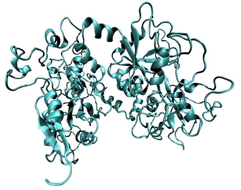
(a) LFG in its open state at $t=0$ ns.

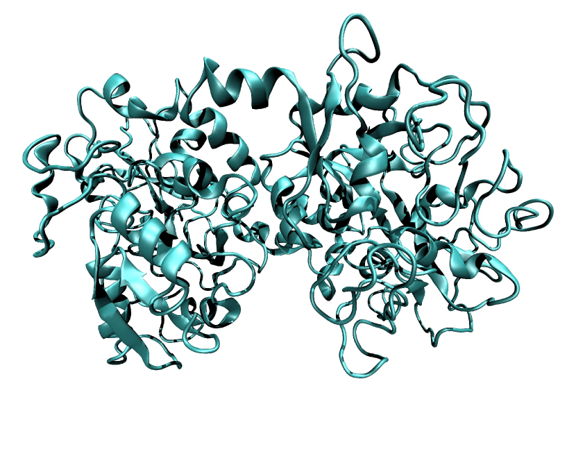
(b) LFG in its closed state at $t=19.6$ ns.

Figure 1: Snapshots of Lactoferrin protein in its open (a) and closed (b) states.

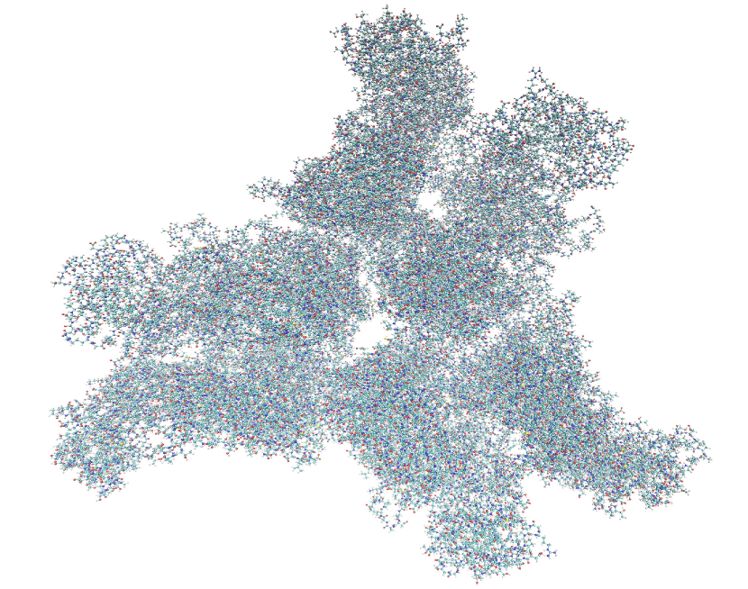
(a) N$\omega$v in its initial state at $t=0$ ns.

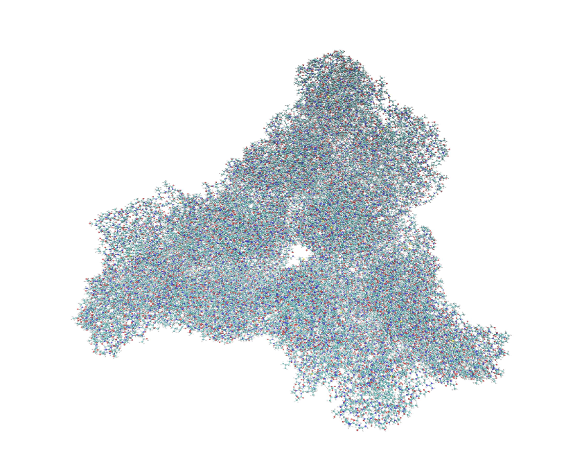
(b) N$\omega$v after shrinking at $t=3.0$ ns.

Figure 2: Snapshots of N$\omega$v triangular structure before (a) and after (b) contraction due to strong protein-protein interactions.

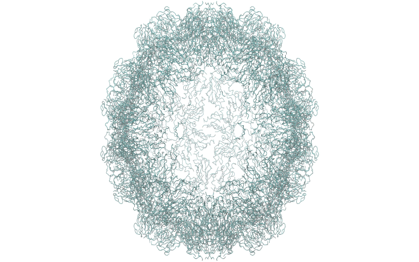
Figure 3: The full all-atom CCMV native capsid.

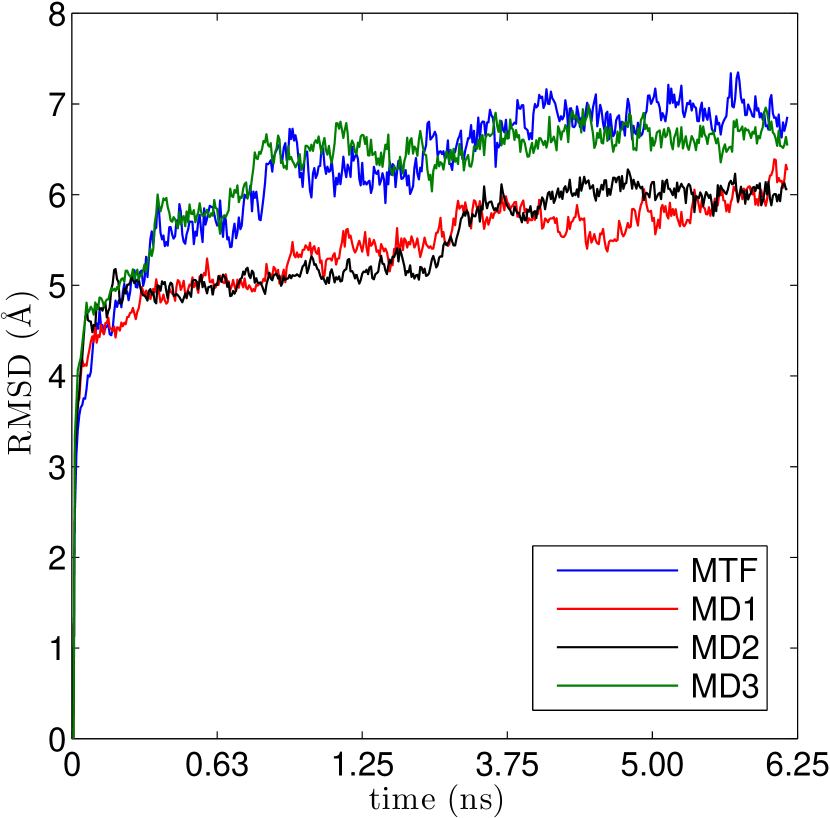
Figure 4: RMSD variation as a function of time for a series of three MD and one MTF runs.

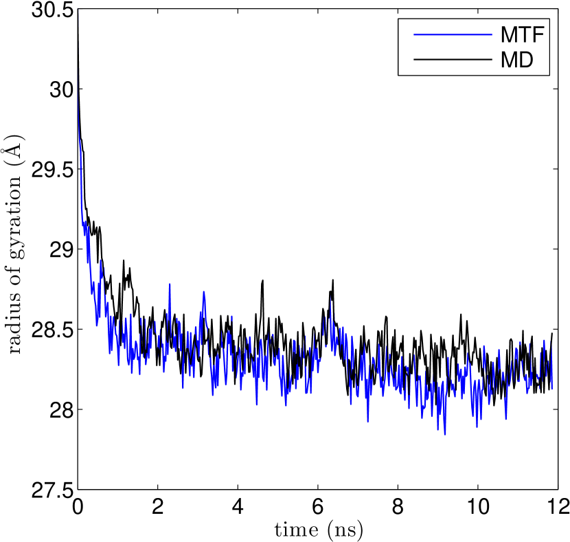
Figure 5: The radius of gyration decreases in time as Lactoferrin shrinks.

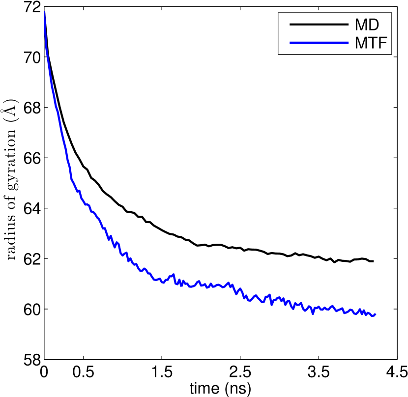
Figure 6: Temporal evolution of the radius of gyration of N$\omega$v computed using MD and MTF.

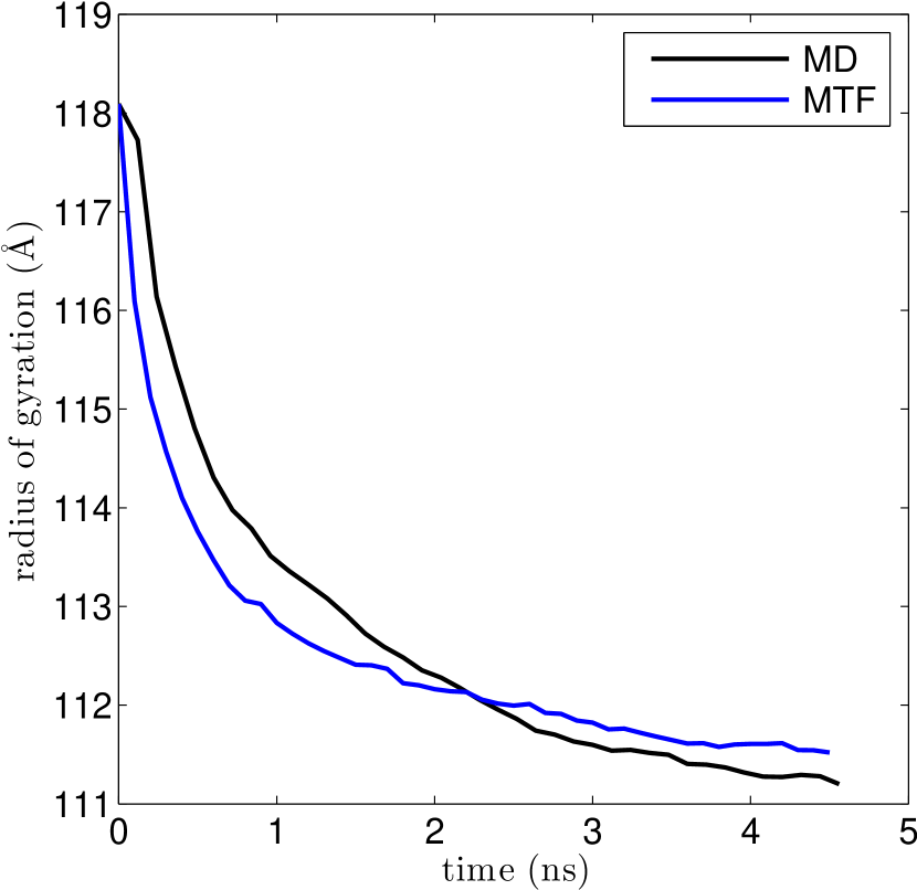
Figure 7: Temporal evolution of the radius of gyration of CCMV computed using MD and MTF.

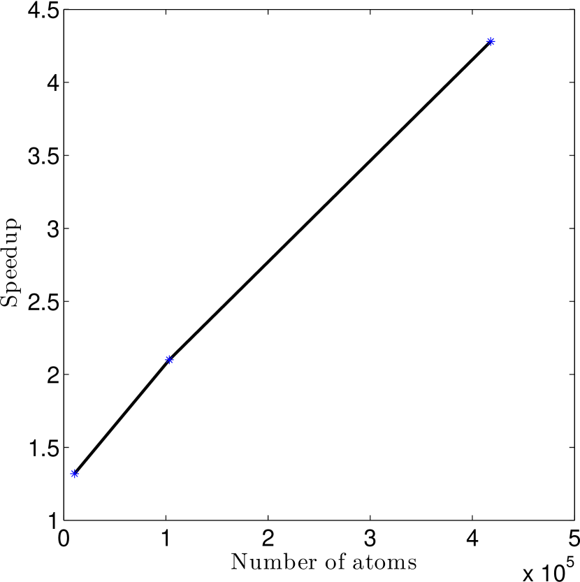
Figure 8: A plot of the speedup as a function of the system size shows the scalability of the MTF algorithm.

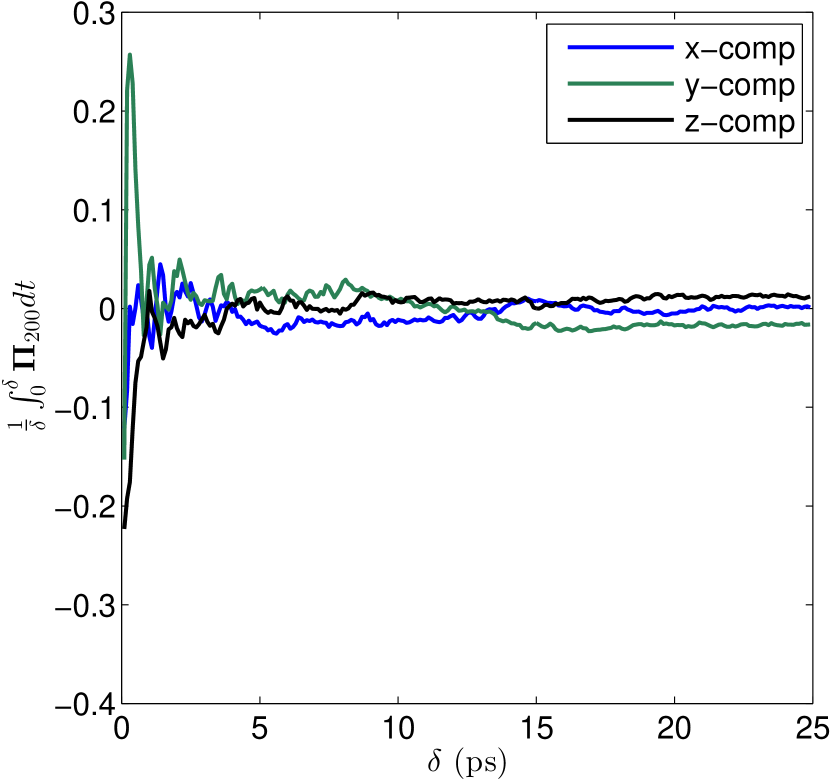
(a) A plot of the time integral of $\Pi$ for a high order CG $\Phi_{200}$.

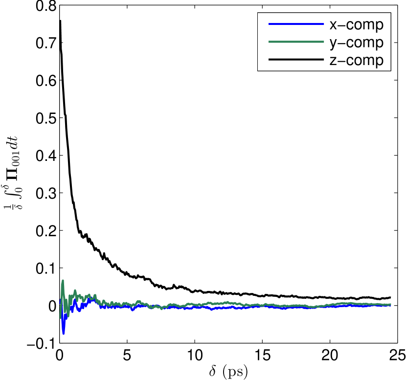
(b) A plot of the time integral of $\Pi$ for a low order CG $\Phi_{001}$.

Figure 9: Evidence for the validity of the stationarity hypothesis shown via the convergence of $\frac{1}{\delta}\int_{0}^{\delta}\Pi(t)dt$ as a function of $\delta$ for CG variables selected from among those used in simulating the contraction of N$\omega$v. Initially the integral experiences large fluctuations because with small $\delta$, only a relatively few configurations are included in the time average constituting the integral, but as $\delta$ increases, the statistics improves, and the integral becomes increasingly flat.

System	Size	Time	Speed-up
LFG	10,560	12.5 ns	1.32
N$\omega$V	103,317	4.30 ns	2.10
CWP	417,966	4.67 ns	4.28

Table 1: Speedup as a function of system size (number of atoms) for simulations run on 1x12, 4x12, and 8x12 cores for LFG, N$\omega$v, and CCMV, respectively.

Comparison between MD and MTF results are shown in 1. The dependence of speedup on the number of atoms in the system shown in 1 suggests that the benefit of MTF increases with the complexity of the system size (see Figure 8).

4 Conclusions

Mesoscopic systems express behaviors stemming from atom-atom interactions across many scales in space and time. Earlier approaches based on Langevin equations for coarse-grained variables did achieve efficiencies over MD without comprimising accuracy and captured key atomic scale details ^{33, 12}. However, such an approach requires the construction of diffusion factors, a task that consumes significant computational resources. This is because of the need to use large ensembles and construct correlation functions.

The multiscale factorization method used here introduces the benefits of multiscale theory of the LE. Here we revisit the Trotter factorization method within our earlier multiscale context. A key advantage is that the approach presented here avoids the need for the resource-consuming diffusion factors, and thermal average and random forces. The CG variables for the mesoscopic systems of interest do have a degree of stochastic behavior. In the present formulation, this stochasticity is accounted for via a series of MD steps used in the phase of the multiscale factorization algorithm wherein the $N-$atom probability density is evolved via $\mathcal{L}_{micro}$ , i.e. at constant value of the CG variables.

The MTF algorithm can be further optimized to produce greater speedup factors. In particular, the results obtained here can be significantly improved with the following: 1) after updating the CGs in the two-phase coevolution Trotter cycle, one must fine grain i.e. develop the atomistic configuration to be used as an input to MD. Recently, we have shown that the CPU time to achieve this fine graining can be dramatically reduced via a constraint method that eliminates bond length and angle strains, 2) information from earlier steps in discrete time evolution can be used to increase the time step and achieve greater numerical stability; while this was demonstrated for one multiscale algorithm ²⁹, it can also be adapted to the multiscale factorization method, and 3) the time stepping algorithm used in this work is the the analogue of the Euler method for differential equations, and greater numerical stability and efficiency could be achieved for a system of stiff differential equations using implicit and semi-implicit schemes ³⁴.

This project was supported in part by the National Science Foundation (Collaborative Research in Chemistry Program), National Institutes of Health (NIBIB), METAcyt through the Center of Cell and Virus Theory, Indiana University College of Arts and Sciences, and the Indiana University information technology services (UITS) for high performance computing resources.

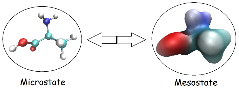
For table of contents use only.

References

- Phillips et al. 2005 Phillips, J. C.; Braun, R.; Wang, W.; Gumbart, J.; Tajkhorshid, E.; Villa, E.; Chipot, C.; Skeel, R. D.; Kale, L.; Schulten, K. J. Comput. Chem. 2005, 26, 1781–1802
- Spoel et al. 2005 Spoel, V. D.; Lindahl, E.; Hess, B.; Groenhof, G.; Mark, A. E.; Berendsen, H. J. C. J. Comput. Chem. 2005, 26, 1701–1718
- Cheluvaraja and Ortoleva 2010 Cheluvaraja, S.; Ortoleva, P. J. J. Chem. Phys. 2010, 132, 75102–75110
- Joshi et al. 2011 Joshi, H.; Singharoy, A.; Sereda, Y. V.; Cheluvaraja, S. C.; Ortoleva, P. J. Prog. Biophys. Mol. Biol. 2011, 107, 200–217
- Murtola et al. 2007 Murtola, T.; Falck, E.; Karttunen, M.; Vattulainen, I. J. Chem. Phys. 2007, 126, 75101–75114
- Reith et al. 2003 Reith, D.; Putz, M.; Muller-Plathe, F. J. Comput. Chem. 2003, 24, 1624–1636
- Bahar et al. 1997 Bahar, I.; Atilgan, R. A.; Erman, B. Folding and Design 1997, 2, 173–181
- Haliloglu et al. 1997 Haliloglu, T.; Bahar, I.; Erman, B. Phys. Rev. Letters 1997, 79, 3090–3093
- Shiha et al. 2006 Shiha, A. Y.; Arkhipov, A.; Freddolino, P. L.; Schulten, K. J. Phys. Chem. B 2006, 110, 3674–3684
- Shiha et al. 2007 Shiha, A. Y.; Freddolinoa, P. L.; Arkhipova, A.; Schulten, K. J. Struct. Biol. 2007, 157, 579–592
- Marrink et al. 2004 Marrink, S. J.; de Vries, A. H.; Mark, A. E. J. Phys. Chem. B 2004, 108, 750–760
- Singharoy et al. 2011 Singharoy, A.; Cheluvaraja, S.; Ortoleva, P. J. J. Chem. Phys. 2011, 134, 44104–44120
- Ortoleva 2005 Ortoleva, P. J. J. Phys. Chem. B 2005, 109, 21258–21266
- Pankavich et al. 2008 Pankavich, S.; Shreif, Z.; Ortoleva, P. J. Physica A 2008, 387, 4053–4069
- Pankavich et al. 2009 Pankavich, S.; Shreif, Z.; Miao, Y.; Ortoleva, P. J. J. Chem. Phys. 2009, 130, 194115–194124
- Abrams and Tuckerman 2008 Abrams, J. B.; Tuckerman, M. E. J. Phys. Chem. B 2008, 112, 15742–15757
- Noid et al. 2008 Noid, W. G.; Chu, J.-W.; Ayton, G. S.; Krishna, V.; Izvekov, S.; Voth, G. A.; Das, A.; Andersen, H. C. J. Chem. Phys. 2008, 128, 244114–244124
- Shea and Oppenheim 1996 Shea, J.-E.; Oppenheim, I. J. Phys. Chem. 1996, 100, 19035–19042
- Shea and Oppenheim 1997 Shea, J.-E.; Oppenheim, I. Physica A 1997, 247, 417–443
- Shea and Oppenheim 1998 Shea, J.-E.; Oppenheim, I. Physica A 1998, 250, 265–294
- Trotter 1959 Trotter, H. F. Proceedings of the American Mathematical Society 1959, 10, 545–551
- Hall 2003 Hall, B. C. Lie groups, Lie algebras, and representations: an elementary introduction; Springer, 2003; Vol. 10 (III); pp 36–37
- Tuckerman et al. 1992 Tuckerman, M.; Berne, B. J.; Martyna, G. J. J. Chem. Phys. 1992, 97, 1990–2001
- Miao and Ortoleva 2008 Miao, Y.; Ortoleva, P. J. Comput. Chem. 2008, 30, 423–437
- Miao et al. 2010 Miao, Y.; Johnson, J. E.; Ortoleva, P. J. J. Phys. Chem. B 2010, 114, 11181–11195
- Singharoy et al. 2012 Singharoy, A.; Joshi, H.; Miao, Y.; Ortoleva, P. J. J. Phys. Chem. B 2012, 116, 8423–8434
- Jaqaman and Ortoleva 2002 Jaqaman, K.; Ortoleva, P. J. J. Comput. Chem. 2002, 23, 484–491
- Pankavich et al. 2008 Pankavich, S.; Miao, Y.; Ortoleva, J.; Shreif, Z.; Ortoleva, P. J. J. Chem. Phys. 2008, 128, 234908–234921
- Singharoy et al. 2012 Singharoy, A.; Joshi, H.; Ortoleva, P. J. J. Chem. Inf. Model. 2012, 52, 2638–2686
- Romo and Grossfield 2009 Romo, T.; Grossfield, A. 31st Annual International Conference of the IEEE EMBS 2009, 2332–2335
- Norris et al. 1991 Norris, G. E.; Anderson, B. F.; Baker, E. N. Acta Crystallogr. Sect. B 1991, 47, 998–1004
- Taylor et al. 2003 Taylor, D. J.; Wang, Q.; Bothner, B.; Natarajan, P.; Finn, M. G.; Johnson, J. E. J. Chem. Commun. 2003, 22, 2770–2771
- Singharoy et al. 2012 Singharoy, A.; Sereda, Y.; Ortoleva, P. J. J. Chem. Theory Comput. 2012, 8, 1379–1392
- Iserles 2008 Iserles, A. A First Course in the Numerical Analysis of Differential Equations; Cambridge University Press, 2008; pp 53–63